

Abstract
Motivation: Many types of omics data are compiled as lists of connections between elements and visualized as networks or graphs where the nodes and edges correspond to the elements and the connections, respectively. However, these networks often appear as ‘hair-balls’—with a large number of extremely tangled edges—and cannot be visually interpreted.
Results: We present an interactive, multiscale navigation method for biological networks. Our approach can automatically and rapidly abstract any portion of a large network of interest to an immediately interpretable extent. The method is based on an ultrafast graph clustering technique that abstracts networks of about 100 000 nodes in a second by iteratively grouping densely connected portions and a biological-property-based clustering technique that takes advantage of biological information often provided for biological entities (e.g. Gene Ontology terms). It was confirmed to be effective by applying it to real yeast protein network data, and would greatly help modern biologists faced with large, complicated networks in a similar manner to how Web mapping services enable interactive multiscale navigation of geographical maps (e.g. Google Maps).
Availability: Java implementation of our method, named NaviCluster, is available at http://navicluster.cb.k.u-tokyo.ac.jp/.
Contact: thanet@cb.k.u-tokyo.ac.jp
Supplementary information: Supplementary data are available at Bioinformatics online.
1 INTRODUCTION
In the post-genomic era, a great number of biological data that are available via the Internet or obtained through high-throughput experiments are significantly inhibiting researchers from making sense of the data and communicating them to others in a concise and meaningful way (Evanko, 2010). Among these, one data type that has become increasingly common is binary relationship data, which are defined as sets of elements and 1-to-1 associations between them. Protein–protein interactions (PPI), correlatively expressed gene pairs, and genetic regulatory relationships exemplify this data type. They are conventionally presented using network (graph) visualization where nodes (vertices) and edges correspond to the elements and associations, respectively (Merico et al., 2009; Suderman and Hallett, 2007).
The network visualization is widely used because it is typically assumed to be more interpretable by humans than a long list of associations. High quality visualization should allow for effective investigation of the information, hypothesis generation and biological discovery (Merico et al., 2009). Unfortunately, network representations often fail to effectively convey information to readers in cases where the networks are large and complicated (e.g. >100 edges). The drawings of such networks, referred to as ‘hair balls’ (Suderman and Hallett, 2007), occur frequently when analyzing high-throughput biological data. To avoid being overwhelmed by such complicated networks, effective navigation approaches that can abstract data properly and present them insightfully at a right level of detail are hence required (Gehlenborg et al., 2010; Hu et al., 2007; O'Donoghue et al., 2010).
Hierarchical clustering is a technique used with many types of data, including networks or graphs, that meaningfully groups data elements in a recursive manner, thereby producing a hierarchy, or tree, of clusters (Andreopoulos et al., 2009) (Supplementary Figure S1). Higher levels in the hierarchy contain fewer, larger clusters, each of which encompasses more data elements (or nodes, in the case of networks) than lower levels. In the case of hair-balls, some methods (Abello et al., 2006; Freeman et al., 2007; Pavlopoulos et al., 2009; Royer et al., 2008; Vlasblom et al., 2006) use hierarchical clustering to create an interpretable visualization by displaying only the high-level clusters, thereby reducing the number of elements in the figure and abstracting the networks (e.g. the top panel in Supplementary Figure S1). By descending the hierarchy and showing the actual members of each cluster, detailed information can still be intuitively shown at a particular scale (e.g. the dotted arrows and regions in Supplementary Figure S1). A recent study reported that natural networks display hierarchical properties (Clauset et al., 2008), suggesting that hierarchical clustering of biological networks is both reasonable and promising.
Despite the advantages of hierarchical clustering, existing visualization methods using this technique have some drawbacks that hinder effective investigation of large biological datasets. First, some methods (Freeman et al., 2007; Shannon et al., 2003; Vlasblom et al., 2006) require researchers to provide information on hierarchies or clusters, data which is usually not known in advance. Secondly, existing methods do not allow for flexible navigation beyond fixed cluster boundaries (Abello et al., 2006; Freeman et al., 2007; Pavlopoulos et al., 2009; Royer et al., 2008; Vlasblom et al., 2006). In other words, they can visualize the members of one cluster at a time but do not support visualization and navigation of members of different clusters, despite the fact that nodes/clusters of interest to biologists may belong to various high-level nodes in the hierarchy (e.g. nodes in the light blue area in Supplementary Figure S1). Thirdly, existing methods are inappropriate for interactive, real-time navigation. Researchers frequently change their focus in the course of biological investigation to generate hypotheses and need to visualize different sets of nodes/clusters. Thus the long running times (minutes to hours) needed to produce the abstractions are unacceptable (Abello et al., 2006; Enright et al., 2002; Pavlopoulos et al., 2009; Royer et al., 2008). Methods that can provide appropriate abstractions of any given portion of the network rapidly and automatically, such as those that process about 100 000 nodes in seconds, are therefore necessary for efficient, interactive biological investigation. In addition to the previously mentioned problems, the clustering techniques employed by existing methods are often insufficient for abstracting large networks to a level that is simple enough for interpretation (Abello et al., 2006; Pavlopoulos et al., 2009; Royer et al., 2008). Recent investigations have revealed that in some common biological datasets, hub-like nodes tend to connect with low-degree nodes and the majority of nodes interact with only few partners (e.g. yeast PPI networks) (Yamada and Bork, 2009). Large, densely connected regions of such networks are therefore quite few; instead, small, densely connected modules are more frequently found. Consequently, even the highest level of the created hierarchies can contain over 100 clusters, resulting in cluttered and difficult to manage visualizations. Therefore, means for further abstraction are required to allow for effective navigation of large biological networks.
We developed an interactive, multiscale network navigation method with three advantages: (i) our method can work without a user-provided hierarchy; (ii) the method can rapidly, automatically and interactively produce abstractions of any region of the network, including nodes/clusters belonging to different ancestors in the hierarchy; and (iii) an intuitive visualization with a manageable amount of information is reliably produced at every step of navigation. The effectiveness of our method was confirmed using real yeast protein network data. Our approach will aid modern biologists faced with large and complicated network data.
2 METHODS
Our method consists of three components: an ultrafast graph clustering component, a property-based clustering component, and an interface that presents an abstracted view and permits researchers to flexibly choose nodes/clusters (Fig. 1). First, the method abstracts the whole network using the ultrafast graph clustering component. It detects topologically dense, connected regions, which may correspond to biologically meaningful clusters, such as protein complexes. It rapidly identifies clusters in huge networks of about 100 000 nodes within a few seconds, thus particularly suitable to be applied to the problem of interactive navigation of large and complicated networks. Additionally, if the property-based clustering needs to be executed afterwards, this graph clustering method displays another advantage in that it significantly reduces the number of clusters to be input to the next slower clustering.
Fig. 1.

A diagram of the presented method. For details, see the main text.
Secondly, in case the abstraction is insufficient because of the characteristics of the biological network, the property-based clustering component further abstracts the network to an extent sufficient for visual interpretation. This component automatically groups clusters with similar biological properties by utilizing the fact that biological entities are often assigned property information, such as Gene Ontology (GO) terms. The new clusters resulting from the property-based clustering are used in the next component instead of those generated by the ultrafast graph clustering component, thereby reducing the number of clusters on the screen. There are two main advantages of the property-based clustering: (i) the property-based clustering allows researchers to directly control the number of clusters shown on the screen through a parameter K of its underlying algorithm. To solve the problem of the cluttered visualization produced by applying only the graph clustering, the number of clusters shown on the screen must be decreased to an extent that biologists can manage to interpret. In addition, because the preferred numbers of clusters on the screen might differ according to the circumstances, it is important that biologists be allowed to adjust the number of clusters displayed; and (ii) because the clusters generated by the property-based clustering are based on the property information that carries biological meaning, the clusters are expected to be highly intuitive.
Thirdly, the resultant clusters/nodes are immediately displayed with meta-edges and property edges, which represent the numbers of edges that exist between any members of two clusters and the similarities between their properties, respectively. In the case that the number of clusters is less than the parameter K, the biggest cluster is recursively split until either the number of the clusters is equal to K or breaking only one more cluster makes the number of the clusters larger than K. While showing the abstracted view, the interface allows researchers to interactively zoom, move laterally beyond cluster boundaries, focus on an arbitrary set of clusters/nodes, etc. Any subset of the entire network of particular interest to the researcher can be fed into the clustering components and the abstracted view of that cluster is displayed. This cycle can be completed in a few seconds on a typical PC with a CPU of about 2 GHz and a memory of about 1 GB for datasets with 100 000 nodes, permitting truly interactive navigation of large biological networks.
2.1 Graph clustering
Graph clustering detects clusters in networks by finding densely connected sets of nodes where weighted connections of nodes within the sets are stronger/denser than weighted connections between nodes inside and outside of the set. This metric is called the modularity, or Q function (Newman and Girvan, 2004), and numerous graph clustering algorithms have been developed to identify clusters that optimize modularity (Blondel et al., 2008; Clauset et al., 2004; Newman and Girvan, 2004; Wakita and Tsurumi, 2007). The Newman–Girvan is a well-known, pioneering algorithm that iteratively removes edges most likely to lie between clusters, splitting the clusters into two, until no edges remain (Newman and Girvan, 2004). This process results in a dendrogram (a tree showing the order of the splits) and the best clustering can be identified from this tree by choosing the split with the highest modularity. This algorithm has a high computational cost, as it requires a traversal of all remaining edges at every step. Until recently, the best known algorithm developed to overcome this shortage with near-linear time complexity was devised by Wakita and Tsurumi (Wakita and Tsurumi, 2007). However, the speed of this algorithm was still insufficient and the quality of the clusters produced had room for improvement when incorporated into an interactive navigation of large networks (e.g. human gene networks of >20 000 nodes) (Blondel et al., 2008). Recently, Blondel et al. (2008) developed a breakthrough algorithm for quickly identifying high modularity clusters in huge networks of about 100 000 nodes (the Louvain algorithm). We found that this algorithm for finding meaningful communities in large and complicated networks could be applied to the problem of interactive navigation.
2.2 The Louvain algorithm
The Louvain algorithm works in two phases, as follows:
Starting from the state that each node belongs to a cluster different from every other node, for each node the algorithm considers its neighbors' clusters and moves the node to a neighboring cluster. The cluster to be joined is determined by choosing the movement that results in the highest positive modularity gain among all possible movements to the node's neighboring clusters. If no movements result in a positive gain in modularity, the node is not moved. This process is repeated until no members are added to/removed from any clusters and yields clusters with the maximum local modularity.
Every cluster from Phase 1 is then treated as a new node. For each pair of new nodes, an edge connecting them exists if there is at least one edge between any member of one of the new nodes and any member of the other. Edge weights are determined based on the number of previous edges. Self-loops are drawn on nodes to represent corresponding inter-cluster edges.
The output of Phase 2 is then fed back to Phase 1 and the algorithm iteratively runs these two phases until no additional changes are made. More details of this algorithm can be found in (Blondel et al., 2008).
This algorithm can finish clustering networks of 70 000 nodes in one second (Blondel et al., 2008). Thus, it works swiftly on many biological networks that generally contain less than 100 000 nodes (e.g. yeast or human PPI networks). The ultrafast speed of the algorithm is essential for accomplishing the goal of truly interactive navigation of large networks.
The clusters produced by this algorithm, which we call Louvain clusters or LCs, are characterized by high modularity. It has been shown that clusters with high modularity in biological networks correspond to biologically functional units [e.g. protein complexes in PPI networks and transcriptional modules in gene regulatory networks (Dunn et al., 2005)]. Thus, the LCs are expected to be intuitive and meaningful groups in navigation of biological networks.
Note that it is also possible to continue Louvain clustering to further reduce the number of clusters, even if the gain in modularity becomes negative. However, in such cases, the biological intuitiveness of the clusters produced would be lowered due to the decreased modularity (Dunn et al., 2005). Therefore, at this stage, it would be better to adopt another reliable source of information, in addition to the topology of the networks.
2.3 Property-based clustering
The property-based clustering component aims to decrease the complexity remaining after the application of the Louvain algorithm by further grouping LCs based on property information typically associated with the nodes (Supplementary Figure S2). The visualization step displays the clusters resulting from the property-based clustering instead of those generated by the graph clustering approach, thereby reducing the number of clusters on the screen. The VisANT tool works similarly to our property-based clustering and offers integrated visualization of the GO hierarchy and user-specified networks, but it requires the user to manually create clusters containing the same GO terms (Hu et al., 2009). In contrast, our property-based clustering automatically generates clusters having similar properties to achieve interactive navigation.
Let N be the number of nodes in the original input graph and L be the number of LCs. For each n, where 1 ≤ n ≤ N, node vn has a set of terms, T.(vn), that denotes the properties of the node (e.g. a set of GO terms). A weight, w(t), is given to each term t to quantify its importance (e.g. properties that are rare and/or of particular interest to researchers may be given higher weights). Let  and Tall = {tj | 1 ≤ j ≤ |Tall|}. For each LC, LCl, where 1 ≤ l ≤ L, let Prop(t, LCl) = | {v ∈ LCl|t ∈ T(v)}|/|LCl|. Then the property vector for LCl or PV (LCl) is a |Tall|-dimensional vector whose j-th element is the score of term tj, which is calculated as w(tj)Prop(tj, LCl). (Note that, in our implementation, a property term to be used for labeling LCl is the term th which is w(th)Prop(th, LCl) ≥ w(tj)Prop(tj, LCl), ∀j, 1 ≤ j ≤ |Tall|.) Next, the similarity between two LCs, LCa and LCb , is given as a normalized dot product of the two property vectors; that is, Sim(LCa, LCb) = PV(LCa)·PV(LCb)/PV(LCa)||PV (LCb)|. Then LCs having similar property vectors are grouped by the Farthest First Traversal K-center (FFT) algorithm (Andreopoulos et al., 2009). The FFT algorithm is a complexity-reducing variant of the K-means algorithm, where initial K cluster centers are chosen as follows. The first center (vector) is chosen randomly and each remaining center is determined by greedily choosing a vector farthest from the set of already chosen centers. The rest of the vectors are assigned to the cluster to which they are most similar.
3 IMPLEMENTATION
The proposed method was implemented as a Java 6 Swing application with a graphical interface for flexible navigation. The JUNG (Java Universal Network/Graph Framework) library (http://jung.sourceforge.net) was employed to create the visualization. Three input files are required to run the application: a node list file, an edge list file and a property information file. The node list file describes node names, property terms annotated with the nodes, and database names and IDs used in those databases (e.g. SGD for yeast proteins). The database information is used to provide URL links. The edge list file contains connected pairs of node names and the weights of the connections (weights describe how strongly the nodes are connected). The property information file describes the property terms in the node list file: terms' IDs, names, display names (used in labeling clusters in abstracted views), namespaces, default weights and their parent terms. In the case of the GO property information file bundled with the software, the default weights are terms' depths in the GO hierarchy. This treats more specific terms as more important properties. In addition, each term belongs to one of three namespaces (biological process, molecular function or cellular component). By using the namespace information, researchers can put heavier weights on all biological process terms at once if they want to group nodes having similar biological process terms, rather than other namespace terms. If parent terms are provided for each term, they are automatically assigned to the nodes that the term annotates as well. The is_a and part_of relationships in GO are handled by this entry. The implemented software, NaviCluster, works on any platform that can run Java 6. The program has a minimum memory requirement of 1 GB for networks of about 100 000 edges.
In addition to the highlighted features, NaviCluster has many additional functions designed for interactive network navigation. Views containing only nodes/clusters that the user wants to explore can be created, as well. Undo/Redo functions allow users to easily move backwards and forwards between previously created network views. As previously mentioned, users can adjust the namespace factors to change their importance, which changes the weights of all terms in the same namespaces, as long as at least one namespace weight is not zero. Furthermore, the number of clusters resulting from the property-based clustering, 12 by default, can be freely changed to match the individual preferences of the user. The user can trace a node of interest easily with the search function; the software can highlight the cluster in the current graph view that contains the node of interest. In addition, users can customize the view according to their preferences in many ways; for example, the property edges can be filtered based on the similarity value. Besides, visual appearances are designed to intuitively describe the different characteristics of the nodes/clusters and edges (e.g. node/cluster labels, cluster sizes and edge thicknesses). Context-specific popup menus, which contain links to external databases, are also available to accelerate knowledge discovery and hypothesis generation as much as possible.
4 RESULTS
4.1 Interactive and multiscale navigation
Our method provides zooming and re-centering functions, which imitate the functions of common Web mapping services such as Google Maps. The zooming function executes the two-stage clustering instantly, using all node members of the selected clusters as input, and displays the abstracted network afterwards. Given researcher-selected nodes/clusters, the re-centering function runs the clustering on all nodes in the entire network whose geodesic distances to the selected clusters/nodes are less than/equal to a provided value. The neighbor nodes do not need to be included in the current view; this function corresponds to the panning function Web mapping services provide to see surrounding regions. The resulting view shows the clusters/nodes of interest in the center of the display, as well as the nearby ‘neighbors’. By changing the geodesic distance value, both fine and rough visualization centered on the clusters/nodes of interest can be obtained. Note that the zooming operation can be run on more than one cluster at a time, useful for cases where the nodes of interest belong to different clusters. This function, as well as the re-centering function, correspond to seeing a map of several cities in different countries in Web mapping services and were not possible with previously existing methods.
4.2 Abstraction of large and complicated biological networks
Figure 2 illustrates the abstracted visualization of the entire Saccharomyces cerevisiae protein network YeastNet v.2 (Lee et al., 2007). The dataset contains 5483 yeast proteins (nodes) and 102 803 linkages (edges), and our implemented tool can generate this figure in just a few seconds on a typical PC. The log-likelihood scores indicating the probabilities of true functional linkages in YeastNet were adopted as the edge weights for the ultrafast graph clustering component. Edges with high weights connote that the protein pairs of the edges have strong relationships and thus highly likely to be grouped in the same clusters in the ultrafast graph clustering. GO terms assigned to the proteins in the SGD database [http://downloads.yeastgenome.org/ (access date: March 29, 2010)] were used as property information for the property-based clustering. The property-based clustering was configured to focus only on the biological process namespace because we wanted to group proteins involved in the same biological process. This can be done by excluding all terms of the other two namespaces in the property-based clustering—which can be easily performed using the namespace sliders in the implemented tool. The numbers displayed above clusters represent the numbers of nodes within the clusters and the labels following those numbers are the abbreviated property terms that can best describe the properties of the clusters, providing insight into the biological meaning of the clusters. Such property terms are the ones that are shared by most proteins in the clusters and meanwhile most specific (deepest in the GO hierarchy) among all terms annotated to the proteins in the clusters (see Section 2 for details). In case there are more than one cluster labeled with the same property term, the next highest score term of each cluster is additionally displayed in brackets to discriminate the cluster from the others. The display sizes of the clusters are proportional to linear normalizations of the numbers of the clusters over the interval from the minimum and the maximum numbers among all clusters. The color saturations of the clusters also reflect the number of proteins inside. Meta-edges are drawn between any two clusters that have at least one edge between at least one member in each of the two clusters (solid lines in Fig. 2). The gray number next to each meta-edge is the total numbers of all edges existing between the members of the two clusters, which are also reflected in the thickness of the meta-edge. In addition, a property edge is drawn between every pair of clusters if the similarity between their property vectors, represented by the associated gray number, is larger than a specified threshold (dashed lines in Fig. 3; the threshold is 0.1).
Fig. 2.
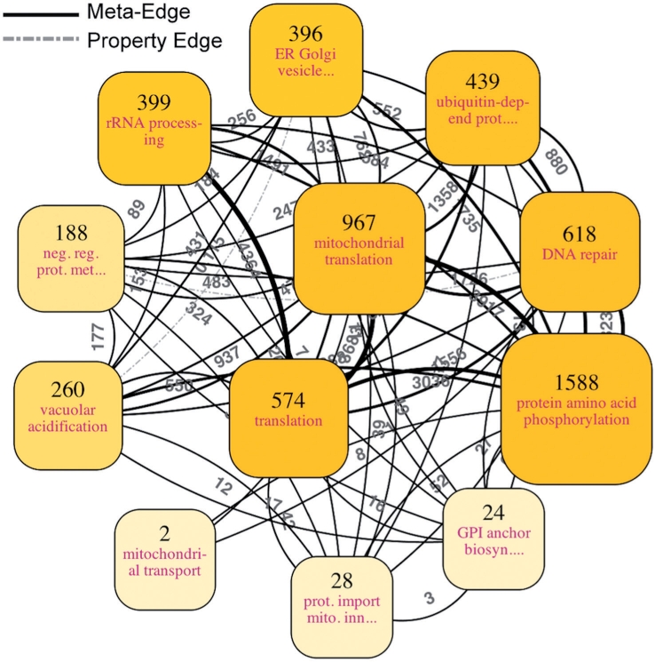
An abstracted view for all of YeastNet v.2, a probabilistic functional network containing 5483 yeast proteins and 102 803 linkages (Lee et al., 2007). The associated log-likelihood scores were adopted as edge weights and used in the ultrafast graph clustering. The implemented software, NaviCluster, directly produced the visualization with the number of clusters to be displayed set at 12. For detail, see the main text.
Fig. 3.

Multiscale navigation for a specific protein in a large network. This figure shows the hierarchical organization of the clusters encompassing Cla4, a protein of interest, which are highlighted in pink. The numbers by the arrows indicate the numbers of proteins contained in the processed sub-networks. Hexagons represent proteins that are not contained in any cluster. (A) The most abstract view (same as Fig. 2). Cla4 belonged to the highlighted protein amino acid phosphorylation cluster. After zooming in on this cluster, the clusters containing Cla4 of two deeper views were also the clusters labeled protein amino acid phosphorylation and were excluded for the sake of conciseness. (B) At this level, Cla4 was contained in the establishment of cell polarity cluster. Clusters labeled with the same property terms as those of others are discriminated by additionally displaying the next highest score terms in brackets. (C) Cla4 was contained in the regulation of exit from mitosis cluster. (D) The most specific view. Cla4 was clustered together with Ste20, Gic1, Gic2, Cdc24, Bem1, Skm1, Msb1, Msb2 and Tos2. A large version of this figure is available at Supplementary Figure 3.
4.3 Untangling hierarchical organization of large and complicated protein networks
Large biological networks can be interactively navigated in a multiscale manner as illustrated in Figure 3. Using the YeastNet v.2 dataset as an input network, Figure 3 demonstrates how the zooming and searching functions of our implemented tool can be employed together to lead researchers to the protein of interest, in this case Cla4. Cla4 is a p21-activated protein kinase that acts as an effector of Cdc42. It has been implicated in many important biological processes such as cell polarization (Bi et al., 2000; Bose et al., 2001; Gulli et al., 2000), cytokinesis (Benton et al., 1997; Cvrcková et al., 1995) and exit from mitosis (Bosl and Li, 2005; Höfken and Schiebel, 2004; Jensen et al., 2002; Seshan et al., 2002; Tiedje et al., 2008). In Figure 3, the clusters containing Cla4 are highlighted in all views; the granularities of detail in the views vary from coarsest to finest. Each zooming operation (a solid arrow) performs clustering on the member proteins of the highlighted cluster and immediately shows 12 more detailed clusters.
In the first view, which abstracts the whole network, the clusters are labeled with broad biological processes such as DNA repair, rRNA processing and translation (Fig. 3A). Cla4 is grouped under the protein amino acid phosphorylation cluster, which is highlighted. The members of this cluster are mostly involved in phosphorylation processes, that is also true for Cla4, which functions as a kinase to phosphorylate proteins. After zooming in on the protein amino acid phosphorylation cluster, one can find clusters of more specific processes, such as mitotic cell cycle spindle assembly checkpoint, pseudohyphal growth and establishment of cell polarity (Fig. 3B). In this view, Cla4 is found in the cluster involved in establishment of cell polarity, which is consistent with previous studies suggesting this role for the protein (Bi et al., 2000; Bose et al., 2001; Gulli et al., 2000). Some clusters found deeper in this cluster are characterized by actin filaments or budding processes (Fig. 3C); as expected, they are related to cell polarity. Cla4 is a member of the regulation of exit from mitosis cluster at this navigation level. After zooming in on this cluster, the final view illustrates the relationships between Cla4 and other proteins such as Gic1, Gic2 and Ste20 (Fig. 3D). In fact, these proteins were found to be involved in mitotic exit by three different mechanisms (Tiedje et al., 2008). Cla4 was discovered to promote mitotic exit and cytokinesis by activating a guanine nucleotide exchange factor, Lte1, which in turn causes the activation of Tem1, thereby terminating the M phase of the cell cycle (Jensen et al., 2002; Seshan et al., 2002; Tiedje et al., 2008). In addition, Gic1 and Gic2 were also proposed to be involved in stimulating mitotic exit in parallel with Cla4 by inhibiting GTPase-activating proteins of Tem1, both of which result in Tem1 activation (Höfken and Schiebel, 2004; Tiedje et al., 2008). Moreover, Cdc24 and Bem1, which play important roles upstream in the regulation of mitotic exit (Bi et al., 2000; Bose et al., 2001; Gulli et al., 2000; Tiedje et al., 2008), are also clustered together with Cla4 in this view.
This example illustrates that in all views proteins of related biological processes are clustered together sensibly and their roles are indicated informatively, correctly and appropriately based on the granularity of each view. The amount of information displayed is kept tractable by showing coarse and fine information on the abstracted and detailed views, respectively. Every zooming step is rendered in a matter of seconds, which allows researchers to gather interesting information at the desired degree of detail easily and effectively.
4.4 Discovering knowledge about proteins of interest from a large network intuitively and effectively
As zooming is always performed on all members of selected clusters, it alone is insufficient to provide flexible enough navigation for researchers to explore relationships between some nodes that may belong to different clusters. To fulfill this requirement, we designed the re-centering function. By performing re-centering, researchers can focus on nodes/clusters of interest and their relationships with other nodes within a specified geodesic distance from the entire network (i.e. not restricted to the nodes contained in the current view).
Figure 4A shows the view resulting from selecting the proteins Nas6, Rpn14, and Hsm3 and invoking the re-centering function to gather all direct interactors. Recent studies have reported that these three proteins, previously known to bind to regulatory particles of proteasomes, actually function as chaperones, assisting in the regulatory particle assembly in yeast (Funakoshi et al., 2009; Le Tallec et al., 2009; Roelofs et al., 2009; Saeki et al., 2009). In Figure 4A, the fundamental roles of the three proteins as proteasome-related proteins are delineated explicitly; specifically, they interact with many proteins involved in the ubiquitin-dependent protein catabolic process.
Fig. 4.
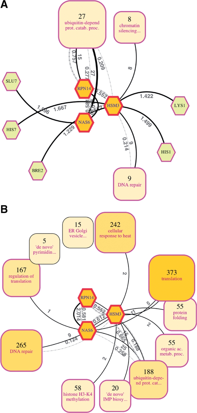
Re-centered views for retrieving knowledge from both direct and indirect neighbors of proteins of interest in a large network. Two views focusing on three proteins related to proteasome regulatory particle assembly (Nas6, Rpn14 and Hsm3) were created using the re-centering function. Edges not connected to these center proteins are omitted for clarity. (A) Re-centered with the geodesic distance from the central nodes set to one. Twenty seven of the 49 direct neighbors of the three proteins form a ubiquitin-dependent protein catabolic process cluster, nine form a DNA repair cluster and eight form a chromatin silencing at telomere cluster. (B) Re-centered with the geodesic distance set to two. This view delineates the more general functions of the proteins (see the main text). A large version of this figure is available at Supplementary Figure 4.
It is also possible to investigate the relationships between Nas6, Rpn14, and Hsm3 and other proteins that are farther from them, to understand their roles in a broader context (Fig. 4B; the abstracted view collecting all proteins within two hops from the three selected proteins). In addition to the relationship with the ubiquitin-dependent protein catabolic process cluster, this view reveals relationships with other clusters of more general processes. Among them, the relationships with the protein folding and cellular response to heat clusters actually suggest the recently reported roles of the three proteins as chaperones (proteins denatured due to heat are rescued by chaperones, which help fold and assemble proteins). It should be noted that these clusters were formed without using any property information from the three selected proteins.
These examples indicate that our method can be used to intuitively and effectively retrieve knowledge on nodes of interest from large and complicated networks. Abstraction of the three proteins' neighbors is necessary because, even if it is possible for biologists to manually investigate all 49 direct neighbors shown in Figure 4A, it is not practical to do the same for the 1443 indirect neighbors shown in Figure 4B. This is a fundamental issue because this indirect information suggested the chaperone role; however, it was not possible to interactively create these views using methods that depend on fixed cluster hierarchies.
5 DISCUSSION
To confirm the novelty and capabilities of the present method, we compared it to other existing visualization methods such as GenePro (Vlasblom et al., 2006), Power Graphs (Royer et al., 2008), VisANT (Hu et al., 2009), BioLayout Express3D (Freeman et al., 2007) and jClust (Pavlopoulos et al., 2009) (Supplementary Table 1). Our method was the only one capable of representing the hard-to-manage and complicated visualization of the overwhelming numbers of nodes and edges and providing the capability to navigate networks beyond cluster boundaries. GenePro, BioLayout Express3D and jClust can visualize clusters of nodes, but only at a single level. They do not support visualization of recursive clustering. VisANT provides multiscale visualization; however, the user must manually create metanodes (equivalent to clusters) themselves. CyOog (Power Graphs) hierarchically visualizes power nodes (equivalent to clusters) created by the Power Graph algorithm, but the speed is not fast enough to be used for interactive navigation of large biological networks.
It should be noted that our method is highly extendable in several ways. First, any type of property information, not just GO categories, can be used in the property-based clustering. For example, if a researcher is interested in diseases, she/he can use disease names associated with proteins derived from disease databases to investigate PPI networks by clustering proteins related to similar diseases. Secondly, because the clustering components of the present method can abstract any sub-network very rapidly, any interactive function for producing network views of interest can be achieved if modules for selecting appropriate clusters/nodes are implemented. For example, it is easy to devise a module that interactively produces networks of genes regulated by a selected regulatory factor, given information on gene regulatory relationships. Thirdly, the presented method is not limited to biological applications. In fact, it is general enough to be tailored to network data from other sources as well, as long as information adequately describing the properties of the nodes is provided. For example, citation networks of biomedical research articles can be explored with the MeSH (Medical Subject Headings) vocabularies that are stored in the MEDLINE database, and friendship networks of university students can be explored with information of class names they attend. In addition, implementing the method as a plug-in of an existing platform, e.g. Cytoscape (Shannon et al., 2003) would be a promising way to effectively integrate the benefits from the method with the abundant features of the platform, such as connection with important databases.
To summarize, we present the first method for interactive and multiscale navigation of large, complicated biological networks that displays appropriately abstracted views at all levels of detail. The specially designed interface, particularly the re-centering function, enables flexible navigation across cluster boundaries. Application to real biological network data demonstrates how it achieves the goal of providing effective, intuitive and interactive navigation, and why it is eminently suitable for large biological networks. As shown by analysis of Cla4, every time the researcher zooms in, clusters were constructed on the fly and visualized immediately along with meaningful labels. All views were informative as to the hierarchical structure of the network. As for Nas6, Rpn14 and Hsm3, their roles as chaperones were suggested in the view created by the re-centering function, which encompassed the indirect neighbors of these nodes. This outcome indicates that, in addition to the usual network exploration accomplished by displaying direct interactors, our methods can also uncover interesting hidden facts in large, complicated networks. This feature will help researchers formulate new hypotheses more easily and systematically, even if they possess little experience in bioinformatics. We believe that the presented method will aid modern biologists in discovering knowledge from massive binary-relationship datasets, which are accumulating at an accelerating pace.
Funding: Grant-in-Aid for Scientific Research on Priority Areas ‘Systems Genomics’ from the Ministry of Education, Culture, Sports, Science and Technology of Japan; Grant-in-Aid for Young Scientists (Start-up) from the Japan Society for the Promotion of Science. The funders had no role in study design, data collection and analysis, decision to publish or preparation of the manuscript.
Conflict of Interest: none declared.
Supplementary Material
REFERENCES
- Abello J., et al. ASK-GraphView: a large scale graph visualization system. IEEE Trans. Vis. Comput. Graph. 2006;12:669–676. doi: 10.1109/TVCG.2006.120. [DOI] [PubMed] [Google Scholar]
- Andreopoulos B., et al. A roadmap of clustering algorithms: finding a match for a biomedical application. Brief. Bioinform. 2009;10:297–314. doi: 10.1093/bib/bbn058. [DOI] [PubMed] [Google Scholar]
- Benton B., et al. Cla4p, a Saccharomyces cerevisiae Cdc42p-activated kinase involved in cytokinesis, is activated at mitosis. Mol. Cell Biol. 1997;17:5067–5076. doi: 10.1128/mcb.17.9.5067. [DOI] [PMC free article] [PubMed] [Google Scholar]
- Bi E., et al. Identification of novel, evolutionarily conserved Cdc42p-interacting proteins and of redundant pathways linking Cdc24p and Cdc42p to actin polarization in yeast. Mol. Biol. Cell. 2000;11:773–793. doi: 10.1091/mbc.11.2.773. [DOI] [PMC free article] [PubMed] [Google Scholar]
- Blondel V., et al. Fast unfolding of communities in large networks. J. Stat. Mech. 2008;2008:P10008. [Google Scholar]
- Bose I., et al. Assembly of scaffold-mediated complexes containing Cdc42p, the exchange factor Cdc24p, and the effector Cla4p required for cell cycle-regulated phosphorylation of Cdc24p. J. Biol. Chem. 2001;276:7176–7186. doi: 10.1074/jbc.M010546200. [DOI] [PubMed] [Google Scholar]
- Bosl W., Li R. Mitotic-exit control as an evolved complex system. Cell. 2005;121:325–333. doi: 10.1016/j.cell.2005.04.006. [DOI] [PubMed] [Google Scholar]
- Clauset A., et al. Hierarchical structure and the prediction of missing links in networks. Nature. 2008;453:98–101. doi: 10.1038/nature06830. [DOI] [PubMed] [Google Scholar]
- Clauset A., et al. Finding community structure in very large networks. Phys. Rev. E. 2004;70:066111. doi: 10.1103/PhysRevE.70.066111. [DOI] [PubMed] [Google Scholar]
- Cvrcková F., et al. Ste20-like protein kinases are required for normal localization of cell growth and for cytokinesis in budding yeast. Genes Dev. 1995;9:1817–1830. doi: 10.1101/gad.9.15.1817. [DOI] [PubMed] [Google Scholar]
- Dunn R., et al. The use of edge-betweenness clustering to investigate biological function in protein interaction networks. BMC Bioinformatics. 2005;6:39. doi: 10.1186/1471-2105-6-39. [DOI] [PMC free article] [PubMed] [Google Scholar]
- Enright A., et al. An efficient algorithm for large-scale detection of protein families. Nucleic Acids Res. 2002;30:1575–1584. doi: 10.1093/nar/30.7.1575. [DOI] [PMC free article] [PubMed] [Google Scholar]
- Evanko D. Supplement on visualizing biological data. Nat. Methods. 2010;7:S1. doi: 10.1038/nmeth0310-s1. [DOI] [PubMed] [Google Scholar]
- Freeman T.C., et al. Construction, visualisation, and clustering of transcription networks from microarray expression data. PLoS Comput. Biol. 2007;3:e206. doi: 10.1371/journal.pcbi.0030206. [DOI] [PMC free article] [PubMed] [Google Scholar]
- Funakoshi M., et al. Multiple assembly chaperones govern biogenesis of the proteasome regulatory particle base. Cell. 2009;137:887–899. doi: 10.1016/j.cell.2009.04.061. [DOI] [PMC free article] [PubMed] [Google Scholar]
- Gehlenborg N., et al. Visualization of omics data for systems biology. Nat. Methods. 2010;7:S56–S68. doi: 10.1038/nmeth.1436. [DOI] [PubMed] [Google Scholar]
- Gulli M., et al. Phosphorylation of the Cdc42 exchange factor Cdc24 by the PAK-like kinase Cla4 may regulate polarized growth in yeast. Mol. Cell. 2000;6:1155–1167. doi: 10.1016/s1097-2765(00)00113-1. [DOI] [PubMed] [Google Scholar]
- Höfken T., Schiebel E. Novel regulation of mitotic exit by the Cdc42 effectors Gic1 and Gic2. J. Cell. Biol. 2004;164:219–231. doi: 10.1083/jcb.200309080. [DOI] [PMC free article] [PubMed] [Google Scholar]
- Hu Z.J., et al. VisANT 3.5: multi-scale network visualization, analysis and inference based on the gene ontology. Nucleic Acids Res. 2009;37:W115–W121. doi: 10.1093/nar/gkp406. [DOI] [PMC free article] [PubMed] [Google Scholar]
- Hu Z.J., et al. Towards zoomable multidimensional maps of the cell. Nat. Biotechnol. 2007;25:547–554. doi: 10.1038/nbt1304. [DOI] [PubMed] [Google Scholar]
- Jensen S., et al. Spatial regulation of the guanine nucleotide exchange factor Lte1 in Saccharomyces cerevisiae. J. Cell. Sci. 2002;115:4977–4991. doi: 10.1242/jcs.00189. [DOI] [PubMed] [Google Scholar]
- Le Tallec B., et al. Hsm3/S5b participates in the assembly pathway of the 19S regulatory particle of the proteasome. Mol. Cell. 2009;33:389–399. doi: 10.1016/j.molcel.2009.01.010. [DOI] [PubMed] [Google Scholar]
- Lee I., et al. An improved, bias-reduced probabilistic functional gene network of baker's yeast Saccharomyces cerevisiae. PLoS ONE. 2007;2:e988. doi: 10.1371/journal.pone.0000988. [DOI] [PMC free article] [PubMed] [Google Scholar]
- Merico D., et al. How to visually interpret biological data using networks. Nat. Biotechnol. 2009;27:921–924. doi: 10.1038/nbt.1567. [DOI] [PMC free article] [PubMed] [Google Scholar]
- Newman M.E.J., Girvan M. Finding and evaluating community structure in networks. Phys. Rev. E. 2004;69:026113. doi: 10.1103/PhysRevE.69.026113. [DOI] [PubMed] [Google Scholar]
- O'Donoghue S., et al. Visualizing biological data-now and in the future. Nat. Methods. 2010;7:S2–S4. doi: 10.1038/nmeth.f.301. [DOI] [PubMed] [Google Scholar]
- Pavlopoulos G.A., et al. jClust: a clustering and visualization toolbox. Bioinformatics. 2009;25:1994–1996. doi: 10.1093/bioinformatics/btp330. [DOI] [PMC free article] [PubMed] [Google Scholar]
- Roelofs J., et al. Chaperone-mediated pathway of proteasome regulatory particle assembly. Nature. 2009;459:861–865. doi: 10.1038/nature08063. [DOI] [PMC free article] [PubMed] [Google Scholar]
- Royer L., et al. Unraveling protein networks with power graph analysis. PLoS Comput. Biol. 2008;4:e1000108. doi: 10.1371/journal.pcbi.1000108. [DOI] [PMC free article] [PubMed] [Google Scholar]
- Saeki Y., et al. Multiple proteasome-interacting proteins assist the assembly of the yeast 19S regulatory particle. Cell. 2009;137:900–913. doi: 10.1016/j.cell.2009.05.005. [DOI] [PubMed] [Google Scholar]
- Seshan A., et al. Control of Lte1 localization by cell polarity determinants and Cdc14. Curr. Biol. 2002;12:2098–2110. doi: 10.1016/s0960-9822(02)01388-x. [DOI] [PubMed] [Google Scholar]
- Shannon P., et al. Cytoscape: a software environment for integrated models of biomolecular interaction networks. Genome Res. 2003;13:2498–2504. doi: 10.1101/gr.1239303. [DOI] [PMC free article] [PubMed] [Google Scholar]
- Suderman M., Hallett M. Tools for visually exploring biological networks. Bioinformatics. 2007;23:2651–2659. doi: 10.1093/bioinformatics/btm401. [DOI] [PubMed] [Google Scholar]
- Tiedje C., et al. The Rho GDI Rdi1 regulates Rho GTPases by distinct mechanisms. Mol. Biol. Cell. 2008;19:2885–2896. doi: 10.1091/mbc.E07-11-1152. [DOI] [PMC free article] [PubMed] [Google Scholar]
- Vlasblom J., et al. GenePro: a Cytoscape plug-in for advanced visualization and analysis of interaction networks. Bioinformatics. 2006;22:2178–2179. doi: 10.1093/bioinformatics/btl356. [DOI] [PubMed] [Google Scholar]
- Wakita K., Tsurumi T. Finding community structure in mega-scale social networks. ArXiv Comp Sci. 2007:0702048. e-prints. [Google Scholar]
- Yamada T., Bork P. Evolution of biomolecular networks: lessons from metabolic and protein interactions. Nat. Rev. Mol. Cell. Biol. 2009;10:791–803. doi: 10.1038/nrm2787. [DOI] [PubMed] [Google Scholar]
Associated Data
This section collects any data citations, data availability statements, or supplementary materials included in this article.