Persistence of Past Stimulations: Storing Sounds within the Inner Ear

Abstract

Tones cause vibrations within the hearing organ. Conventionally, these vibrations are thought to reflect the input and therefore end with the stimulus. However, previous recordings of otoacoustic emissions and cochlear microphonic potentials suggest that the organ of Corti does continue to move after the end of a tone. These after-vibrations are characterized here through recordings of basilar membrane motion and hair cell extracellular receptor potentials in living anesthetized guinea pigs. We show that after-vibrations depend on the level and frequency of the stimulus, as well as on the sensitivity of the ear. Even a minor loss of hearing sensitivity caused a sharp reduction in after-vibration amplitude and duration. Mathematical models suggest that after-vibrations are driven by energy added into organ of Corti motion after the end of an acoustic stimulus. The possible importance of after-vibrations for psychophysical phenomena such as forward masking and gap detection are discussed.

Introduction

The hearing organ is composed of sensory cells and supporting cells, all resting on the basilar membrane (BM). Sound-evoked BM vibration will be sensed by the outer hair cells, which respond by producing force (e.g., 1–4). Such forces increase hearing sensitivity and frequency selectivity through a nonlinear feedback process that remains poorly characterized. Most models of hearing organ function assume that these forces amplify sound-evoked motions on a cycle-by-cycle basis by feeding energy into the traveling wave that propagates within the hearing organ; see Patuzzi (5).

Although force production is generally thought to occur on a cycle-by-cycle basis, its onset and offset kinetics remains the subject of speculation. Because force production is initiated by the acoustic stimulus, it may be assumed to end when the stimulus is removed. However, some recordings of BM motion show that high-level tones can produce vibrations that continue after the end of the stimulus (6), and similar after-effects are also evident in cochlear microphonic potentials (7,8) and in recordings of otoacoustic emissions (9). The source of these effects is unknown.

In this article, we show that after-vibrations are present at moderate stimulus levels and gradually become more prominent as the stimulus level increases. These after-vibrations appear to be driven by sustained force production within the inner ear—a form of short-term memory of past stimulations.

Methods

Animal preparation

Young pigmented guinea pigs weighing 250–450 g were used in this study. The Animal Care and Use Committee at Oregon Health & Science University approved all animal procedures. Animals were anesthetized with ketamine (40 mg/kg) and xylazine (10 mg/kg) and prepared for recording of BM velocities as previously described (10,11).

All animals were tracheotomized, but artificial ventilation was not used. The temperature of the animal was maintained at 38°C using a heating blanket controlled by a rectal probe. The middle ear muscles were transected and the BM exposed after widely opening the bulla. To increase the reflectance to a level useable for interferometric motion recordings, a few gold-coated glass beads were placed on the BM. To minimize surgically induced hearing loss, cochlear performance was continuously monitored using the simple difference tone distortion product, which was recorded by an electrode in the round window niche (12). Whenever the amplitude decreased, surgery was temporarily halted to allow recovery. The round window electrode was also used for recording auditory nerve compound action potential audiograms. This report is based on three exceptionally sensitive animals, two of which had no measureable loss of compound action potential thresholds as a result of surgery.

Laser velocimetry, sound stimulation, and data acquisition

BM motion was measured by focusing the light from a laser velocimeter (OFV 1102, Polytec, Waldbronn, Germany) on the reflecting bead mentioned previously.

All sound stimuli were delivered to the ear through a custom speculum fitted tightly into the ear canal to form a closed sound field. A sensitive microphone measured sound pressures near the tympanic membrane. Stimuli were generated with a digital-to-analog converter (System II, Tucker-Davis Technologies, Alachua, FL) and sampled with the System II analog-to-digital converter. Digital attenuators were used to set the stimulus level. The tones had either 1- or 2-ms onset and offset time with the shape of a Hanning window. The use of tone burst (rather than an impulse) allows separating and comparing the onset versus steady state versus offset kinetics, application of a single stimulus frequency, and exploring the role of nonlinearity. All records shown are averages of 100–1000 stimulus presentations. More averaging was used at the lower stimulus levels. Electrical and mechanical data were acquired with an identical number of averages. Tuning curves were acquired with a lock-in amplifier (SR830, Stanford Research Systems, Sunnyvale, CA), using a time constant of either 100 or 500 ms, depending on the stimulus level.

Electrophysiology

Local electrical potentials in the organ of Corti were measured after completing motion recordings. A motorized manipulator was used to advance microelectrodes toward the hearing organ through the opening used for vibration measurements. Under visual control, the tip of the electrode was positioned near the tunnel of Corti. Penetration of cells on the BM was evident by a transition to a negative direct current potential (usually near −70 mV). As the electrode was advanced further, this negative potential vanished; the amplitude of the cochlear microphonics increased substantially as the tip entered the fluid spaces near the cell bodies of the outer hair cells.

Electrodes pulled from borosilicate glass capillaries had tip diameters around 1 μm, and impedances in the range of 1–10 MΩ when filled with 3 M KCl solution. These relatively large electrodes were used to minimize filtering of the recorded potentials by the resistance and capacitance of the electrode.

Recordings were performed with a BMA-200 amplifier (CWA, Ardmore, PA) connected to the lock-in amplifier or the System II hardware mentioned previously. The frequency response of each electrode was calibrated while still in position within the organ of Corti, using the procedure described by Baden-Kristensen and Weiss (13, see also 11). These calibrations showed that electrodes behaved as single-pole low-pass filters with cutoff frequencies in the range 1–5 kHz. The high-frequency phase response of the electrode deviated from those expected from a single-pole filter. However, this discrepancy has little practical importance, because all the data were corrected for the filtering effects using the measured frequency response of the electrode rather than the fitted curves.

Following measurements of organ of Corti potentials, BM velocities were again measured, using identical stimulus parameters. Because electrode penetration frequently induced some loss of auditory sensitivity, all comparisons reported in this article use BM data acquired after the electrode penetration.

Signal processing

To reduce noise and remove small direct current offsets, all data were filtered offline using a phaseless second-order filter with passband from 4 to 40 kHz. The short-time Fourier transform was used to evaluate changes in response amplitudes over time, and the Hilbert transform for assessing changes in instantaneous phase and frequency. The Hilbert transform was computed with an algorithm based on the fast Fourier transform. Central differences were used to obtain the instantaneous frequency. Further details of these computations are given in the Results section where pertinent. To find peaks in the time waveforms, downward zero-crossings of the first derivative that exceeded a predetermined threshold slope were found. Additionally, the peaks had to exceed a preset amplitude threshold. All peaks were verified by visual inspection of the time waveforms. Computations were performed using MATLAB (The MathWorks, Natick, MA).

Results

After-vibrations on the BM

In good preparations, the BM continues to vibrate following the end of a pure-tone stimulus. Fig. 1 A shows the BM response to a characteristic frequency (CF) stimulus at 104 dB SPL in a sensitive ear with little loss in compound action potential thresholds at the time of recording. Although the stimulus declined smoothly, ending close to 8 ms, the BM response shows a sudden increase in amplitude near 10 ms that is followed by a gradual cessation of vibration. Several hours later, a substantial loss of auditory sensitivity had occurred. This led to a slight increase in BM vibrations during the stimulus (Fig. 1 B) and a complete loss of after-vibrations, as seen more clearly in Fig. 1, C and D, which shows the 10–30-ms time window at an expanded scale. A detailed examination of the data in panel C shows that low-level periodic motion at the stimulus frequency was present as late as 25 ms. No such motion was observed in the insensitive ear (D).

Figure 1.

After-vibrations are seen only in preparations with pristine sensitivity. The record shown in panel A was acquired from a sensitive animal. Data in panel B was recorded several hours later, when the preparation had suffered a substantial loss of auditory sensitivity. Panels C and D show the same data as in A and B at an expanded scale. The CF was 19 kHz and the stimulus level 104 dB SPL. Responses are averages of 100 stimulus presentations.

After-vibrations are examined in more detail in Fig. 2, using data from a different preparation. Note that the onset of the stimulus is associated with an overshoot in the BM velocity, which is absent from the stimulus, and that vibrations continue after the end of the stimulus. Close examination reveals that stapes motion ends at 8.4 ms, as seen in the inset in panel B. In contrast, the BM shows a complex vibration pattern with prominent amplitude modulations (inset in Fig. 2 A) that continue until the end of the recording window (at 30 ms). The amplitude spectrum (Fig. 2 C) shows that these vibrations are not noise. Note the single, narrow peak centered on the frequency of the stimulus that preceded these vibrations, 19.2 kHz. The velocity magnitude is ∼11 μm/s, more than 10 dB above the noise floor of the recording. Although this magnitude is low, tuning curves showed similar vibration amplitude in response to CF tones at around 20 dB SPL. The average magnitude of after-vibrations in the 20-ms time window after stopping the stimulus was 9 ± 2 μm/s (mean ± standard error, n = 3, 19.2 kHz, and 104 dB SPL, all three preparations had best frequencies near 19 kHz and were highly sensitive as judged from compound action potential audiograms).

Figure 2.

Offset effects in guinea pig BM motion. Responses at 84 and 104 dB SPL are the averages of 100 stimulus presentations, while 1000 averages were used at lower levels. (A) BM velocity response to a 6-ms tone burst at the best frequency of the recording location, 19.2 kHz. Stimulus level 104 dB SPL. The inset shows the part of the record between 10 and 30 ms. Scale bars in the inset equal 4 ms and 40 μm/s. (B) The input waveform as reflected in the motion of the stapes. The inset is a magnified version with scaling identical to the inset in A. (C) Frequency spectrum of the last 20 ms of the recording. (D) Instantaneous frequency at 84 and 104 dB SPL in a different preparation. Note that the local frequency is nearly constant except for the rapid rise at the onset of the tone. (E) Spectrogram of BM and stapes motion at 19.2 kHz and 103 dB SPL. A 10-cycle window was advanced one sample at a time through the record. Close to identical results were obtained by calculating the envelope using the absolute magnitude of the Hilbert transform. (F). Spectrogram computed with parameters identical to panel E. Stimulus level 43 dB SPL. Note that the stapes velocity could only be recorded in response to intense stimuli, and the stapes response displayed here is the same as in panel E. This simplification is justified because stapes vibrations scale linearly with intensity.

To further characterize the after-vibration, the Hilbert transform was used to compute its instantaneous frequency. This revealed that the beginning of the BM vibration was associated with a frequency glide that developed in only a few hundred microseconds (Fig. 2 D, average starting frequency 16 ± 2.5 kHz). The glide remained the same when increasing the stimulus level from 84 to 104 dB SPL. During the acoustic stimulus, the instantaneous frequency was constant and equal to the stimulus frequency; slight oscillations are seen during stimulus offset, but the local frequency settles on the stimulus frequency after a few milliseconds. These data show that the early part of the after-vibrations have a single well-defined frequency. Although minor oscillations do occur, these are smaller than the changes seen during stimulus onset. Instantaneous frequency calculations rely on taking the derivative of the phase that makes them sensitive to noise. Beyond 14 ms, the local frequency could not be reliably calculated, although periodic vibrations with a spectrum like the one displayed in Fig. 2 C were present until the end of the recording window at 30 ms.

Because the after-vibrations have nearly constant frequency, their magnitude variation can be examined at high time resolution with the short-time Fourier transform. The magnitude at the stimulus frequency is displayed in Fig. 2 E together with the similarly computed stapes vibrations (integration time 500 μs). Note the short delay between the onsets of stapes motion and BM vibration (∼100 μs). The two signals begin almost contemporaneously, but behave very differently after the end of the stimulus. Stapes vibrations quickly approach the noise floor, reflecting the 1-ms offset time of the stimulus, but BM vibrations decay slowly. The noise floor is reached transiently near 15 ms and again near 20 ms, but vibrations remain ∼6 dB above the noise floor at the end of the recording window. These after-vibrations occur in the absence of external acoustic stimulation, a fact that was verified by recording sound pressures in the ear canal with a sensitive microphone.

These effects are not restricted to high stimulus levels. The response to a 43-dB SPL stimulus is shown in Fig. 2 F. Here, an ∼370 μs delay between the onset of stapes motion and the first detectable movement of the BM is evident. In addition, the overshoot near the beginning, which was prominent at 104 dB SPL, is absent. At the offset, note that the stapes movement declines quickly, whereas the BM shows a gradual decay that results in a 940 μs horizontal gap between the two curves.

To further characterize after-vibrations, a peak-detection algorithm was used to estimate the number of excess cycles in BM movements as compared to the stapes. Evidently, the extent of after-vibration depends on both stimulus level and frequency (Fig. 3 A). The largest number of extra cycles (156 ± 29) is seen after high-level stimulations near the best frequency of the recording location, 19.2 kHz, but excess cycles are present at every stimulus level. We note that the original stimulus contained 154 cycles, therefore the after-vibrations equate to a doubling of the response duration on average. The number of excess peaks is reduced when the stimulus moves to 16.7 kHz (91 ± 16). At 14.7 kHz, the most intense stimulus triggers a slight after response (26 ± 8 cycles), but at low levels, stapes vibrations are more numerous. This is a trivial result of the low sensitivity of the recording location for sounds at this frequency. The beginning and end of the 14.7 kHz-stimulus is simply too weak to result in measurable BM vibration. The number of extra cycles was not affected by an increase of the rise and fall time from 1 to 2 ms, although the pattern of peaks and dips in the amplitude shifted, as detailed below.

Figure 3.

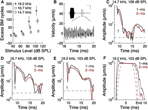
Frequency and level dependence of after-vibrations. (A) Excess cycles on the BM as a function of stimulus frequency and level. Error bars denote ±1 SE. Note that the shorter period time at higher frequencies will result in a larger number of excess cycles for a given duration of the memory vibration. However, this effect explains only a small part of the apparent difference between the three frequencies. (B) Response to a 108-dB SPL stimulus at 14.7 kHz. The graph shows a magnified version of the boxed area in the inset. In this inset, the vertical scale bar indicates 10 mm/s and the horizontal scale bar 5 ms. (C) Amplitude at the stimulus frequency as a function of time. Integration time 10 cycles. The response to tones with a 1- and 2-ms rise and fall time is displayed. (D) BM response at 16.7 kHz at two different rise times. (E) BM response at the CF. (F) Distortion of the response envelope. The scaled envelopes of the stimuli are shown by dashed lines, and that of the BM response by solid lines.

For the 14.7-kHz stimulus, the waveform of the BM vibration was close to a mirror of the input, as seen in the inset in Fig. 3 B. At first sight, this response looks minimally interesting. However, close examination of the 30-ms recording window revealed that periodic vibrations occur between 15 and 20 ms. Although there are substantial amplitude variations (Fig. 3 B), Fourier transformation of data within this time window resulted in a single narrow peak centered at the stimulus frequency, with magnitude ∼10 μm/s. Thus, even though the stimulus was far removed from the low-level CF of the recording location, long-delay components are present. This long-delay component is shown in more detail in Fig. 3 C. Although the after-vibration decays to the noise floor at around 11 ms, it rises again ∼5 ms later. The surprise here is that after-vibrations always occur at the stimulus frequency and show no tendency of transitioning toward the CF of the recording location, which is much higher.

Although the total number of excess cycles was unaffected by the rise and fall time of the stimulus, Fig. 3 C shows that the shape of the envelope is altered, an effect noted in all preparations showing substantial after-vibrations. At a rise/fall time of 1 ms (black line in Fig. 3 C), there is a dip in the amplitude near 9 ms (vertical arrow), which is immediately followed by a peak. A doubling of the rise time abolished both the dip and the ensuing peak and instead, a smooth decline in amplitude is seen (gray line, red online). Furthermore, the long-delay component near 15 ms occurred slightly earlier for the 2-ms rise time. A similar shift in the valleys is seen at 16.7 kHz (Fig. 3 D), where the 9-ms dip and following peak are absent when the fall time of the stimulus increases (vertical arrow). At 19.2 kHz, the dip and peak shift to the left when the rise time increases (Fig. 3 E). There was also pronounced distortion during the rising and falling phase, and this distortion was influenced by the rise and fall time. In Fig. 3 F, the shape of the tone bursts is given by the dashed gray line (red online) and black lines and the measured responses by the solid lines. For both rise times, the response of the BM grows much faster than the stimulus, and in both cases there is an overshoot before the response settles. Note that the shape of the 2-ms response is almost identical to the 1-ms stimulus, and the rising phase of the 1-ms stimulus is not visible in this figure. The tick mark labeled End is at the last detectable stapes oscillation. Now, the 1-ms and 2-ms response has almost the same amplitude. The difference between the stimulus envelope and the response envelope is now larger at 2 ms , and the envelope distortion could therefore be said to be more severe for the 2-ms fall time, a clearly nonlinear effect.

We also examined the effect of increased stimulus duration, but the length of the stimulus did not appear to significantly influence after-vibrations.

BM motion and organ of Corti potentials

To probe the mechanisms underlying after-vibrations, we recorded electrical potentials within the tunnel of Corti. Because of the limited space constant of this compartment, these potentials originate from a small group of hair cells surrounding the electrode (14,11). Electrical and mechanical tuning curves are generally very similar, but tuning is less sharp for the organ of Corti potentials and the peak is at a different frequency (Fig. 4). Previous studies suggest that these differences are due to interactions among potentials generated by neighboring hair cells vibrating at different phases (11).

Figure 4.

Tuning of organ of Corti potentials (gray lines, right scale) and BM velocity (black line, left scale). Stimulus levels 55 and 70 dB SPL.

The phase relations between the organ of Corti potential and the BM motion were stereotypical during the driven part of the response, as illustrated in Fig. 5, A and B. Note that electric potentials have a phase lead at the onset (Fig. 5 A) that was maintained during the steady-state part of the response (Fig. 5 B). Fourier transformation of the data during the steady-state part revealed that the relative phase of the two signals depended on the stimulus level for tones near the CF. At 43 dB SPL, the average phase lead for the organ of Corti potential was 84° ± 24°; this lead decreased to 46° ± 23° at levels >100 dB SPL. At frequencies much below CF, no level-dependent phase changes were observed.

Figure 5.

Phase relations among the BM velocity and organ of Corti potentials. (A) From its onset, electrical potentials lead the BM velocity. This lead is maintained during the steady-state part of the signal (B), but changes during the offset (C). Stimulus frequency 16.7 kHz, 104 dB SPL. All data are compensated for electrode and interferometer amplitude and phase response. Data from a different preparation (D) shows a consistent change in the relative phase of the two signals. Stimulus levels ranged from 43 to 103 dB SPL at the CF (19.2 kHz), using a rise/fall time of 1 ms at 43 and 63 dB SPL and 2 ms at 83 and 103 dB SPL.

The offset of the response was considerably more complicated (Fig. 5 C). Near 8.2 ms, the organ of Corti potential was close to antiphasic to the BM motion (left vertical arrow in Fig. 5 C), but rapid phase modulation was seen thereafter and at 8.5 ms, the two signals are in-phase (right vertical arrow). These phase changes were quantified more precisely through the Hilbert transform, which results in a complex signal where the instantaneous phase of each sample is accessible. Data from the most sensitive preparation in the series is shown in Fig. 5 D. At the CF, a consistent pattern of phase change was observed. To facilitate comparison, the phase difference was normalized to zero during the steady-state portion of the signal. At 8.2 ms, the normalized relative phase was 16° ± 7° but 200 μs later, the difference had increased to 221° ± 10°. The phase changes were close to identical in these four curves, despite a 60 dB difference in stimulus level. At frequencies lower than CF, offset phase changes were generally smaller.

The relative phase between the two signals cannot change unless their relative frequency is also changing. A consistent small decrease in the local frequency was seen in the BM motion and for the same time points, the organ of Corti potential showed a slight increase. The maximum difference was 3 kHz, which is consistent with the average slope of the rapidly changing segment of the data in Fig. 5 D (19,000 radians/s).

These results show that after-vibrations are associated with a change in the relation between BM motion and electrical potentials. During an external stimulus, these quantities are locked closely to each other. During the after-vibration, they appear to be independent, as if the stereocilia that produce these potentials and the BM were vibrating autonomously. Such behavior would require tectorial membrane vibrations to be different from those of the organ of Corti after the end of the stimulus, a possibility recently highlighted by the observation of traveling waves on isolated tectorial membranes (15).

Theoretical results

A mathematical model was used to gain additional insight into the origin of after-vibrations. For the purpose of this model, the BM is simplified by a lumped spring-mass-damper system that is equivalent to neglecting longitudinal coupling within the BM (neglecting the longitudinal coupling, the BM is a set of radial beams). The first radial mode of the BM is lumped into a single degree of freedom by integrating in the radial direction; see Eq. 6 (16). Using the measured centerline BM velocity, the lumped model is used to estimate the net force acting on a small area of the BM around the measured location and the energy dissipated by the system. During the application of external force, the instantaneous net external force $F_{\text{ext}}\left(t\right)$ balances the reactive and resistive internal forces $F_{\mathrm{int}}\left(t\right)$ as (Eq. 1):

$$F_{\text{ext}}\left(t\right)=-F_{\mathrm{int}}\left(t\right)=k\int v\left(t\right)dt+cv\left(t\right)+m\frac{\partial v\left(t\right)}{\partial t}.$$

For the BM, $F_{\text{ext}}\left(t\right)$ is the sum of forces due to fluid pressure in scala vestibuli and scala tympani, and the active forces due to the outer hair cells (1) and the hair bundles (4), including the influence of the other organ of Corti structures. The instantaneous power is given by $P_{\text{inst}}\left(t\right)=F_{\text{ext}}\left(t\right)v\left(t\right)$, and the energy per cycle is given by $\overline{e}\left(t\right)={\int }_T{P}_{\text{inst}}\left(t\right)dt$, where T is the time period of forcing. Here, v(t) is the measured BM velocity as a function of time, k is the stiffness per unit area of the BM at the measured location, m is its mass per unit area, and c is the viscous damping coefficient per unit area. Note that $\overline{e}\left(t\right)$ is nearly equal to the integral of $1/2c|\mathit{v}{|}^2$ over the same time range. The forces, power, and energy are the per unit area of the BM at the measured location.

During steady-state external forcing, the energy added by the external force is equal to the energy dissipated by the internal damping forces. The energy consumed by reactive forces in one portion of the cycle is returned in another portion of the cycle, and the net reactive energy per cycle is zero. Therefore at steady state, the energy per cycle $\overline{e}\left(t\right)$ stays nearly constant. After the external forcing stops, there is no external input energy to overcome dissipation in a passive linear system, which would only dissipate energy until the vibrations eventually come to a stop. During this time, the energy-per-cycle of oscillation $\overline{e}\left(t\right)$ decreases exponentially in a passive linear system. However, in the sensitive BM response, there is evidence for external energy being added even after the end of the external stimulus at 8.4 ms, as shown by occasional increases in $\overline{e}\left(t\right)$ (Fig. 6 A, see also, e.g., Fig. 3 C). As with the extent of after-vibrations seen in BM velocity, the increase in the energy-per-cycle of the after-vibrations is also higher for 103-dB stimulus at 19.2 kHz, and increases in the energy-per-cycle were observed at times later than 10 ms. A similar trend is evident at lower levels.

Figure 6.

(A) Energy per cycle normalized to its steady-state value is shown starting at 8 ms. The arrow points to the end of the last detectable stapes oscillation. (B) Normalized energy dissipated per cycle. Note the overshoot at the beginning of the signal. (C). Total energy per unit area (sum of $\overline{e}\left(t\right)$ over many cycles) at the measured BM location, as a function of stimulus intensity at the CF (19.2 kHz). The dashed line is given as a reference, showing the quadratic growth in energy that would be observed in a linear system. The noise level was around 10⁻¹³ J/m² up to 83 dB SPL, increasing to 10⁻¹¹ J/m² at 103 dB SPL. Parameters used in the model: viscous damping coefficient per unit area c = 2ζ √(mk), damping factor ζ = 0.05, mass per unit area m = ρh, density of BM ρ = 1000 kg/m³, BM thickness h = 14 μm, stiffness per unit area k = (2πf_p)² m, and passive best frequency f_p = 14.7 kHz.

Fig. 6 B shows the energy-per-cycle before, during, and after the external stimulus tone burst. Toward the end of the rise time, the energy-per-cycle overshoots before reaching steady state. This level of overshoot cannot be expected in a passive linear system for such slow rise of the tone burst. During steady state, the energy stays constant. Not surprisingly, this trend is similar to the envelope of the measured velocity. However, it clearly shows that additional energy is added into the system during the rise of the tone-burst, and more importantly even after the end of the external stimulus (as seen more clearly in Fig. 6 A and in Figs. 2 and 3).

The overall energy dissipated by the BM per unit area at the measurement location is shown as a function of the stimulus level in Fig. 6 C. This quantity, as indicated, is the sum of $\overline{e}\left(t\right)$ over many cycles over a certain period of time. Comparing the total energy dissipated in this system with that expected for a linear system (the passive response indicated approximately by the dashed line), the compressive nonlinearity can be seen. In particular, at low stimulus levels, the energy dissipated per unit area is significantly higher than for a passive system. This extra energy is expected to be added by the cochlear amplifier. The squares show the energy in the after-vibrations. This energy is significantly lower than at steady state. Note that after-vibrations grow at a faster rate than the driven BM vibration; however, the nonlinearity is still pronounced.

Discussion

From the experiments performed here, it is evident that the BM continues to vibrate after the end of a tone. High-level stimulations near the best frequency of the recording location are most effective, but other frequencies and lower levels also produce the effect. After-vibrations have a narrow frequency spectrum centered on the stimulus frequency and their amplitude is sharply reduced in animals with any loss of auditory sensitivity.

Although this work clearly documents the existence of after-vibrations, the data does not suffice to unequivocally establish the underlying mechanism. However, some inferences can be made from comparisons with previously published results. First, it is noted that brief clicklike sounds, often used to probe the impulse response of the BM, produce vibrations with pronounced frequency glides that can last for as long as 10 ms after the end of the stimulus (17). Despite a graded onset and offset, our stimuli have a wider spectrum than an idealized infinitely long single-frequency sinusoid. It is therefore conceivable that the impulse response of the BM contributes to after-vibrations. However, the apparent ringing near the stimulus frequency alone, the 20-ms duration, and the lack of change in after-vibration duration when the rise and fall time of the stimulus increases all argue against this explanation.

In the active cochlea, the gain of the BM filter depends on the stimulus level. The continuously decreasing level during the offset will increase both the filter gain and the delay, which may contribute to a prolongation of the response. This may also contribute to the pronounced envelope distortion evident both at the onset and offset of the response (Fig. 3 F and 6). After-vibrations are therefore likely to be closely tied to the nonlinearity of the cochlea, just like otoacoustic emissions (9). In this study, we failed to record emissions corresponding to the after-vibrations, but we note that stimulus-frequency emissions with long delays have been recorded in several previous studies (7,9). Although the animals used in this study were highly sensitive as judged from the compound action potential thresholds, it is possible that opening of the bulla and cochlea created subtle functional disturbances that abolished the capacity to generate such emissions.

After-vibrations are also present in bats (18,19), where the acoustic fovea is sharply tuned to the frequency of the echo-location call. This sharp tuning was suggested to arise from the coupled resonances of the basilar and tectorial membranes, which would increase frequency tuning at the expense of temporal resolution. However, the guinea pig cochlea lacks the resonant structures found in bats, and unlike the bat, guinea pig after-vibrations always occur at the stimulus frequency. The mechanism producing the after-vibrations is therefore likely to be different. However, the general idea of after-vibrations produced by interactions between different structures in the cochlea could be valid in the guinea pig, because the tectorial membrane may have a weak resonance different from the best frequency of the recording location (20,21, see also 22), as well as a capacity for independent traveling wave motion (15).

From the modeling performed here, it is quite clear that a source of energy within the organ of Corti is required to produce after-vibrations. Notably, after-vibrations are also evident in cochlear microphonic potentials (7), but missing in mice that lack prestin (8), which implies a dependence on outer hair cells. In nonmammalian vertebrates, hair cells are poised near a dynamic instability commonly described in terms of a Hopf bifurcation (23). Such systems can exhibit spontaneous oscillations that continue in the absence of an external stimulus (24). It is possible that after-vibrations signify a similar process operating in the guinea pig inner ear.

After-vibrations have potential relevance for sound perception. For instance, the ability to detect brief gaps in an ongoing stimulus is critical for speech recognition; gaps need to be longer than a minimal interval to be perceived. In humans, this minimal interval is around 5 ms (25). To the extent that after-vibrations excite the auditory nerve fibers, they may explain a part of the difficulty in detecting such gaps. A phenomenon closely related to gap detection is forward masking, where one tone can mask the presence of subsequent stimuli. Although this is often explained in terms of neural adaptation, some studies emphasize the role of peripheral nonlinearities (26). Peripheral nonlinearities are also believed to contribute to our ability to perceptually suppress echoes, which is important for pinpointing the localization of a sound source in a reverberant room (the precedence effect, e.g., 27,28). Thus, aside from highlighting that sustained force production occurs in outer hair cells, cochlear after-vibrations could contribute to explaining other interesting properties of the auditory system.

References

- 1.Brownell W.E., Bader C.R., de Ribaupierre Y. Evoked mechanical responses of isolated cochlear outer hair cells. Science. 1985;227:194–196. doi: 10.1126/science.3966153. [DOI] [PubMed] [Google Scholar]
- 2.Zheng J., Shen W., Dallos P. Prestin is the motor protein of cochlear outer hair cells. Nature. 2000;405:149–155. doi: 10.1038/35012009. [DOI] [PubMed] [Google Scholar]
- 3.Martin P., Hudspeth A.J. Active hair-bundle movements can amplify a hair cell's response to oscillatory mechanical stimuli. Proc. Natl. Acad. Sci. USA. 1999;96:14306–14311. doi: 10.1073/pnas.96.25.14306. [DOI] [PMC free article] [PubMed] [Google Scholar]
- 4.Kennedy H.J., Crawford A.C., Fettiplace R. Force generation by mammalian hair bundles supports a role in cochlear amplification. Nature. 2005;433:880–883. doi: 10.1038/nature03367. [DOI] [PubMed] [Google Scholar]
- 5.Patuzzi R. Cochlear micromechanics and macromechanics. In: Dallos P., Popper A.N., Fay R.R., editors. The Cochlea. Springer; New York: 1996. pp. 186–257. [Google Scholar]
- 6.Ruggero M.A., Rich N.C., Robles L. Basilar-membrane responses to tones at the base of the chinchilla cochlea. J. Acoust. Soc. Am. 1997;101:2151–2163. doi: 10.1121/1.418265. [DOI] [PMC free article] [PubMed] [Google Scholar]
- 7.Wilson J.P. Model for cochlear echoes and tinnitus based on an observed electrical correlate. Hear. Res. 1980;2:527–532. doi: 10.1016/0378-5955(80)90090-8. [DOI] [PubMed] [Google Scholar]
- 8.Liberman M.C., Gao J., Zuo J. Prestin is required for electromotility of the outer hair cell and for the cochlear amplifier. Nature. 2002;419:300–304. doi: 10.1038/nature01059. [DOI] [PubMed] [Google Scholar]
- 9.Kemp D.T. Stimulated acoustic emissions from within the human auditory system. J. Acoust. Soc. Am. 1978;64:1386–1391. doi: 10.1121/1.382104. [DOI] [PubMed] [Google Scholar]
- 10.Nuttall A.L., Dolan D.F., Avinash G. Laser Doppler velocimetry of basilar membrane vibration. Hear. Res. 1991;51:203–213. doi: 10.1016/0378-5955(91)90037-a. [DOI] [PubMed] [Google Scholar]
- 11.Fridberger A., de Monvel J.B., Nuttall A. Organ of Corti potentials and the motion of the basilar membrane. J. Neurosci. 2004;24:10057–10063. doi: 10.1523/JNEUROSCI.2711-04.2004. [DOI] [PMC free article] [PubMed] [Google Scholar]
- 12.Nuttall A.L., Dolan D.F. Intermodulation distortion (F2-F1) in inner hair cell and basilar membrane responses. J. Acoust. Soc. Am. 1993;93:2061–2068. doi: 10.1121/1.406692. [DOI] [PubMed] [Google Scholar]
- 13.Baden-Kristensen K., Weiss T.F. Receptor potentials of lizard hair cells with free-standing stereocilia: responses to acoustic clicks. J. Physiol. 1983;335:699–721. doi: 10.1113/jphysiol.1983.sp014559. [DOI] [PMC free article] [PubMed] [Google Scholar]
- 14.Geisler C.D., Yates G.K., Johnstone B.M. Saturation of outer hair cell receptor currents causes two-tone suppression. Hear. Res. 1990;44:241–256. doi: 10.1016/0378-5955(90)90084-3. [DOI] [PubMed] [Google Scholar]
- 15.Ghaffari R., Aranyosi A.J., Freeman D.M. Longitudinally propagating traveling waves of the mammalian tectorial membrane. Proc. Natl. Acad. Sci. USA. 2007;104:16510–16515. doi: 10.1073/pnas.0703665104. [DOI] [PMC free article] [PubMed] [Google Scholar]
- 16.Ramamoorthy S., Deo N.V., Grosh K. A mechano-electro-acoustical model for the cochlea: response to acoustic stimuli. J. Acoust. Soc. Am. 2007;121:2758–2773. doi: 10.1121/1.2713725. [DOI] [PubMed] [Google Scholar]
- 17.de Boer E., Nuttall A.L. The mechanical waveform of the basilar membrane. I. Frequency modulations (“glides”) in impulse responses and cross-correlation functions. J. Acoust. Soc. Am. 1997;101:3583–3592. doi: 10.1121/1.418319. [DOI] [PubMed] [Google Scholar]
- 18.Kössl M., Russell I.J. Basilar membrane resonance in the cochlea of the mustached bat. Proc. Natl. Acad. Sci. USA. 1995;92:276–279. doi: 10.1073/pnas.92.1.276. [DOI] [PMC free article] [PubMed] [Google Scholar]
- 19.Russell I.J., Drexl M., Kössl M. Synchronization of a nonlinear oscillator: processing the cf component of the echo-response signal in the cochlea of the mustached bat. J. Neurosci. 2003;23:9508–9518. doi: 10.1523/JNEUROSCI.23-29-09508.2003. [DOI] [PMC free article] [PubMed] [Google Scholar]
- 20.Zwislocki J.J., Kletsky E.J. Tectorial membrane: a possible effect on frequency analysis in the cochlea. Science. 1979;204:639–641. doi: 10.1126/science.432671. [DOI] [PubMed] [Google Scholar]
- 21.Gummer A.W., Hemmert W., Zenner H.P. Resonant tectorial membrane motion in the inner ear: its crucial role in frequency tuning. Proc. Natl. Acad. Sci. USA. 1996;93:8727–8732. doi: 10.1073/pnas.93.16.8727. [DOI] [PMC free article] [PubMed] [Google Scholar]
- 22.Ulfendahl M., Khanna S.M., Heneghan C. Shearing motion in the hearing organ measured by confocal laser heterodyne interferometry. Neuroreport. 1995;6:1157–1160. doi: 10.1097/00001756-199505300-00021. [DOI] [PubMed] [Google Scholar]
- 23.Choe Y., Magnasco M.O., Hudspeth A.J. A model for amplification of hair-bundle motion by cyclical binding of Ca2+ to mechanoelectrical-transduction channels. Proc. Natl. Acad. Sci. USA. 1998;95:15321–15326. doi: 10.1073/pnas.95.26.15321. [DOI] [PMC free article] [PubMed] [Google Scholar]
- 24.Martin P., Hudspeth A.J., Jülicher F. Comparison of a hair bundle's spontaneous oscillations with its response to mechanical stimulation reveals the underlying active process. Proc. Natl. Acad. Sci. USA. 2001;98:14380–14385. doi: 10.1073/pnas.251530598. [DOI] [PMC free article] [PubMed] [Google Scholar]
- 25.Samelli A.G., Schochat E. The gaps-in-noise test: gap detection thresholds in normal-hearing young adults. Int. J. Audiol. 2008;47:238–245. doi: 10.1080/14992020801908244. [DOI] [PubMed] [Google Scholar]
- 26.Oxenham A.J., Plack C.J. Effects of masker frequency and duration in forward masking: further evidence for the influence of peripheral nonlinearity. Hear. Res. 2000;150:258–266. doi: 10.1016/s0378-5955(00)00206-9. [DOI] [PubMed] [Google Scholar]
- 27.Litovsky R.Y., Colburn H.S., Guzman S.J. The precedence effect. J. Acoust. Soc. Am. 1999;106:1633–1654. doi: 10.1121/1.427914. [DOI] [PubMed] [Google Scholar]
- 28.Wolf M., Schuchmann M., Wiegrebe L. Localization dominance and the effect of frequency in the Mongolian Gerbil, Meriones unguiculatus. J. Comp. Physiol. A Neuroethol. Sens. Neural Behav. Physiol. 2010;196:463–470. doi: 10.1007/s00359-010-0531-7. [DOI] [PubMed] [Google Scholar]