Simultaneous measurement of noise and spatial resolution in PET phantom images

Abstract

As an aid to evaluating image reconstruction and correction algorithms in positron emission tomography, a phantom procedure has been developed that simultaneously measures image noise and spatial resolution. A commercially available ⁶⁸Ge cylinder phantom (20 cm diameter) was positioned in the center of the field-of-view and two identical emission scans were sequentially performed. Image noise was measured by determining the difference between corresponding pixels in the two images and by calculating the standard deviation of these difference data. Spatial resolution was analyzed using a Fourier technique to measure the extent of the blurring at the edge of the phantom images. This paper addresses the noise aspects of the technique as the spatial resolution measurement has been described elsewhere. The noise measurement was validated by comparison with data obtained from multiple replicate images over a range of noise levels. In addition, we illustrate how simultaneous measurement of noise and resolution can be used to evaluate two different corrections for random coincidence events: delayed event subtraction and singles-based randoms correction. For a fixed number of iterations of the maximum-likelihood expectation-maximization algorithm, the singles-based correction gave rise to higher noise than delayed event subtraction. However, when noise and resolution were measured simultaneously it was shown that singles-based randoms correction gave rise to lower noise than delayed event subtraction for a fixed spatial resolution. The proposed method of simultaneously measuring image noise and spatial resolution is useful for evaluating reconstruction algorithms and may aid standardization of data collection between centers.

1. Introduction

In positron emission tomography (PET), as in other modalities, image statistical quality and spatial resolution typically have an inverse relationship. Much research effort has been devoted to developing data acquisition techniques (Mawlawi and Townsend 2009) and reconstruction algorithms (Qi and Leahy 2006) that improve this trade-off. Despite these advances, clinical data generally require noise suppression in form of filters or other parameters. The choice of reconstruction parameters represents a compromise between resolution and noise and has a major impact on the performance of clinically important tasks such as lesion detection (Kadrmas and Christian 2002, Tang et al 2009). Quantifying the trade-off between noise and resolution is important because improvements in one parameter are frequently achieved only at the expense of degrading the other.

Experimental measurements of spatial resolution are generally made with small point sources positioned at various positions within the field-of-view (NEMA 2007). An image is reconstructed and the full-width-at-half-maximum (FWHM) of the resulting point spread function (PSF) is measured. For linear algorithms such as filtered back-projection, this approach can be used to characterize the spatial resolution in clinical images reconstructed with the same parameters. However, for the nonlinear iterative algorithms currently used in modern PET systems, spatial resolution is a more complex function that is dependent on factors such as the distribution of the radioactive material and the number of iterations (Liow and Strother 1993). Increasing iterations generally improves spatial resolution at the expense of increasing noise so the two parameters should, ideally, be measured simultaneously.

Image noise can be measured by acquiring multiple independent images that differ only due to statistical noise. Although acquiring such data is feasible in computer simulation studies, it is often difficult to obtain a sufficient number of ‘replicates’ in an experimental environment. As a practical alternative, image noise is often approximated by measuring the standard deviation of pixels within a large uniform region-of-interest (ROI) or between multiple smaller ROIs in a uniform background region. If the large ROI is not large enough or if the multiple smaller ROIs are too close together, this approach may be limited due to correlations between neighboring pixels introduced during image reconstruction. Furthermore, this approach assumes that it is possible to identify a large region of uniform tracer accumulation, something that is difficult in patient studies. Even in phantoms this is potentially problematic as errors in scatter or attenuation corrections mean that perfect image uniformity cannot always be assumed. In addition, solid suspensions of ⁶⁸Ge, of the type frequently used in PET quality assurance phantoms, may not be perfectly homogeneous. Manufacturers typically quote phantom non-uniformity in the range ±5% and this will contribute a level of bias to measures of image noise that assume perfect uniformity.

In this paper we propose a phantom acquisition and processing protocol that can be used to simultaneously measure both spatial resolution and image noise. The objective was to develop a method that can be used to quantify the trade-off between these two parameters as an aid to evaluating image reconstruction and correction algorithms. An additional consideration was that the new method should be practical to perform and could be readily incorporated into routine scanner quality assurance (QA) programs. With this objective in mind, we developed a technique that involves a long-lived, commercially available ⁶⁸Ge cylinder phantom and fully automated image analysis. This method builds upon our previous work that measured spatial resolution by analyzing the extent of the blurring at the edge of the phantom. A description of this method, along with a detailed evaluation, has been presented elsewhere (Lodge et al 2009) and only a brief summary will be included here. Measuring spatial resolution from an extended phantom has the advantage that image statistical quality can be measured simultaneously from the same image data. Image noise can potentially be measured using a large ROI in a single static image. However, in this paper we present an alternative approach that has the advantage of being independent of non-uniformity in the phantom’s construction or in the image formation process. This paper describes the proposed method and presents an example of the way it can be used to assess the noise performance of two different corrections for random coincidence events.

2. Methods

2.1. Data acquisition

Our method involves acquiring images of a cylindrical ⁶⁸Ge phantom. ⁶⁸Ge has a 271 day half-life and decays to the positron emitter ⁶⁸Ga. Phantoms consisting of a mixture of ⁶⁸Ge uniformly distributed in resin are commercially available. They do not require any special preparation and can be reused from day-to-day, providing a consistent test object that differs only due to radioactive decay. The radioactive portion of the phantom (Sanders Medical Products, Knoxville, TN) used in the present study had a 20.0 cm diameter and a 19.0 cm length. The manufacturers quote a linear attenuation coefficient of 0.1029 cm⁻¹ for 511 keV photons. The average Hounsfield number was measured to be 59.6 ± 0.7. During the period of time over which data were acquired, the phantom had an activity concentration of 5–10 kBq ml⁻¹ and a total activity of 30–60 MBq. The method is applicable to all scanner designs but was evaluated using data acquired on the Discovery RX (Kemp et al 2006) PET/CT system (General Electric Healthcare, Milwaukee, WI). This system is based on LYSO detectors and is capable of both 2D and 3D acquisition.

The ⁶⁸Ge cylinder was carefully positioned in an adjustable phantom holder mounted on the end of the scanner’s bed such that the axis of the phantom was parallel to the z-axis of the tomograph. The scanner’s positioning lasers were used to center the phantom in the transverse field-of-view and a spirit level was used to help eliminate sag. A CT scout image was used to center the phantom in the axial field-of-view such that all transverse slices intersected the radioactive part of the phantom. Two single bed-position scans were sequentially performed for the same period of time (7.5 min unless stated otherwise in the text) without moving the phantom using identical acquisition and reconstruction parameters. In this way two separate, spatially aligned images were acquired that differed in terms of pixel noise but were otherwise identical.

The same sequentially acquired CT was used to attenuation-correct both emission data sets. Images were reconstructed into a 256 × 256 matrix with a 25.6 cm transverse field-of-view, resulting in 1 mm pixels. Unless stated otherwise in the text, the following reconstruction parameters were used: OSEM (Hudson and Larkin 1994) in 2D and fully 3D forms as appropriate; 2 iterations and 21 subsets; 5 mm post-reconstruction Gaussian filter; 3.27 mm slice thickness; randoms correction from singles; (Bergstrom et al 1983) 2D scatter correction; model-based 3D scatter correction (Ollinger 1996). After reconstruction, the phantom images were transferred from the scanner console to a picture archiving and communication system. These data were then analyzed using specially developed software running under IDL (ITT Visual Information Solutions, Boulder, CO) on a standard desktop computer. The analysis software assessed image noise and spatial resolution and is described in the following subsections.

2.2. Image noise

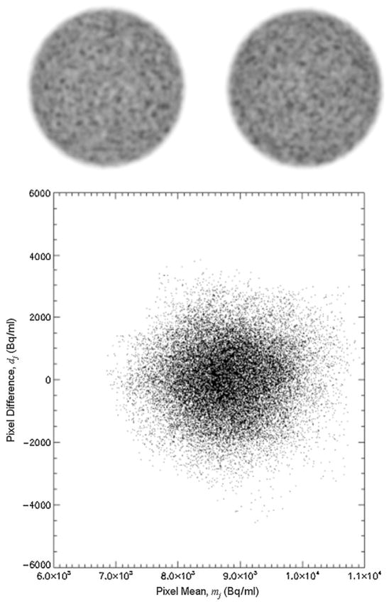
Image noise was calculated by considering only those pixels within a 19 cm diameter circular ROI. The locations of the ROIs were automatically determined so as to be centered in the middle of the phantom in each slice. For all pixels j within the circular ROI, both the difference (d_j) and the mean (m_j) for corresponding pixels in the two replicate images were calculated. Figure 1 shows an example plot of d_j versus m_j for all n pixels within the circular ROI. The standard deviation of d_j over all pixels in the ROI is a measure of image noise and is denoted by dsd_i for slice i:

$${\mathit{dsd}}_i=\sqrt{\frac{n{\displaystyle \sum _j}{d}_j^2-{\left({\displaystyle \sum _j}{d}_j\right)}^2}{n(n-1)}}.$$ (1)

Figure 1.

Corresponding slices from two separately acquired images differ due to statistical noise. This noise is shown graphically in a plot of the difference between corresponding pixels (d_j) as a function of the average of the corresponding pixels (m_j), for all pixels within a 19 cm diameter circular ROI centered on the phantom.

Image noise was expressed as a percentage coefficient-of-variation for each slice and was also averaged over all slices to reflect the overall coefficient-of-variation (COV):

$$\text{COV}=100\times \frac{1}{S\sqrt{2}}\sum _i^S\frac{{\mathit{dsd}}_i}{a_i}$$ (2)

where a_i is the average of m_j for all pixels within the ROI in slice i and S indicates the total number of slices. Note the factor of $\sqrt{2}$ was introduced to account for the fact that dsd_i is the standard deviation of the difference data as opposed to the pixel data itself. This equation can also be reformulated as a signal-to-noise-ratio (SNR) given by

$$\text{SNR}=\frac{\sqrt{2}}{S}\sum _i^S\frac{a_i}{{\mathit{dsd}}_i}.$$ (3)

2.3. Spatial resolution

Spatial resolution was assessed by measuring the extent of the blurring around the edge of the phantom in each of the transaxial images. This method assumed that the cylindrical phantom had a sharp discontinuity at the edge and that the blur observed in the images was a measure of the system spatial resolution. Because the phantom was positioned in the middle of the field-of-view, the edges of the cylinder were all 10 cm from the center and the resolution was expected to be the same for all points around this edge.

Whereas 19 cm diameter circular ROIs were used to measure image noise because the smaller region size minimized edge effects, 20 cm diameter ROIs were used to measure spatial resolution. This ROI size was chosen to exactly match the known diameter of the radioactive portion of the cylinder phantom. The two replicate images were averaged to produce a single image volume with lower noise. The center of the phantom was determined for each slice and 20 cm diameter circular ROIs were positioned in the center of the phantom images. These 20 cm ROIs were used for the purpose of creating a secondary image volume in which all pixels within the ROI were assigned a value of 1 and all pixels outside were assigned a value of 0. In this way, an additional binary image was created that was spatially aligned with the original image volume but had perfect spatial resolution and no image noise. Note that both the original image and the binary image had the same matrix size and included surrounding pixels that extended beyond the edges of the phantom. We denote the original image I and the binary image, or object function, O and we assume that the two are related by a PSF:

$$I(x,y)=O(x,y)\otimes \text{PSF}(x,y)$$ (4)

where ⊗ indicates two-dimensional (2D) convolution. PSF is an unknown 2D function that characterizes the system spatial resolution in the transaxial plane (radial direction) and is dependent on a number of factors including positron range, diameter of detector ring, detector material and size, as well as image reconstruction parameters.

In order to measure PSF, both I and O were rebinned from their original 256 × 256 matrix to a larger 512 × 512 array using linear interpolation so as to produce a 0.5 mm sampling interval. Each slice of the two image volumes were 2D Fourier transformed and data from corresponding slices of I were divided by O in the Fourier domain. The resulting data were inverse Fourier transformed to produce a PSF in real space:

$$\text{PSF}=F^{-1}\left[\frac{F[I]}{F[O]}\right]$$ (5)

where F indicates 2D Fourier transform and F⁻¹ indicates inverse 2D Fourier transform. Spatial resolution was characterized by fitting a 2D Gaussian function to the PSF image and reporting the FWHM of the fitted function. The method was made particularly robust with respect to noise by averaging the PSF images for all slices before performing a single 2D Gaussian fit.

2.4. Method evaluation

2.4.1. Image noise

Noise estimates, determined using the proposed method, were compared with separate measurements derived from multiple statistical replicates. 40 separate acquisitions were performed at nine different noise levels. All data were acquired in 2D mode on the Discovery RX using the previously described 20 cm diameter ⁶⁸Ge cylinder phantom. Each noise level was determined by terminating the acquisition at a specific number of total true counts (1, 2.5, 5, 10, 20, 30, 40, 50, 60 million). At each noise level, the 40 image volumes represented different noise realizations but, in all other respects, were identical. The image signal-to-noise ratio was estimated by applying a single pixel ROI to each noise series and by determining the mean divided by the standard deviation of the 40 pixel values. The SNR determined in this way was averaged over all pixels within a 19 cm diameter circular ROI for all slices (method A). This measure of the SNR was compared with the proposed method using paired images (method B, see subsection 2.2), where each of the paired images comprised the same number of true coincidence counts (1, 2.5, 5, 10, 20, 30, 40, 50, 60 million). In addition, a third estimate of the SNR was obtained by applying the same 19 cm diameter ROI to a single image volume. The SNR was calculated as the mean divided by the standard deviation of all pixels in the ROI (method C). In order to investigate the effect of image non-uniformity, method B was also used to measure the SNR in grossly non-uniform, non-attenuation-corrected images.

The repeatability (Halligan 2002) of the method was estimated by performing a series of ten paired measurements on the Discovery RX in 2D mode. Data were acquired on ten separate days, and at each session, the entire measurement procedure was repeated (a total of four 7.5 min acquisitions). Between each pair of measurements, the phantom was physically moved, repositioned in the center of the field-of-view and a new CT was performed for attenuation correction. Repeatability was measured by calculating the difference between each of the two SNR measurements; determining the standard deviation of these ten difference values; multiplying the resulting standard deviation by 1.96 and expressing it as a percentage of the mean SNR. The difference between two repeated measurements of the SNR is expected to be less than this measure of repeatability for 95% of pairs of observations, under the assumption that the data are normally distributed (Bland and Altman 1996).

2.4.2. Example application

A number of different methods of correcting for random coincidence events have been developed including subtraction of data acquired in a delayed coincidence channel and corrections based on detector singles rates (Brasse et al 2005). The singles-based method is known to produce correction factors with lower noise (Stearns et al 2003) due to the fact that single photon count rates are much greater than coincidence count rates. However, this noise advantage may not be readily apparent in reconstructed images. For instance, figure 2 shows images reconstructed from the same projection data using both delayed event subtraction and singles-based randoms correction. All other processing parameters were identical including the reconstruction algorithm: 3D maximum-likelihood expectation-maximization (ML-EM), 42 iterations and 3 mm post-reconstruction Gaussian filter. Visual inspection of the images suggested that delayed event subtraction, not singles-based correction, gave rise to the image with the lowest noise. This observation was investigated quantitatively using the proposed method of simultaneously measuring noise and spatial resolution. The same 3D projection data, acquired on the Discovery RX and consisting of prompt and delayed sinograms (6.5 ns coincidence timing window), were used to reconstruct different images, using each of the two randoms correction techniques. For each method of randoms correction, a series of images were reconstructed using ML-EM with increasing iterations (iterations = n × 6, where n = 1, …, 14) and the noise versus spatial resolution trade-off was analyzed.

Figure 2.

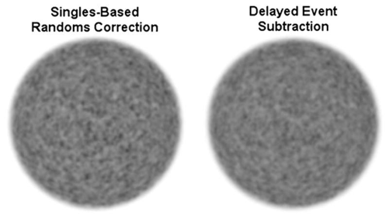
Images reconstructed from the same projection data using singles-based randoms correction (left) and delayed event subtraction (right). All other processing parameters were identical including the reconstruction algorithm: 3D ML-EM, 42 iterations and 3 mm post-reconstruction Gaussian filter. Note no obvious improvement in the statistical quality of the image reconstructed with singles-based randoms correction (left).

3. Results

3.1. Image noise

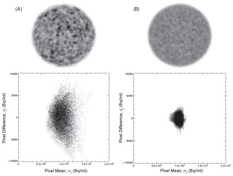
Figure 3 illustrates qualitatively how the standard deviation of d_j reflects image noise. The images in figures 3(A) and (B) were reconstructed from 1 × 10⁶ and 50 × 10⁶ coincidence counts, respectively. Higher noise in the 1 × 10⁶ count image was reflected in figure 3(A) as a broader spread of d_j compared to figure 3(B).

Figure 3.

Images reconstructed from 1 × 10⁶ (A) and 50 × 10⁶ (B) coincidence counts and the corresponding plots of d_j versus m_j. Note that each of the images in (A) and (B) have a corresponding image with different noise (not shown) that was used to produce the data in the graphs.

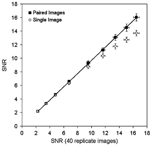
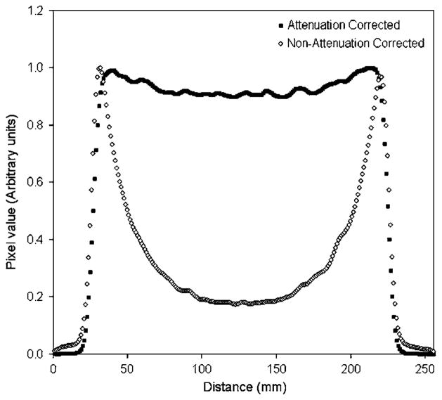
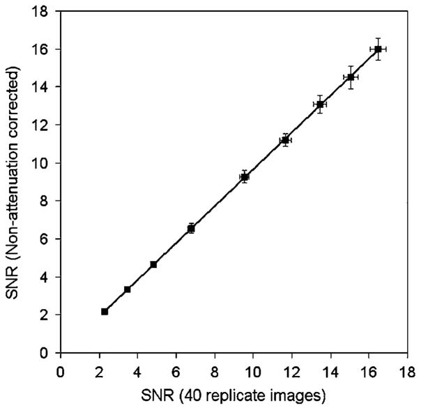
Figure 4 shows SNR data as a function of the signal-to-noise ratio derived from 40 replicate scans (method A), over a range of noise levels. The solid squares indicate results derived from the proposed noise estimation method involving the difference of paired images (method B). The solid line represents a linear fit to these data (y = 0.97x − 0.03) and suggests close agreement between the two methods. On average, the SNR measured using method B was 3.4 ± 0.7% lower than method A. The open circles indicate SNR data derived by dividing the mean by the standard deviation of all pixels in a single image ROI (method C). These data are seen to diverge from method B (and method A) as statistical quality improved. Figure 5 shows line profiles through a typical attenuation-corrected image (used for all data in figure 4) and also a non-attenuation-corrected image. Note that the attenuation-corrected data are slightly non-uniform across the cylinder and shows a 10% decrease in signal at the center compared to the edge. This non-uniformity may account for the underestimated SNR at low noise levels with method C but does not appear to affect method B (see figure 4). In order to further investigate the effect of image non-uniformity on method B, we analyzed the noise in grossly non-uniform, non-attenuation-corrected images. Figure 6 shows the SNR estimated using method B, but in this case pairs of non-attenuation-corrected images were used. Note that the resulting SNR estimates were similar to those derived using method A, despite the fact that the non-attenuation-corrected images were grossly non-uniform. On average, the SNR measured using method B with non-attenuation-corrected images was 3.7 ± 0.9% lower than method A.

Figure 4.

Signal-to-noise ratios determined using three different methods for a range of images with different noise levels (1, 2.5, 5, 10, 20, 30, 40, 50, 60 million total true counts). The data are shown as a function of the SNR estimate obtained from 40 replicate images (method A). Solid squares denote data obtained with the proposed method involving the difference of paired images (method B). Open circles denote the data obtained by simply dividing the mean by the standard deviation of all pixels in a single image ROI (method C). The solid line indicates a linear fit to the data derived from method B (y = 0.97x − 0.03). All images were acquired on the Discovery RX in 2D mode.

Figure 5.

Line profiles drawn in a transverse slice through both attenuation corrected and non-attenuation corrected cylinder images. In addition to the expected non-uniformity in the non-attenuation corrected image, non-uniformity was also observed in the attenuation corrected image. A 10% reduction in reconstructed signal intensity was observed at the center compared to the edge of the phantom. Data acquired in 2D on the Discovery RX.

Figure 6.

Signal-to-noise ratio estimated using the proposed method (method B) in conjunction with non-attenuation corrected images. The data are shown as a function of the SNR estimate obtained from method A with attenuation correction. Data over a range of noise levels are included (1, 2.5, 5, 10, 20, 30, 40, 50, 60 million total true counts). The solid line indicates a linear fit to the data (y = 0.97x − 0.04) and indicates close agreement despite the fact method B used grossly non-uniform non-attenuation corrected images. All data were acquired on the Discovery RX in 2D mode.

Based on the ten replicate measurements, repeatability of the SNR using method B was 0.83%. That is to say that two sequential measurements of the SNR are expected to differ by less than 0.83%, for 95% of observations.

3.2. Example application

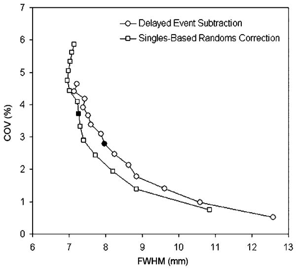
Figure 7 shows a graph of noise (COV) versus spatial resolution (FWHM) for images reconstructed with different numbers of iterations, using both delayed event and singles-based randoms corrections. The two data points marked with solid symbols denote the images shown in figure 2 (both reconstructed with 42 iterations). It can be seen from the graph that, although the image corrected using delayed event subtraction had lower noise than the corresponding singles-based correction image, this was obtained at the expense of poorer spatial resolution. When the two randoms-correction schemes were compared at a fixed spatial resolution, the singles-based method gave rise to images with lower noise. Using the proposed method of simultaneously measuring spatial resolution and noise, the singles-based randoms correction was seen to both reduce image noise (for matched spatial resolution) and increase the speed of convergence of the iterative reconstruction algorithm. The higher noise observed after 42 iterations (and suggested in the images in figure 2) using singles-based randoms correction was therefore seen to be a consequence of the faster convergence rate of the iterative reconstruction when using this method of randoms correction.

Figure 7.

Image noise (COV) plotted against spatial resolution (FWHM) for 6, 12, 18, 24, 30, 36, 42, 48, 54, 60, 66, 72, 78, 84 iterations (right to left). Circles indicate randoms correction using delayed event subtraction. Squares indicate singles-based randoms correction. All other processing parameters were identical. The two solid data points correspond to the images shown in figure 2. The true coincidence count rate was 875 kcps and the random coincidence rate was 589 kcps.

4. Discussion

Many centers routinely use ⁶⁸Ge cylinder phantoms to assess detector performance and to check the quantitative accuracy of reconstructed images. In this paper we show that additional information regarding spatial resolution and image noise can also be obtained from these data. The proposed method allows spatial resolution and image noise to be measured simultaneously and may have applications evaluating new algorithms or new software implementations. This latter application is of practical significance as manufacturer’s upgrades to scanner software sometimes have unexpected consequences for existing protocols. Additionally, the method can be used to characterize different clinical protocols and, because it can be applied to images acquired on all PET systems, it may help to standardize procedures between institutions. Such standardization is critically important for longitudinal multi-center studies, especially if varying types of equipment are used.

One of the advantages of our method of calculating noise is that only two statistically independent images are required. Conventional methods require multiple statistical replicates which is often difficult to obtain, even with phantom data. Figure 4 confirms that the proposed noise estimation method produced results in close agreement with those from multiple replicate images, which served as a reference for noise estimation. Taking the difference between corresponding pixels allowed noise to be measured even if the images had pronounced nonuniformity. This is confirmed in figure 6 which shows that the SNR measured from grossly non-uniform, non-attenuation corrected images was similar to the reference obtained from 40 replicate attenuation corrected images. The purpose of including the non-attenuation corrected data was to illustrate that the method of measuring noise did not require the underlying image data to be perfectly uniform. This property may be of practical importance as it allows noise to be measured in cases where the image uniformity is known to be imperfect. Such nonuniformity may be due to imperfect attenuation or scatter correction and is not uncommon (see figure 5). Furthermore, this property eliminates uncertainty due to the construction of the ⁶⁸Ge phantom, which is not expected to have a perfectly uniform distribution. Note that estimating noise by simply determining the standard deviation of pixels within a large ROI assumes perfect image uniformity. For experimental data this is not usually a realistic assumption and may account for the underestimation of the SNR (overestimation of the standard deviation of pixels within the ROI) in figure 4 for the low-noise images where non-uniformity becomes more significant.

It is expected that correlations between nearby pixels could potentially bias noise estimation using the proposed method of subtracting paired images. Although each image is statistically independent, adjacent pixels in the same image will be highly correlated, especially after the application of a post-reconstruction smoothing filter. Given these correlations, the differences between corresponding pixels in paired images are also expected to be correlated for nearby pixels. Despite these correlations, figure 4 shows that the SNR measurements were in close agreement with those obtained using multiple replicates. This is likely due to the fact that although some pixels were correlated, the 19 cm diameter ROI contained many spatially separate pixels that were not significantly correlated, allowing accurate estimation of the standard deviation. Note that modifications of this method that use smaller ROIs may be susceptible to bias due to pixel correlation.

In the example of different randoms correction schemes, we saw that, unless both image noise and spatial resolution were measured simultaneously, misleading conclusions could be drawn. When the reconstruction parameters were identical, delayed event subtraction gave rise to lower image noise than the singles-based correction. This finding was unexpected, as the singles-based correction factors are known to have much lower noise than the corresponding data obtained from the delayed coincidence channel. However, when noise and resolution were measured as a function of iterations, it was found that the iterative reconstruction algorithm converged faster when singles-based randoms correction was applied. It can be seen in figure 7 that, for a fixed number of iterations, noise was lower with delayed event subtraction, but this was obtained at the expense of poorer spatial resolution. Although unexpected, and not obvious from the images shown in figure 2, the method of randoms correction was found to indirectly influence spatial resolution when iterative image reconstruction was employed. The singles-based randoms estimate was modeled in the iterative loop, whereas the delayed coincidence data were subtracted from the prompt data prior to image reconstruction, as would be the case with online subtraction of delayed events. The effect of including the randoms correction in the loop was to accelerate the convergence of the algorithm, as the Poisson properties of the data were better preserved. When a fixed spatial resolution was considered, as opposed to a fixed number of iterations, the singles-based randoms correction gave rise to lower noise than delayed-event subtraction. This was because, when resolution was matched, the two algorithms could be compared in an unbiased fashion and the better statistical quality of the singles-based randoms estimate became apparent. The proposed method of simultaneously measuring noise and resolution allows trade-offs of this sort to be accurately quantified in a very convenient manner.

5. Conclusion

A phantom procedure has been developed that allows simultaneous measurement of image noise and spatial resolution. The proposed method is useful for evaluating reconstruction algorithms and may aid standardization of data collection between centers.

References

- Bergstrom M, Eriksson L, Bohm C, Blomqvist G, Litton J-E. Correction for scattered radiation in a ring detector positron camera by integral transformation of the projections. J Comput Assist Tomogr. 1983;7:42–50. doi: 10.1097/00004728-198302000-00008. [DOI] [PubMed] [Google Scholar]
- Bland JM, Altman DG. Statistics notes: measurement error. BMJ. 1996;313:744. doi: 10.1136/bmj.313.7059.744. [DOI] [PMC free article] [PubMed] [Google Scholar]
- Brasse D, Kinahan PE, Lartizien C, Comtat C, Casey M, Michel C. Correction methods for random coincidences in fully 3D whole-body PET: impact on data and image quality. J Nucl Med. 2005;46:859–67. [PubMed] [Google Scholar]
- Halligan S. Reproducibility, repeatability, correlation and measurement error. Br J Radiol. 2002;75:193–4. doi: 10.1259/bjr.75.890.750193. [DOI] [PubMed] [Google Scholar]
- Hudson HM, Larkin RS. Accelerated image reconstruction using ordered subsets of projection data. IEEE Trans Med Imaging. 1994;13:601–9. doi: 10.1109/42.363108. [DOI] [PubMed] [Google Scholar]
- Kadrmas DJ, Christian PE. Comparative evaluation of lesion detectability for 6 PET imaging platforms using a highly reproducible whole-body phantom with 22Na lesions and localization ROC analysis. J Nucl Med. 2002;43:1545–54. [PubMed] [Google Scholar]
- Kemp BJ, Kim C, Williams JJ, Ganin A, Lowe VJ. NEMA NU 2-2001 performance measurements of an LYSO-based PET/CT system in 2D and 3D acquisition modes. J Nucl Med. 2006;47:1960–7. [PubMed] [Google Scholar]
- Liow J-S, Strother SC. The convergence of object dependent resolution in maximum likelihood based tomographic image reconstruction. Phys Med Biol. 1993;38:55–70. doi: 10.1088/0031-9155/38/1/005. [DOI] [PubMed] [Google Scholar]
- Lodge MA, Rahmim A, Wahl RL. A practical, automated quality assurance method for measuring spatial resolution in PET. J Nucl Med. 2009;50:1307–14. doi: 10.2967/jnumed.108.060079. [DOI] [PMC free article] [PubMed] [Google Scholar]
- Mawlawi O, Townsend DW. Multimodality imaging: an update on PET/CT technology. Eur J Nucl Med Mol Imaging. 2009;36:S15–29. doi: 10.1007/s00259-008-1016-6. [DOI] [PubMed] [Google Scholar]
- NEMA. Performance Measurements of Positron Emission Tomographs NU 2-2007. Rosslyn, VA: National Electrical Manufacturers Association; 2007. [Google Scholar]
- Ollinger JM. Model-based scatter correction for fully 3D PET. Phys Med Biol. 1996;41:153–76. doi: 10.1088/0031-9155/41/1/012. [DOI] [PubMed] [Google Scholar]
- Qi J, Leahy RM. Iterative reconstruction techniques in emission computed tomography. Phys Med Biol. 2006;51:R541–78. doi: 10.1088/0031-9155/51/15/R01. [DOI] [PubMed] [Google Scholar]
- Stearns CW, McDaniel DL, Kohlmyer SG, Arul PR, Geiser BP, Shanmugam V. Random coincidence estimation from single event rates on the Discovery ST PET/CT scanner. IEEE Nucl Sci Symp Conf Rec. 2003:3067–9. [Google Scholar]
- Tang J, Rahmim A, Lautamaki R, Lodge MA, Bengel FM, Tsui BMW. Optimization of Rb-82 PET acquisition and reconstruction protocols for myocardial perfusion defect detection. Phys Med Biol. 2009;54:3161–71. doi: 10.1088/0031-9155/54/10/013. [DOI] [PMC free article] [PubMed] [Google Scholar]