Next Generation Sequence Assembly with AMOS

Abstract

A Modular Open-Source Assembler (AMOS) was designed to offer a modular approach to genome assembly. AMOS includes a wide range of tools for assembly, including lightweight de novo assemblers Minimus and Minimo, and Bambus 2, a robust scaffolder able to handle metagenomic and polymorphic data. This protocol describes how to configure and use AMOS for the assembly of Next Generation sequence data. Additionally, we provide three tutorial examples that include bacterial, viral, and metagenomic datasets with specific tips for improving assembly quality.

INTRODUCTION

Over three decades ago, a highly influential work published by Fred Sanger and Alan R. Coulson on the rapid determination of DNA sequence (Sanger et al. 1975) helped pave the way for the arrival of the first sequenced bacterial genome via whole-genome shotgun (WGS) sequencing in 1995 (Fleischmann et al. 1995). Whole-genome shotgun sequencing is a technique in which large pieces of DNA from genomes are randomly sheared into smaller fragments that are then cloned and sequenced. The goal of sequence assembly is to take the shotgun-sequenced reads and recover the original whole genome. In contrast with comparative assemblers (which rely on a closely-related reference sequence), de novo assemblers have the ability to reconstruct organisms that have no sequenced close relatives or that contain novel gene content. This is especially important for environmental strains and metagenomic projects. The main piece of evidence for assembling the reads into the original genome is the overlap between segments of these reads. Unfortunately, sequencing errors and repeated regions make assembly a challenging problem. Mate-pairs, or paired-end reads, sequenced at a known distance from each other, provide additional clues for improving assemblies. Higher redundancy of sequenced regions, i.e. generating thousands or even millions of reads, also ensures that overlaps exist and that a consensus sequence can be generated.

With the advent of massively-parallel high-throughput sequencing that is able to produce millions of bases in a few hours (Margulies et al. 2005), reads became significantly smaller and more error prone but at the same time genome coverage was dramatically increased. Currently, it is common to sequence genomes with the Illumina technology, which yields 35-100 bp length reads from fragments with a 200-300 bp insert size. Genome coverage represents the amount by which the total amount of sequence in the shotgun reads exceeds the actual size of the genome being sequenced. Traditionally, genomes were sequenced to about 8-10-fold coverage; however, next generation sequencing (NGS) projects routinely generate in excess of 20-fold coverage. Two lanes of Illumina 35 bp reads sequenced from Escherichia coli K12 would generate nearly 220-fold of genome coverage!

With the rapid advent of such voluminous data, there is great demand for de novo assemblers able to handle NGS data (J. R. Miller et al. 2010; Nagarajan et al. 2010). The properties of NGS data, however, create new challenges compared to first generation Sanger sequencing, some which make assembly more computationally demanding and others which reduce assembly quality (Pop et al. 2008; Michael C Schatz et al. 2010). There are two main paradigms used for assembly. The first, called Overlap-Layout-Consensus relies on an overlap graph (Eugene W Myers 2005). A graph is a common abstraction in computer science. It contains a set of nodes and edges, indicating connections between nodes. An overlap graph’s nodes are the reads, and the edges represent end-end shared sequence between reads. The second paradigm is based on a de Bruijn graph (Idury et al. 1995; Pevzner et al. 2001), a data structure where nodes typically represent fixed-length strings drawn from a larger set of strings (the reads) and edges represent perfect shared sequences. In both cases, a series of algorithms are applied to simplify the graph and produce an assembly. The computational complexity of Overlap-Layout-Consensus -based assemblers has increased with NGS as the total number of overlaps for resolving the assembly puzzle (assuming uniform read distribution) is approximately equal to (Len_genome − Len_read) X Coverage_genome X 2, which can quickly translate into millions of overlaps. Assemblers based on the de Bruijn algorithm scale better with respect to the number of reads — the size of the underlying data structure is, in theory, proportional to the size of the genome and independent of the actual number of reads generated in the sequencing experiment (Unit 11.5; Zerbino et al. 2008). De Bruijn graph-based assemblers, however, have difficulties handling sequencing errors, and in practice, assembly of large genomes still requires the use of plenty of processors and memory (100 GB+). With respect to assembly quality, many issues come into play, such as: (1) sequencing errors (human and technology), (2) uneven genome coverage, and (3) reads too short to span repeated regions. Recent methods have been developed to address the various shortcomings of (1) (Zhao et al. 2010; Yang et al. 2010; Salmela 2010), while (2) and possibly (3) can be addressed by using a combination of many short reads and fewer longer reads, e.g. by using Sanger, 454 and Illumina sequencing simultaneously (Dalloul et al. 2010).

In this protocol we will start by describing Minimus (Sommer et al. 2007), a lightweight assembler included in the AMOS software package. Minimus was designed specifically for small datasets, such as the set of reads covering a single gene or virus. Note that Minimus can be applied to larger-scale assemblies (e.g. to assemble large bacterial genomes and metagenomic data);; however, due to its stringency, the resulting assembly will often be highly fragmented. Another assembler part of AMOS is Minimo. Assembly stringency can be changed in Minimo, allowing for a very granular approach to genome assembly. However, for larger or complex genomes the execution of Minimus and Minimo should be followed by additional processing steps, such as scaffolding via Bambus (Pop et al. 2004), or incorporated into more complex assembly pipelines (Kislyuk et al. 2010). Both Minimus and Minimo follow the Overlap-Layout-Consensus paradigm (Eugene W Myers 2005) and consist of three main modules which share information through a central file bank (Figure 11.8.1): (1) the hash-overlap module computes the overlap between pairs of reads using a modified version of the Smith-Waterman local alignment algorithm;; (2) the tigger module then uses these overlaps to find the arrangement of reads in individual contigs, using the algorithms described by Myers;; and (3) the make-consensus module refines the layouts by performing a multiple alignment of the reads in each contig to produce accurate consensus sequences. Minimus, Minimo, and Bambus 2 all use the open AMOS message format for communication. Both, the overall modular structure of the AMOS package and the general structure of the files used to communicate between individual modules were broadly inspired by the design of Celera Assembler (E. W. Myers 2000).

Figure 11.8.1.

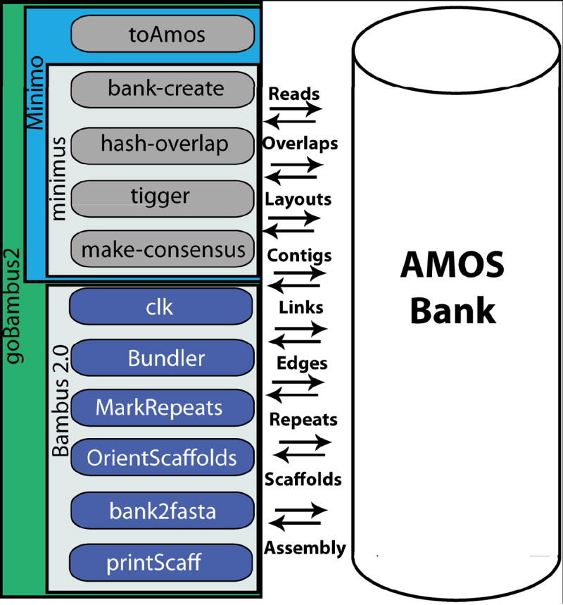
Overview of the AMOS assembly pipeline. On the left-hand side we see the various AMOS assembly pipelines and modules, including: Minimus/Minimo, and Bambus 2.0/goBambus2. On the right-hand side we see the interaction between each individual module and the AMOS bank, a database that stores the reads, overlaps, layouts, contigs, contig links, contig edges, repeats, scaffolds and assembly information.

The three tutorials that follow will delve into further details on how to use AMOS to assemble viruses, bacteria and metagenomic data.

BASIC PROTOCOL 1

ASSEMBLY OF A SMALL BACTERIAL GENOME

This protocol describes the steps involved in running Minimus on a small dataset. As a first example we will explain how to assemble simulated reads generated from the smallest bacterial genome known, Candidatus Carsonella ruddii, using Minimus. This example contains 32,000 100-bp reads simulated using the open-source simulator Grinder (http://sourceforge.net/projects/biogrinder) (Angly et al. 2009), resulting in 20X coverage of this genome. These reads are available in the AMOS package.

The purpose of this example is to demonstrate how straightforward it is to generate and visualize an assembly with Minimus and Hawkeye. However, this is not a realistic example as the reads are error-free and uniformly distributed across the genome. Basic protocols 2 and 3 involve more realistic assembly examples, with paired-end reads that include sequencing errors and a simulated metagenomic dataset. This will make the assembly problem much more challenging, requiring manual adjustment of the assembly parameters to achieve a better assembly.

Necessary Resources

Hardware

A computer with at least 4 GB of RAM with a modern version of UNIX installed.

Software

Minimus. This is distributed under an Open Source license as a component of the AMOS package: http://sourceforge.net/projects/amos/. Minimus and AMOS Installation Instructions can be found in Support Protocol 1.

Files

Candidatus Carsonella ruddii FASTA sequence of the reads (c_ruddii.seq).

• Note: In order to run Minimus you need to provide an AMOS-formatted read file. Such a file (commonly with the .afg extension) can be generated directly from the sequence file using the toAmos tool, as will be described later in this protocol.

In the following examples, the command line prompt is indicated as “>”. User input is bold face, and output from the command is given in regular weight font.

1. From the command line, enter the AMOS tutorial directory by typing:

   > cd ./tutorial/minimus

   • The test directory contains four datasets for tutorial purposes. It is located within the AMOS project.

2. To see the tutorial directory examples type:

   > ls

   • There are three example subdirectories inside of the test directory:

     • bacterium
     • bacteriophage
     • metagenome

   • The CVS directories can be ignored, they are used for version control of the AMOS project and do not form part of the tutorial.

3. Start the first example by entering the bacterium directory:

   > cd bacterium

4. List the example files:

   > ls

5. Confirm that the following required files are present:

   c_ruddii.seq: Reads in FASTA format

6. Run toAmos to prepare AMOS formatted input file for Minimus:

   > toAmos -s c_ruddii.seq -o c_ruddii.afg

7. Now run the minimus pipeline with default parameter values and settings:

   > minimus c_ruddii

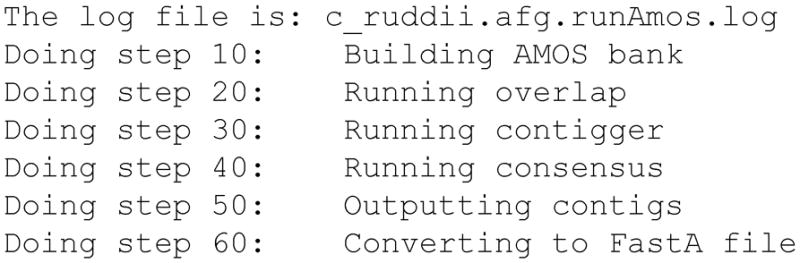
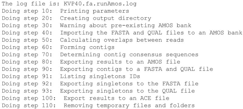
   • This command will automatically run bank-transact, hash-overlap, tigger, and make-consensus, in that order. For further details see next section on running each step individually. A log file will be created and the output shown in Figure 11.8.2 will appear.

   • When Minimus successfully completes the job, the following output files will be created:

     • c_ruddii.bnk: AMOS databank
     • c_ruddii.fasta: Minimus assembly in FASTA format
     • c_ruddii.contig: Minimus assembly in TIGR format

   • Output will be a TIGR .contig file and a FastA .fasta file. The TIGR contig file contains the gapped consensus and multi-alignment information for the assembly. Each contig sequence is preceded by a header line which starts with ‘##’, followed by the gapped consensus sequence with gaps represented as a ‘-’ character. Following the consensus is the gapped read sequence preceded by a header line beginning with ‘#’. The .fasta file contains all the contigs produced by Minimus in a multi-FastA formatted file. These sequences match the sequences in the .contig file, but without the gaps.

8. View the contigs resulting from assembly:

   > grep ## c_ruddii.contig

   Inspection of the c_ruddii.contig file reveals that Minimus assembled this dataset into a single contig (Figure 11.8.3).

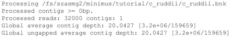
9. To get a summary of read coverage of this single contig:

   > analyze-read-depth c_ruddii.bnk (Figure 11.8.4)

10. To visualize the assembly and reads using Hawkeye (Michael C Schatz et al. 2007) run the following command (Figure 11.8.5):

    > hawkeye c_ruddii.bnk

11. Click on the “Scaffold View” icon for a graphic representation of the position of the reads in the genome scaffold.

Figure 11.8.2.

Screenshot of Minimus output

Figure 11.8.3.

Screenshot of C. ruddii assembled contigs

Figure 11.8.4.

Screenshot of analyze-read-depth output

Figure 11.8.5.

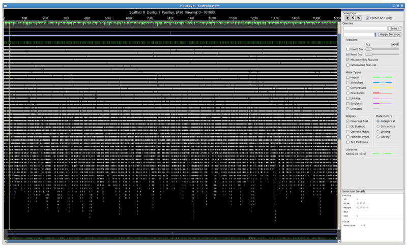
Visualization of an assembly with Hawkeye.

BASIC PROTOCOL 2

ASSEMBLY OF A PHAGE GENOME

In this example we will assemble a T4-like bacteriophage (Genbank Accession AY283928) with a 245 kb long genome from 454 GS-FLX reads (220 bp on average, with homopolymer errors, 40x genome coverage) simulated using Grinder. These errors will result in a more fragmented assembly than in the previous example, but are more representative of real data. To address this we will run Minimo. Minimo uses the same Overlap-Layout-Consensus (OLC) algorithm as Minimus but allows users to specify the desired minimum overlap length and identity. We will improve the assembly by decreasing the minimum percent identity and increasing the minimum overlap length parameter a step at a time.

Necessary Resources

Hardware

A computer with at least4 GB of RAM with a modern version of Unix installed

Software

Minimo, getN50 and Bambus 2.0

Files

FASTA simulated paired reads of bacteriophage KVP40 reads (KVP40.fa)

1. From the command line enter the bacteriophage example directory by typing:

   > cd ./tutorial/minimus/bacteriophage

2. List the example files:

   > ls

3. Confirm that the following file is present:

   KVP40̷.fa

4. Display the manual for Minimo (Figure 11.8.6):

   > Minimo -h

   • Unlike Minimus, Minimo integrates the toAmos step such that the input file can simply be a FASTA file.

5. Generate an assembly with Minimo (Figure 11.8.7):

   > Minimo KVP40.fa -D MIN_LEN=40 -D MIN_IDENT=98 -D FASTA_EXP=1

   • When Minimo imports reads using toAmos, reads with identical identifiers ending in /1 or /2 will be automatically recognized as mate-pairs. While Minimus and Minimo do not use mate pair information for the assembly, this will be essential for scaffolding. For the assembly part, we request here that reads overlap by at least 40 bp and are at least 96% identical in order to be placed inside the same contig. We also specify that contigs in the AMOS bank should be exported in a FASTA format. The ACE format, a widely used assembly format is also available for downstream analysis with external programs.

   • At the end of the Minimo step, the following output files will be created:

     • KVP40-contigs.afg: Minimo assembly in AMOS format
     • KVP40-contigs.fa: Minimo assembly in FASTA format
     • KVP40-contigs.qual: Quality scores for the Minimo assembly
   • Note: This single Minimo step could be replaced by the following AMOS commands:

     • > toAmos -s KVP40.fa -o KVP40.afg
     • > bank-transact -cf -m KVP40.afg -b KVP40.bnk
     • > hash-overlap -x 0.04 -o 40 -b KVP40.bnk
     • > tigger -b KVP40.bnk
     • > make-consensus -e 0.04 -o 40 -b KVP40.bnk
     • > bank2fasta -b KVP40.bnk > KVP40-contigs.fa

   • Note: Many AMOS utilities, including Minimus and Minimo, are simply text files specifying the parameters for the individual commands within the assembly pipeline. These files can be easily modified in order to adapt them to specialized settings. To view the contents of Minimo, for example, simply type:

     > more ‘which Minimo’

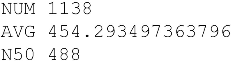
6. To evaluate the quality of the assembly one can compute the N50 measure, which represents the contig length L such that contigs equal or longer than L contain 50% of the bases in the genome. To calculate this and other assembly statistics, run:

   > getN50 KVP40-contigs.fa (Figure 11.8.8)

   • These numbers illustrate that the assembly is poor, given that there are still over 1,000 contigs and that the N50 and average contig size are only twice the read length. This is most often the result of a combination of (a) unequal read coverage, (b) high repeat content and (c) errors in the reads.

7. Decrease the minimum overlap similarity from 98% to 97% to try to assemble more reads that can contain sequencing errors.

   > Minimo KVP40.fa -D MIN_LEN=40 -D MIN_IDENT=97 -D FASTA_EXP=1

8. View the statistics again (Figure 11.8.9).

   > getN50 KVP40-contigs.fa

   • The assembly is now much less fragmented: the number of contigs has decreased by an order of magnitude and the N50 has increased by two orders of magnitude.

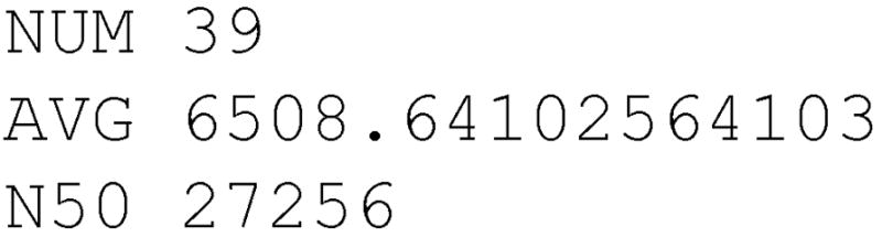
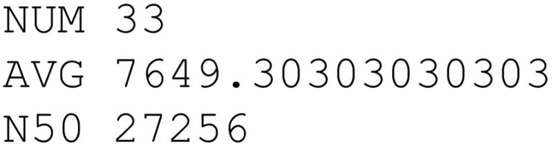
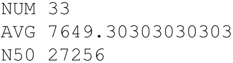
9. Increasing the minimum overlap length from 40 to 80 bp might resolve some small repeats and improve the assembly:

   > Minimo KVP40.fa -D MIN_LEN=80 -D MIN_IDENT=97 -D FASTA_EXP=1

10. Now retrieve the assembly statistics (Figure 11.8.10).

    > getN50 KVP40-contigs.fa

    • An additional six contigs have been joined thanks to the increase in overlap length. So, via two simple parameter changes we have achieved an assembly with a few dozen contigs and N50 size > 27 kb. These unambiguous contigs (unitigs) will provide a useful starting point for scaffolding, as we will now describe.

11. Produce a bank for scaffolding using Bambus 2.

    > bank-transact -cf -m KVP40-contigs.afg -b KVP40.bnk

    • The parameter -cf indicates to forcefully create the bank if one with the same name already exists, -b specifies the bank directory and -m the AMOS input file.

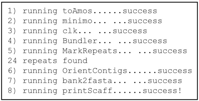
12. While there is a convenience script provided for scaffolding (goBambus2.py), we will proceed via the modules clk, Bundler, OrientContigs, bank2fasta and printScaff. These modules irreversibly modify the bank. If you wish to create a backup of the current bank, do so before proceeding. First, Create links between contigs and mate-pairs (or paired-end reads).

    > clk -b KVP40.bnk

13. Bundle links into edges among connected contigs.

    > Bundler -b KVP40.bnk

14. Find repetitive contigs and mark as repeats.

    > MarkRepeats -b KVP40.bnk > repeats.out

15. Determine contig order and orientation.

    > OrientContigs -b KVP40.bnk -noreduce -linearize -prefix phageScaff

16. Extract fasta formatted contigs from bank.

    > bank2fasta -b KVP40.bnk > phageScaff.contigs.fasta

17. Print scaffold sequence and statistics.

    > printScaff -e phageScaff.evidence.xml -s phageScaff.out.xml -l phageScaff.library -f phageScaff.contigs.fasta -merge -o phageScaff

18. The pipeline has successfully finished. Now to list the output files associated to the scaffold:

    > ls phageScaff*

    • Here is a description of each of these output files:

      1. phageScaff.agp: scaffolds generated by the OrientContigs programs in NCBI AGP format
      2. phageScaff.dot: scaffolds generated by the OrientContigs program in Graphviz dot format
      3. phageScaff.evidence.xml: XML representation of the linking evidence (library and read pairing information, and read placement within each contig, also see AMOS website).
      4. phageScaff.library: mapping from library names (provided by the user) to internal AMOS identifiers.
      5. phageScaff.out.xml: XML representation of scaffolds generated by the OrientContigs program
      6. phageScaff.fasta: Fasta file of the scaffolds, joined by Ns
      7. phageScaff.stats: statistics on the scaffolds generated, including N50 and total span.

    • Bambus 2.0 reports the phage inside a single scaffold and the final genome size as 244,758 bp, while the actual genome size of bacteriophage KVP40 is 244,834 bp. There is a small gap of approx 76 bp in the assembly that likely could be closed via manual inspection or alignment against a reference genome.

Figure 11.8.6.

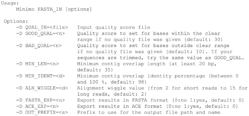
Screenshot of Minimo usage and options.

Figure 11.8.7.

Screenshot of Minimo output.

Figure 11.8.8.

Screenshot of the number of contigs, average contig length and N50 calculated by getN50.

Figure 11.8.9.

Screenshot of the assembly statistics generated with getN50.

Figure 11.8.10.

Screenshot of the assembly statistics generated with getN50.

BASIC PROTOCOL 3

METAGENOMIC EXAMPLE ASSEMBLY

This protocol describes the steps involved in running goBambus2.py on Illumina and 454 reads simulated from metagenomic data. In this example we will show how we can use Minimus and Bambus 2.0 to generate assemblies of a simple metagenomic example containing the previous two examples, one dominant bacteriophage with 40X coverage and a bacterium with 20X coverage.

Necessary Resources

Hardware

A computer with at least= 4 GB of RAM with a modern version of Unix installed

Software

Minimus, Bambus 2.0, goBambus2.py

Files

Combined file containing metagenomic reads simulated in previous protocols

1. From the command line, enter the metagenomic example directory by typing:

   > cd ./tutorial/minimus/metagenome

2. List the example files:

   > ls

3. Confirm the following required files are present:

   combined.fa

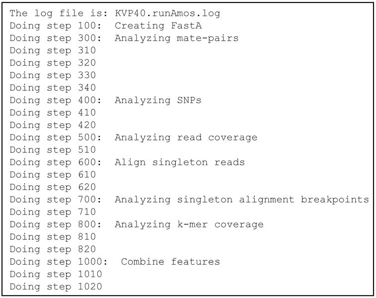
4. Now, run the Bambus pipeline via the following command (Figure 11.8.11):

   > goBambus2.py combined.fa meta2 -all -reads

   • goBambus2.py is an executive script for Bambus. Its purpose is to handle the various input formats and run the necessary AMOS modules for metagenomic and polymorphic assembly. The metagenomic parameter indicates to the script that we would like to assemble metagenomic data and will trigger the use of Minimus with preconfigured parameters.

   • Once goBambus2.py has finished we are ready to inspect the output and determine how much of each genome we assembled. Since this example is generated from simulated datasets and we know the correct answer, we can simply compare the scaffolds to the reference genomes, calculate genome coverage, and inspect assembly quality. See Table 1 for further details.

   • In summary, while this is just a small example and is not representative of an actual metagenomic dataset, it does show that one can extract reasonably good assemblies from a mixture of organisms, even from mixed read types including Illumina and 454 reads.

Figure 11.8.11.

Screenshot of goBambus2.py output.

SUPPORT PROTOCOL 1

DOWNLOADING AND INSTALLING AMOS

This protocol provides instructions for downloading and installing the AMOS software package.

Additional Necessary Resources (see Basic Protocol 1)

Files

Wiki documentation: http://sourceforge.net/apps/mediawiki/amos/index.php?title=AMOSAMOS download link: http://sourceforge.net/project/showfiles.php?group_id=134326

1. Download the Wiki documentation and AMOS source package (see Necessary Resources).

   • The AMOS source package has a name like: amos-3.0.0.tar.gz where 3.0.0 is the version of the code. Once you untar this file (using “tar -xzf amos-3.0.0.tar.gz” in Linux, or “gunzip -d amos-3.0.0.tar.gz | tar xf -” in other flavors of Unix) you will find the current AMOS distribution in a directory named amos-3.0.0. The next steps assume you have cd’d into this directory. AMOS uses the GNU autoconf package to reduce cross-platform compatibility issues.

   • NOTE: If you have downloaded the latest AMOS version from the CVS tip, run the following command before running configure:

     > ./bootstrap

2. After successfully downloading the required files, start the install process by running:

   > ./configure --prefix=/usr/local

   • This probes your system for the locations of all software packages required by AMOS. The --prefix option indicates that the AMOS directory hierarchy will ultimately be installed underneath /usr/local/.

3. Then run make & install:

   ≫ make install

   • Your installation is now complete. The AMOS executables are available under /usr/local/bin. You can verify the installation by running toAmos -h.

   • NOTE: if you do not have root access (required for installation in /usr/local), simply select a directory for which you have permissions and perform a local installation instead:

   • B: Local Installation. This will install AMOS so only you have access to it.

     > ./configure --prefix=~/AMOS

     > make install

   • Your installation is now complete. The AMOS executables are available under ~/AMOS/bin. You can verify the installation by running ~/AMOS/bin/toAmos -h.

   • As a final note, make sure you check the messages left on your screen to make sure no errors occurred. Errors during the configure step can lead to an incomplete build and the program not running properly. If you happen to encounter errors during configuration or compilation, please contact the AMOS development team through the mailing list: amos-help@lists.sourceforge.net

SUPPORT PROTOCOL 2

MODIFYING THE MINIMUS/MINIMO PIPELINE

This protocol provides instructions for modifying the Minimus/Minimo pipelines via the command line. The Minimus/Minimo programs are a compilation of AMOS modules organized inside a file as a pipeline that is executable via the runAmos command.

Necessary Resources

Hardware

A computer with at least 4 GB of RAM with a modern version of Unix installed

Software

Minimus/Minimo

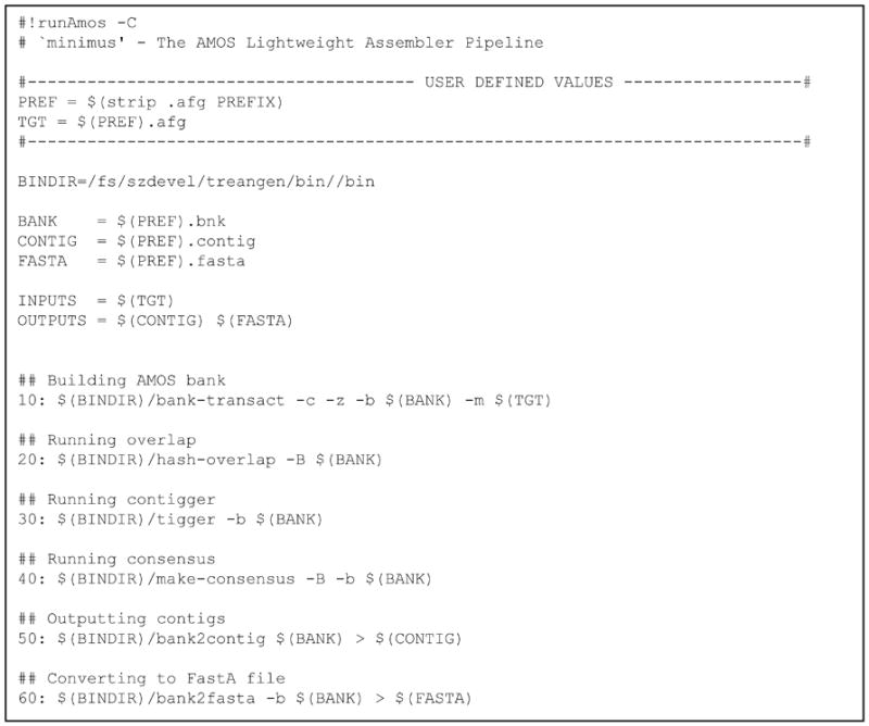
1. View the contents of Minimus (Figure 11.8.12)

   > more minimus

   • All lines that begin with ‘#’ are treated as comments (Figure 11.8.12). Lines starting with numbers increasing in increments of 10 are commands that will be executed in sequential order by runAmos. In the minimus pipeline there are 6 commands executed sequentially. We can add any command we like by simply adding an additional line inside of the file, or remove any module by commenting the line out with ‘#’. Comments starting with ‘##’ are output to the screen before the subsequent command is executed. The user can run just a subset of the commands using options –s start and –e end, as follows:

     > minimus -s 30 -e 50 c_rudii

   • Only commands 30 through 50 will be executed.

Figure 11.8.12.

Screenshot of the modules comprising the minimus pipeline

SUPPORT PROTOCOL 3

VALIDATING AN ASSEMBLY INSIDE AMOS

This protocol provides instructions for validating assemblies and assembly forensics for detecting misassemblies. We will reuse the example from Basic Protocol 2 to show the AMOS tools available for inspecting and validating assemblies, also useful for detecting misassembles.

Necessary Resources

Hardware

A computer with at least 4 GB of RAM with a modern version of Unix installed

Software

Hawkeye, amosvalidate

Files

FASTA simulated paired reads of bacteriophage KVP40 reads (KVP40.fa) from Basic Protocol 2.

• 1Start by entering the assembly directory:

  > cd ./tutorial/minimus/bacteriophage

• 2List the assembly files:

  > ls KVP40*

• 3Confirm the following required fileis present:

  KVP40.bnk

• 4To evaluate the quality of the assembly one can compute the N50 measure, which represents the contig length L such that contigs equal or longer than L contain 50% of the bases in the genome (Figure 11.8.13). To calculate this and other assembly statistics, run

  > getN50 KVP40-contigs.fa

• 5Interactively view the reads, contigs and scaffolds using Hawkeye:

  > hawkeye KVP40.bnk

• 8Run amosvalidate with default parameter values and settings (Figure 11.8.14):

  > amosvalidate KVP40

  • Using the output from the various steps of the amosvalidate pipeline, we will now be able to more carefully analyze and interpret the generated assemblies within AMOS. Amosvalidate generates a collection of “features” representing regions of the assembly that may contain errors. These regions are highlighted in the Hawkeye display.

Figure 11.8.13.

Screenshot of the number of contigs, average contig length and N50 calculated by getN50.

Figure 11.8.14.

Screenshot of amosvalidate output

GUIDELINES FOR UNDERSTANDING RESULTS

In all the examples presented in this unit we generated FASTA formatted sequences representing a given genomic sequence assembly. When a benchmark reference assembly is known, the task of interpreting and evaluating assembly quality is straightforward. However, in de novo assembly a straightforward measure of correctness or accuracy is more challenging. Traditionally, metrics such as N50 values of contigs and unitigs (provided in AMOS by getN50), number of contigs, and maximal contig size are commonly used for understanding the results and often used when evaluating continuity and accuracy. Detection of misassembles such as chimeric contigs is also useful for evaluating the trustworthiness of a given assembly. More advanced techniques include closely analyzing mate-pair information, unused read information, and also correlated polymorphisms. AMOS provides tools for more in-depth analysis and inspection of assemblies generated by assemblers such as Minimus/Minimo and also can be used in conjunction with most existing assemblers thanks to the wide array of conversion tools that AMOS offers (see Support Protocol 3).

As a first step to get a general overview of the assembly and start to better understand the assembly results we highly recommend Hawkeye for interactive visualization of genomic assemblies including the raw signal of the chromatograms, the multiple alignment of reads in contigs, and contigs and inserts placed along scaffolds. Next, the command-line tool amosvalidate provides a large collection of assembly validation tools (Phillippy et al. 2008). It can be run as amosvalidate <assembly_bank>. Most common mis-assemblies can be identified from the pattern of mate-pair violations within an assembly. asmQC, included inside of the amosvalidate pipeline, was specifically designed to examine the patterns of mate-pair violations present in an assembly. Further tools available inside of the amosvalidate pipeline are of great help for further understanding and interpreting assemblies.

COMMENTARY

Background Information

There are two principal paradigms used when building shotgun assemblers: 1) Overlap-Layout-Consensus (OLC) and 2) de Bruijn graph based assembly (DBG). While OLC involves performing all-vs-all pairwise alignments of the reads and then calculating overlaps, DBG based assembly decomposes the reads into k-mers (oligonucleotides of length k bp), and in the process reduces the complexity to the shared k-mers instead of based on the number of reads and overlaps. As one would expect, with the advent of NGS technologies and sequencing projects developing millions of reads, assemblers based on the de Bruijn graph have grown in popularity. Some of the most recently developed methods include Velvet (Zerbino et al. 2008), ABySS (J. T. Simpson et al. 2009), and SOAPdenovo (Y. Li et al. 2010). However, the improved computational efficiency arguably comes with drawbacks. As DBG based methods process k-mers instead of reads, the graph construction discards read layout and positional information. This drawback can be circumvented by mapping reads back to the k-mer graph;; however, paths through the graph with repeats are more complex and less easily reconstructed than with OLC. In spite of this, not all assembly problems are the same and different separate approaches or combined approaches can be used. Minimus and Minimo implement a minimal OLC approach, one that can readily be applied to NGS datasets for single genes, viral genomes, or small bacterial genomes, but would be ill-suited for large metazoan assemblies due to their conservative nature. The main reason why we developed AMOS is to enable users to combine different assembly utilities in order to develop assembly pipelines that serve their specific needs (rather than trying to solve one of the most popular assembly tasks).For example, to the best of our knowledge there is a current void in assemblers specifically designed for metagenomic assembly (Berger et al. 2010),, where multiple polymorphic genomes present at different abundances challenge existing approaches. The Bambus 2.0 scaffolder included in AMOS was specifically designed for scaffolding polymorphic and metagenomic data, thus the combination of Minimus/Minimo with Bambus 2 can be used as a simple metagenomic assembler whose parameters can be easily tuned to help improve the quality of the data. We hope that the examples we have provided in this tutorial provide users with sufficient information to start developing and tuning their own customized assembly pipelines.

Troubleshooting

For a list of common problems and solutions refer to Table 11.8.2.

Table 11.8.2.

Most common encountered problems and likely solutions.

Problem	Potential solution
Bank path already exists	Supply bank-transact -f flag or delete existing bank
Segmentation fault (memory error)	Sample down reads or increase system memory
Input File not properly formatted	Refer to converter utility toAmos
Few or no overlaps found	Decrease minimum overlap size
Highly fragmented assembly	Increase error rate, trim reads, error correction, run Bambus 2.0

Critical parameters

Listed below are the most critical parameters for Minimus & Bambus 2.0 along with a brief summary of how they can help improve assembly quality. For a complete list of parameters simply call any of the AMOS package commands with the “-h” parameter.

1. Minimus/Minimo module: hash-overlap

   Description: Perform a pairwise alignment between all pairs of reads to determine their overlaps.

   • Usage: > hash-overlap <input-name> [parameters]

   • a-o <n>: The -o parameter sets the minimum overlap length to <n>. This is the minimum required overlap between a pair of reads. Higher values will result in more conservative, less error-prone assemblies. Lower values will result in more sensitivity.
   • b-x <d>: The -x parameter sets the maximum error rate between pairwise read alignments to <d>.

     For example, a value of 0.06 would be 6% error rate in the alignment (i.e. a sequencing error rate of about 3%). Lower values typically result in a more fragmented assembly. Higher values can account for higher rates of error in the reads.

2. Minimus/Minimo module: make-consensus

   Description: Using a given layout of reads in contigs, perform a multiple alignment to obtain the contig consensus sequences.

   • Usage: > make-consensus <tig-file> <bank-name> [parameters]

   • a-e <x>: Set alignment error rate to <x>, e.g., -e 0.05 for 5% error. See above.
   • b-w <n>: Set alignment wiggle to <n>. Default is 15. Use a smaller value for Solexa reads. (Example: -w 2)

3. Bambus module: MarkRepeats

   Description: Find repetitive contigs and mark them as repeats

   • Usage: > MarkRepeats [parameters]<bank-name>

   • a-aggressive: Enable aggressive repeat identification based on global depth of coverage statistics. The default procedure relies on graph analysis rather than coverage statistics.

4. Bambus module: OrientContigs

   Description: Determine contig order and orientation

   • Usage: > make-consensus <tig-file> <bank-name> [parameters]

   • a--noreduce: Turn off graph simplification. Useful if one wishes to emulate more traditional scaffolder behavior.
   • b-linearize: Linearize the scaffolds (if desired). By default Bambus 2 produces non-linear graph-based scaffolds. If fasta output is desired, it is necessary to linearize the scaffolds

Table 11.8.1.

The results for the Bambus 2 pipeline for a metagenomic set comprising two divergent species.

Organism	Coverage	# Contigs	# Scaffolds	% Genome
Bacteriophage KVP40	40X	33	1	100%
C. ruddii	20X	1	1	100%

# Contigs: number of contigs comprising a given species larger than 1 kb.

% Genome: percentage coverage provided by the contigs in the scaffolds representing a species.

INTERNET RESOURCES

http://sourceforge.net/apps/mediawiki/amos/index.php?title=AMOS

AMOS sourceforge website, where code, tutorials and general information on AMOS can be accessed.

LITERATURE CITED

- Angly FE, et al. The GAAS metagenomic tool and its estimations of viral and microbial average genome size in four major biomes. PLoS computational biology. 2009;5:e1000593. doi: 10.1371/journal.pcbi.1000593. Available at: http://www.pubmedcentral.nih.gov/articlerender.fcgi?artid=2781106&tool=pmcentrez&rendertype=abstract. [DOI] [PMC free article] [PubMed]
- Berger B, Laserson J, Jojic V, Koller D. In: Research in Computational Molecular Biology. Berger B, editor. Berlin, Heidelberg: Springer Berlin Heidelberg; 2010. Available at: http://www.springerlink.com/content/bp66353827t15464/ [Google Scholar]
- Dalloul RA, et al. Multi-Platform Next-Generation Sequencing of the Domestic Turkey (Meleagris gallopavo): Genome Assembly and Analysis. PLoS Biology. 2010;8:e1000475. doi: 10.1371/journal.pbio.1000475. Available at: http://dx.plos.org/10.1371/journal.pbio.1000475. [DOI] [PMC free article] [PubMed]
- Fleischmann R, et al. Whole-genome random sequencing and assembly of Haemophilus influenzae Rd. Science (New York, N.Y.) 1995;269:496–512. doi: 10.1126/science.7542800. Available at: http://www.sciencemag.org/cgi/content/abstract/269/5223/496. [DOI] [PubMed]
- Idury RM, Waterman MS. A new algorithm for DNA sequence assembly. Journal of computational biology : a journal of computational molecular cell biology. 1995;2:291–306. doi: 10.1089/cmb.1995.2.291. Available at: http://www.ncbi.nlm.nih.gov/pubmed/7497130. [DOI] [PubMed]
- Kislyuk AO, et al. A computational genomics pipeline for prokaryotic sequencing projects. Bioinformatics. 2010;26:1819–1826. doi: 10.1093/bioinformatics/btq284. Available at: http://bioinformatics.oxfordjournals.org/cgi/content/abstract/26/15/1819. [DOI] [PMC free article] [PubMed]
- Li Y, Hu Yujie, Bolund L, Wang J. State of the art de novo assembly of human genomes from massively parallel sequencing data. Human genomics. 2010;4:271–7. doi: 10.1186/1479-7364-4-4-271. Available at: http://www.ncbi.nlm.nih.gov/pubmed/20511140. [DOI] [PMC free article] [PubMed]
- Margulies M, et al. Genome sequencing in microfabricated high-density picolitre reactors. Nature. 2005;437:376–80. doi: 10.1038/nature03959. Available at: http://www.pubmedcentral.nih.gov/articlerender.fcgi?artid=1464427&tool=pmcentrez&rendertype=abstract. [DOI] [PMC free article] [PubMed]
- Miller JR, Koren S, Sutton G. Assembly algorithms for next-generation sequencing data. Genomics. 2010;95:315–327. doi: 10.1016/j.ygeno.2010.03.001. Available at: http://www.pubmedcentral.nih.gov/articlerender.fcgi?artid=2874646&tool=pmcentrez&rendertype=abstract. [DOI] [PMC free article] [PubMed]
- Myers EW. A Whole-Genome Assembly of Drosophila. Science. 2000;287:2196–2204. doi: 10.1126/science.287.5461.2196. Available at: http://www.sciencemag.org/cgi/content/abstract/287/5461/2196. [DOI] [PubMed]
- Myers Eugene W. The fragment assembly string graph. Bioinformatics (Oxford, England) 2005;21(Suppl 2):ii79–85. doi: 10.1093/bioinformatics/bti1114. Available at: http://bioinformatics.oxfordjournals.org/cgi/content/abstract/21/suppl_2/ii79. [DOI] [PubMed]
- Nagarajan N, Pop M. Sequencing and genome assembly using next-generation technologies. Methods in molecular biology (Clifton, N J) 2010;673:1–17. doi: 10.1007/978-1-60761-842-3_1. Available at: http://www.ncbi.nlm.nih.gov/pubmed/20835789. [DOI] [PubMed]
- Pevzner PA, Tang H, Waterman MS. An Eulerian path approach to DNA fragment assembly. Proceedings of the National Academy of Sciences of the United States of America. 2001;98:9748–53. doi: 10.1073/pnas.171285098. Available at: http://www.pubmedcentral.nih.gov/articlerender.fcgi?artid=55524&tool=pmcentrez&rendertype=abstract. [DOI] [PMC free article] [PubMed]
- Phillippy AM, Schatz Michael C, Pop M. Genome assembly forensics: finding the elusive mis-assembly. Genome biology. 2008;9:R55. doi: 10.1186/gb-2008-9-3-r55. Available at: http://www.pubmedcentral.nih.gov/articlerender.fcgi?artid=2397507&tool=pmcentrez&rendertype=abstract. [DOI] [PMC free article] [PubMed]
- Pop M, Kosack DS, Salzberg Steven L. Hierarchical scaffolding with Bambus. Genome research. 2004;14:149–59. doi: 10.1101/gr.1536204. Available at: http://www.pubmedcentral.nih.gov/articlerender.fcgi?artid=314292&tool=pmcentrez&rendertype=abstract. This is the original Bambus publication describing the scaffolder’s algorithm and implementation. A new publication describing Bambus 2, the updated scaffolder referenced throughout this manuscript, is currently under review.
- Pop M, Salzberg Steven L. Bioinformatics challenges of new sequencing technology. Trends in genetics : TIG. 2008;24:142–149. doi: 10.1016/j.tig.2007.12.007. Available at: http://linkinghub.elsevier.com/retrieve/pii/S016895250800022X. [DOI] [PMC free article] [PubMed]
- Sanger F, Coulson A. A rapid method for determining sequences in DNA by primed synthesis with DNA polymerase. Journal of molecular biology. 1975;94:441–448. doi: 10.1016/0022-2836(75)90213-2. [DOI] [PubMed] [Google Scholar]
- Schatz Michael C, Delcher AL, Salzberg Steven L. Assembly of large genomes using second-generation sequencing. Genome research. 2010;20:1165–73. doi: 10.1101/gr.101360.109. Available at: http://www.pubmedcentral.nih.gov/articlerender.fcgi?artid=2928494&tool=pmcentrez&rendertype=abstract. [DOI] [PMC free article] [PubMed]
- Schatz Michael C, Phillippy AM, Shneiderman B, Salzberg Steven L. Hawkeye: an interactive visual analytics tool for genome assemblies. Genome biology. 2007;8:R34. doi: 10.1186/gb-2007-8-3-r34. Available at: http://www.pubmedcentral.nih.gov/articlerender.fcgi?artid=1868940&tool=pmcentrez&rendertype=abstract. [DOI] [PMC free article] [PubMed]
- Simpson JT, Wong K, Jackman SD, Schein JE, Jones SJM, Birol I. ABySS: a parallel assembler for short read sequence data. Genome research. 2009;19:1117–23. doi: 10.1101/gr.089532.108. Available at: http://www.pubmedcentral.nih.gov/articlerender.fcgi?artid=2694472&tool=pmcentrez&rendertype=abstract. [DOI] [PMC free article] [PubMed]
- Sommer DD, Delcher AL, Salzberg Steven L, Pop M. Minimus: a fast, lightweight genome assembler. BMC bioinformatics. 2007;8:64. doi: 10.1186/1471-2105-8-64. Available at: http://www.biomedcentral.com/1471-2105/8/64. This first publication describing Minimus focused on the algorithm and implementation details. It also includess assemblies of a gene and bacterium.
- Zerbino DR. Using the Velvet de novo assembler for short-read sequencing technologies. Baxevanis Andreas D, et al., editors. Current protocols in bioinformatics. 2010;Chapter 11(Unit 11.5) doi: 10.1002/0471250953.bi1105s31. Available at: http://www.pubmedcentral.nih.gov/articlerender.fcgi?artid=2952100&tool=pmcentrez&rendertype=abstract. [DOI] [PMC free article] [PubMed]
- Zerbino DR, Birney E. Velvet: algorithms for de novo short read assembly using de Bruijn graphs. Genome research. 2008;18:821–9. doi: 10.1101/gr.074492.107. Available at: http://www.pubmedcentral.nih.gov/articlerender.fcgi?artid=2336801&tool=pmcentrez&rendertype=abstract. [DOI] [PMC free article] [PubMed]