Long-term, high-resolution imaging in the mouse neocortex through a chronic cranial window

Abstract

To understand the cellular and circuit mechanisms of experience-dependent plasticity, neurons and their synapses need to be studied in the intact brain over extended periods of time. Two-photon excitation laser scanning microscopy (2PLSM), together with expression of fluorescent proteins, enables high-resolution imaging of neuronal structure in vivo. In this protocol we describe a chronic cranial window to obtain optical access to the mouse cerebral cortex for long-term imaging. A small bone flap is replaced with a coverglass, which is permanently sealed in place with dental acrylic, providing a clear imaging window with a large field of view (∼0.8–12 mm²). The surgical procedure can be completed within ∼1 h. The preparation allows imaging over time periods of months with arbitrary imaging intervals. The large size of the imaging window facilitates imaging of ongoing structural plasticity of small neuronal structures in mice, with low densities of labeled neurons. The entire dendritic and axonal arbor of individual neurons can be reconstructed.

Introduction

Neocortical circuits change in response to salient experiences. The cellular mechanisms underlying circuit plasticity are thought to involve use-dependent modifications of synapses. Linking in vivo experience-dependent plasticity to synaptic dynamics will ultimately require time-lapse imaging of synaptic structure and function as plasticity develops. Recent advances in high-resolution imaging are beginning to make such experiments feasible. Two-photon laser scanning microscopy (2PLSM)^1,2 facilitates imaging of individual synapses deep in the scattering tissue. Genetically encoded fluorescent proteins (collectively referred to as XFPs; e.g., green fluorescent protein, GFP) can be used to measure the structural dynamics of living neurons (e.g., ref. 3) and the distribution of synaptic proteins⁴ in vivo. Transgenic mice expressing XFPs^5,6 in subsets of neocortical neurons have enabled long-term imaging of neuronal structure in adult (e.g., refs. 7^,8) and developing mice (e.g., refs. 3^,9). GFP-based biosensors (e.g., phluorophorin, cameleon, TN-XXL)^10–12 hold great promise as reporters of neuronal and synaptic functions.

As a first step in studying synaptic biology in vivo, several groups have measured the structural dynamics of dendritic and axonal arbors and their synaptic specializations, dendritic spines and axonal boutons. In developing mice, dendritic spines and filopodia were found to be highly dynamic over a period of several hours³. Subsequent long-term imaging in transgenic mice revealed complex, cell-type specific structural dynamics in the adult neocortex. Although the total length of most axonal and dendritic arbors remains stable in adult mice^7,13,14, some cell-types display large-scale changes at the level of dendritic¹⁵ and axonal branches¹⁶. Similarly, although a large fraction of dendritic spines and axonal boutons remain stable in the adult neocortex^7,8,17, a sub-population of dendritic spines appear and disappear in an experience-dependent manner^7,18–21. Furthermore, the growth and retraction of spines and boutons have been linked to synapse formation and elimination^16,22,23, indicating that structural changes underlie aspects of functional plasticity in vivo.

The opacity of the intact skull of adult mice precludes high-resolution imaging of neocortical neurons. As a result, for all imaging studies the overlying bone must be partially removed (Fig. 1). This can be achieved either by thinning the bone to a ∼20 μm thick sheet (e.g., refs. 8^{,14,18,24–29}) or by permanently replacing a small bone flap with a coverglass known as a cranial window (e.g., refs. 3^{,4,7,9,13–17,19–21,27–32}). In this protocol we combine the converging experiences of six laboratories to describe the essential steps toward implantation of a chronic cranial-imaging window, with subsequent high-resolution imaging of dendritic spines and axonal boutons (for further details of our studies in which this preparation was used, see refs. 4,7,9,14–17,19–22,33,34).

Figure 1.

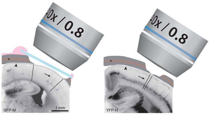
Schematic view of experimental preparations for in vivo imaging. In the chronic cranial window preparation (left), a piece of the cranial bone (dark gray) is removed (craniotomy) and replaced by a thin cover glass (blue). The dura (grey, arrowhead) remains intact. The exterior is sealed off from the brain surface by dental cement (pink). The craniotomy covers a large surface area (∼3 mm² in this example; area between dashed lines), which allows imaging of single cells with sparse labeling in the cerebral cortex (GFP-M line in this example, apical dendrite of layer 5 B (L5B) pyramidal cell indicated by arrow). For a thinned skull preparation (right) the cranial bone is usually thinned over a smaller area. The area that becomes transparent for imaging is in the order of 0.15 mm² (area between dashed lines). This technique is often used for mice with a higher labeling density (YFP-H line in this example). It should be noted that in both preparations the vascular plexus in the trabecular section of the cranial bone (asterisk) is damaged. Imaging is typically performed using ×20, ×40 or ×60 ‘long-working-distance’ water immersion ‘dipping’ objectives with numerical apertures varying from 0.8–0.95. All experiments using animals were carried out under institutional and national guidelines.

Technical considerations

Preparations

About two different surgical preparations have been used for long-term high-resolution imaging in vivo: chronic cranial windows and thinned skull preparations. With the chronic cranial window, a bone flap is removed (while leaving the dura mater unperturbed) and replaced by a coverglass in a single surgical session (Fig. 1 left panel; e.g., refs. 7,17). The imaging window provides an excellent optical access, allowing repeated high-resolution imaging with essentially unlimited time points and at arbitrary imaging intervals (Figs. 2–4). The size of the craniotomy ranges from ∼0.8 to 12 mm². This large field of view permits imaging of mice with very sparse labeling (e.g., GFP-M line^5,7; Fig. 1 left panel; see below). The chronic cranial window preparation is also suitable for larger animals, including rats and primates, in which the dura is opaque and thus has to be removed for imaging^3,31 and for neonatal mice, in which the skull is too fragile for thinning⁹. It can be combined with intrinsic optical-signal imaging (e.g., refs. 13^,20,21), injections of viral vectors^30,31, and implantation of electrodes, probes or other devices. In addition, miniature microscopes for freely behaving mice^35,36 and small diodes for photoactivation³⁷ are best used in combination with this type of preparation.

Figure 2.

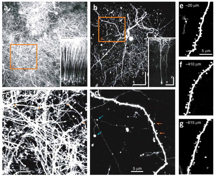
In vivo images of pyramidal neurons in the somatosensory cortex of YFP-H and GFP-M transgenic mice. (a) Top view of L2/3, layer 5 B (L5B) and L6 pyramidal neurons in a YFP-H mouse (maximum intensity projection of 160 sections, 5 μm apart, spanning cortical layers 1–5). The inset shows the side view of the same image stack, and the orange box is seen in more detail in c. Individual neurons or dendrites cannot be distinguished. (b) Top view of two L5B pyramidal neurons in a GFP-M mouse (maximum intensity projection of 159 sections, 5 μm apart). The inset shows the side view of the same image stack, and the orange box is seen in more detail in d. Individual neurons and dendrites can clearly be distinguished. See also Supplementary Movie 1. (c) Image of the apical dendritic tufts from the orange box in a (maximum value projection of 12 sections, 1.5 μm apart). Only a few short dendritic regions, likely from different pyramidal cells, are isolated and suitable for analysis of dendritic spines (in between asterisks). (d) Image of an apical dendrite from the orange box in b (maximum intensity projection of 12 sections, 1.5 μm apart). Small synaptic structures, such as axonal boutons (blue arrows) and dendritic spines (orange arrows) can be clearly distinguished. (e–g) Images of dendritic branches in the GFP-M line at different depths in the cortex (best projections of stacks of 4–7 sections, 1.5 μm apart). All images were acquired through a chronic cranial window, with equal excitation intensities (adjusted for increasing depth). Scale bars in a and b represent 10 μm (100 μm for insets). Images were obtained by RM and CP-C. All experiments using animals were carried out under institutional and national guidelines.

Figure 4.

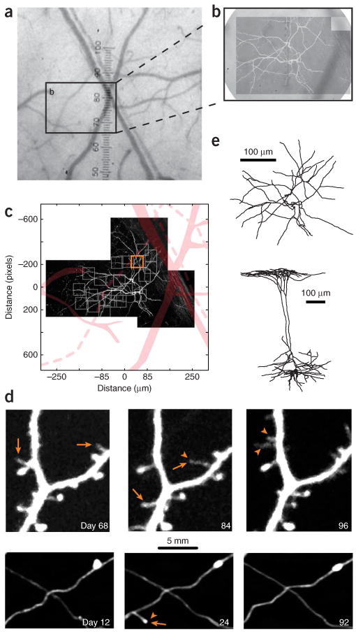
Long-term imaging of GFP-expressing pyramidal neurons in the adult neocortex. (a) Bright field image of the surface vasculature, as seen through a chronic cranial window. (b) Higher magnification of the imaged region. Superposed is the fluorescence image of the dendritic tuft of a layer 5 B (L5B) pyramidal cell. (c) The vasculature (displayed in pink) is used to register regions of interest of the dendrite (gray boxes). (d) Time lapse images of a dendritic (upper series) and axonal (lower series) segment, taken from a region of interest in c (orange box). Imaging was started 15 d after the surgery. Time stamps represent days after the first imaging session. Examples of appearing (arrowheads) and disappearing (arrows) spines and axonal boutons are indicated. (e) The entire neuron (imaged in c) has been reconstructed from in vivo images and the perfusion fixed brain. Top view of the apical tuft (above) and side view (below). Images obtained by AH, LW and GK. All experiments using animals were carried out under institutional and national guidelines.

The cranial window remains clear for several weeks to months, until regrowth of skull from the edges of the cranium, and thickening of the dura begins to degrade the image quality and ultimately terminates the experiment^7,9,15–17. As the preparation is sealed off by glass and dental cement, it is challenging to re-open the cranium (see PROCEDURE). The chronic cranial window technique is highly operator-dependent, with success rates in the order of ∼30–80%. Although the long-term optical clarity of the window depends on the quality of the surgery, the outcomes are sometimes unpredictable.

The thinned skull preparation leaves a thin (∼20 μm thick), optically clear layer of bone in place (Fig. 1 right panel; e.g., refs. 8,25). As the remaining bone is devoid of vasculature it thickens and becomes inflamed and opaque within 1 d after the surgery. Thinning, therefore, needs to be repeated before every imaging session. This can result in variations in imaging quality between sessions. In addition, because of the increasing opacity after repeated thinning, the experiment must often be terminated after the second or third session. However, the procedure can be carried out at any given time, and therefore the first and last imaging time point can be separated by long intervals, including months or, theoretically, even years. Skull thinning is usually carried out over a small area (∼0.1–0.3 mm²), as the shaving of larger parts of thin, unstable sheets of bone may contuse the underlying cortex (see ref. 25 and Supplementary Methods 1 online for a detailed description of the thinning procedure). This technique has therefore been used mainly on mice with dense and very bright labeling (e.g., YFP-H line^5,8; Fig. 1 right panel; see below).

Imaging in mice expressing fluorescent proteins

Transgenic mouse lines that express XFPs in sub-populations of neurons^5,6 (Fig. 2) have become an important tool for high-resolution imaging in vivo. Often, the XFP expression patterns are stable and sparse, thereby permitting imaging of isolated neuronal structures with high signal to noise ratios over long periods of time. The most popular lines include GFP-M (e.g., refs. 5^,7; Fig. 2b), mGFP-L15 (refs. 6,16), mGFP-L21 (refs. 6,9), YFP-H (e.g., refs. 5^,8,28,38; Fig. 2a), YFP-G^5,13 and GFP-S^5,15. A chronic cranial window provides a large field of view, allowing imaging in mouse lines with sparse expression patterns (such as GFP-M and mGFP-L15 and L21; Figs. 2b,d and 4c). As large parts of the dendritic and axonal arbor can be imaged, the identity of the parent cell can often be determined, either in vivo or by postmortem reconstruction (Figs. 4c,e)^{7,9,14–17,22}. Imaging sparsely labeled cells also allows extensive sampling of individual cells (Figs. 2d–g), and thus detection of neuronal (sub)type- and region-dependent effects^15,16,19,34. When combined with electrophysiological measurements⁷, intrinsic signal imaging^20,21,32,39, or post hoc anatomy^7,19, it allows for precise correlations between functional and structural plasticity. Although large data sets can be collected from mice with densely labeled neurons, such as the YFP-H line, it has not been possible to identify the neuronal subtype of the imaged dendrites and axons (Figs. 2a and 2c). Therefore, in these mice imaging is usually performed at the population level, mixing data from diverse cell-types^8,28,38,40. Furthermore, detection of all spines and/or boutons is challenging because of the high density of processes and the resulting background fluorescence. In addition, long-term expression of high XFP levels might have toxic effects, as has been shown for the YFP-H line⁴¹.

Direct gene delivery to brain tissue can be performed using electroporation and viral vectors. For example, in utero electroporation in mouse embryos has been used to label large groups of neurons in neocortex^42,43. Recombinant and replication-defective viral vectors, such as Lenti- and AAV based constructs, can be injected directly into the postnatal or adult mouse cortex and combined with long-term imaging. Depending on the injection volume, DNA concentration, vector backbone and promoter sequences, high expression levels of fluorescent proteins can be achieved in a relatively sparse population of neurons, permitting in vivo imaging^{4,29–31,37,39,44}.

Microscopy

Fluorescent neurons can be imaged in vivo using 2PLSM. The authors' laboratories typically use custom-built microscopes with detectors that are placed as close as possible to the objective, to increase the detection efficiency^45,46. A tunable Ti:sapphire laser is typically used as a light source. The wavelength of the excitation light depends on the fluorophore, but typically the cross sections of intrinsically fluorescent proteins are relatively broad (e.g., EGFP can be excited with reasonable efficiencies from 830 nm to 1,020 nm). High NA (×0.8–0.9, ×20–60) water immersion objectives are well suited for imaging of small structures, such as dendritic spines and axonal boutons. Sensitive photomultiplier tubes with high quantum efficiencies and low dark currents (e.g., Hamamatsu R3896 or H7422P) are adequate for detection of recurrent fluorescence.

Image analysis

The appearance or disappearance of dendritic spines and terminaux boutons should be scored on the basis of consistent, preset criteria (Fig. 5). As en passant boutons are continuous with the axon shaft, and smaller boutons are difficult to distinguish from nonsynaptic swellings⁴⁷, their appearance or disappearance can only be assessed by changes in brightness using threshold intensity-ratio measurements (see ref. 16 for details; Fig. 5l). To consistently score appearances and disappearances of spine and terminaux boutons, one has to use similar lookup tables at each time point. As small movements of the tissue (e.g., because of pulsation of nearby arterioles) can shift images in different sections, images need to be analyzed in three dimensions rather than in projections. Owing to the limited numerical apertures of long working distance water immersion objectives, and spherical aberrations in the brain, the spatial resolution along the axial dimension is poor relative to the sizes of typical synaptic structures. Therefore, small protrusions cannot always be detected or resolved if they emanate from the dendritic shaft perpendicular to the focal plane. We usually only include protrusions that emanate laterally from the dendritic shaft and if their lengths span more than 1 resolution unit (∼0.4 μm, typically 5 pixels; Fig. 5a), which exceeds the width of the haze of fluorescence around the dendrite. It is also important to verify that the intensity of the dimmest protrusion exceeds the noise in the images. The noise can be estimated by the standard deviation of the background fluorescence. We only include images for analysis if the fluorescence intensity of the (neck of the) dimmest protrusion is ∼5 times higher than the standard deviation of the background around the dendrite. In images with many fluorescent structures (axons and dendrites crossing each other), dim filopodia-like dendritic protrusions are often lost in the noise, and in addition can become indistinguishable from thin axons in the vicinity of dendrites. Furthermore, to compare spines over several imaging sessions one has to keep the fluorescence levels constant across images. All these criteria can considerably influence quantification of structural plasticity, and therefore contribute to differences in results reported in different studies from different labs (Fig. 6).

Figure 5.

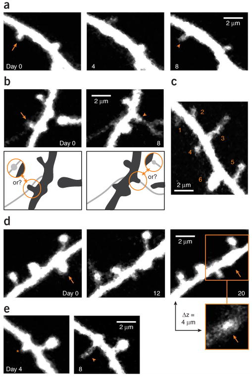
Examples of spine and bouton scoring criteria. (a) Examples of spines that are typically included in the scoring. The threshold is set at 0.4 μm (typically 5 pixels), which corresponds to lengths that span more than 1 resolution unit. (b) Protrusions that do not reach the threshold are ignored, even if they stand out clear from the haze of the dendrite. (c–e) Only laterally emanating protrusions are scored. The dendritic thickening in c can be resolved as a spine in the z axis of the image stack (d and e). However, it should not be included in the analysis, as this can only be done for very big spines (see also Fig. 6d). (f–i) Time lapse images (time = t₁–t₃). The spine in g is smaller and longer than the spine in f, but the position of its neck (x) and head (x₁) are similar to those of the spine in f. It is therefore to be scored continuously as spine 1. The spine in h is similarly shaped as the spine in f and g; however, the position of its neck (x') differs more than 0.5 μm from the original position (x). It can be scored as a new spine (depending on a preset threshold for x – x'). The neck of the spine in i has the same position as the spine in f and g. However, the position of its head (x₁';) differs more than 0.5 μm from the original position (x₁), and can thus be scored as a new spine (depending on preset threshold for x₁–x₁';). (j) Terminaux boutons (TBs) scoring thresholds. TBs are scored when their lengths span more than 1 μm and less than 5 μm. In order for a TB to be scored as a loss in time series, its length has to fall below a threshold of 0.4 μm (not shown). (k) Boutons that are located on stalks longer than 5 μm are scored as part of terminal branches. (l) En passant boutons (EPBs) are analyzed based on their intensity relative to the axon shaft. An axonal varicosity has to be three times brighter than the shaft to be scored as an EPB (see ref. 16 for more details). All experiments using animals were carried out under institutional and national guidelines.

Figure 6.

Examples of dendritic spines that have been inconsistently scored by different observers. (a) Example of a spine that has disappeared on day 4 (arrow) and re-appears on day 8 (arrowhead) at the same location. This can be scored as a loss and subsequent gain of a spine, but could also be interpreted as a failure to detect a persistent spine on day 4. (b) Examples of confusion between thin spines and axons. Arrow and arrowhead point to spines that are potentially lost and gained, respectively. However, the fluorescence could also represent boutons that are associated with the axon that crosses the dendrite and possibly has extended between day 0 and 8 (see schematic). (c) Spines of various sizes. The smallest spine (#1) is barely brighter than the background (×1.7) and has a signal-to-noise ratio (SNR) of ∼10. Spines 2–6 are increasingly brighter and will be detected with less ambiguity (e.g., spine 6: ×26 brighter than the background with a SNR of ∼160). (d) Example of a stubby spine (arrow) that emanates from the dendrite, both laterally and perpendicular to the image plane. Its lateral projection is less pronounced on day 20, but its head is still visible in a section, 4 μm above the center of the dendritic shaft. This spine therefore still emanates perpendicular to the plane of imaging on day 20. (e) A new protrusion (arrowhead) extends from a stubby spine or thick nodal part of the dendritic shaft (asterisk). A first criterion should determine whether the thickening represents a spine or not, and a second criterion is needed to decide whether the extending protrusion represents a new spine. Time stamps represent days after the first imaging session in all examples. Images obtained by A.H. and L.W. All experiments using animals were carried out under institutional and national guidelines.

In general, we feel that measurements of absolute numbers of turnover of small synaptic structures are subject to significant systematic differences between different observers (perhaps as large as a factor of two; see ANTICIPATED RESULTS) and should therefore be treated with caution. On the other hand, the scoring of changes in structural plasticity, e.g., before and after sensory deprivation^7,19–21,32, is more robust if turnover is scored in a blind manner using consistent criteria. In addition, post hoc analysis by super-resolution reconstruction of the imaged structures (e.g., retrospective serial section EM²², see also ref. 48) can be performed to verify scoring criteria.

The appearance and disappearance of small structures can be expressed by the survival function (SF) and the turnover ratio (TOR). The survival function describes the fraction of structures that remain present over time; SF(t) = N(t)/N₀, where N₀ is the number of structures at t = 0, and N(t) is the number of structures of the original set surviving after time t. By definition SF(0) = 1. The TOR describes the fraction of structures that appear and disappear from one time point to the next TOR (t₁, t₂) = (N_gained + N_lost)/(N(t₁) + N(t₂)), where N(t₁) and N(t₂) are the total number of structures at the first and second time point, respectively. If the number of appearances and disappearances are similar, TOR (t₁, t₂) = (N_gained + N_lost)/(2xN(t₁)) and [1−SF(t₂−t₁)] ≈TOR (t₁, t₂).

Controls

To control for the detection sensitivity of the preparation, the results from the in vivo imaging can be compared with images from fixed brains (naive or experimental mice). Spine and bouton density and the distribution of their sizes should be comparable under all conditions^16,17. To control for the stability of the preparation image series taken shortly after surgery can be compared with image series taken several weeks later. Any surgical procedure (craniotomy and skull thinning alike) carries the potential risk of acute and transient effects on the brain due to mechanical stress and prolonged anesthesia. Thus, data collection immediately after the surgery should be avoided unless the experimental design demands this. To illustrate such control experiments, we provide examples from several of our laboratories, in which spine and bouton densities and their turnover were measured with different intervals from day 1 until several weeks after the surgery^20,21,34 (see ANTICIPATED RESULTS; Figs. 7 and 8). Similarly, the ultrastructure and glial cell reactivity can be estimated at several time points after the surgery by EM and immunohistochemical detection of glial cell markers, respectively^7,25,34 (see ANTICIPATED RESULTS; Figs. 9 and 10).

Figure 7.

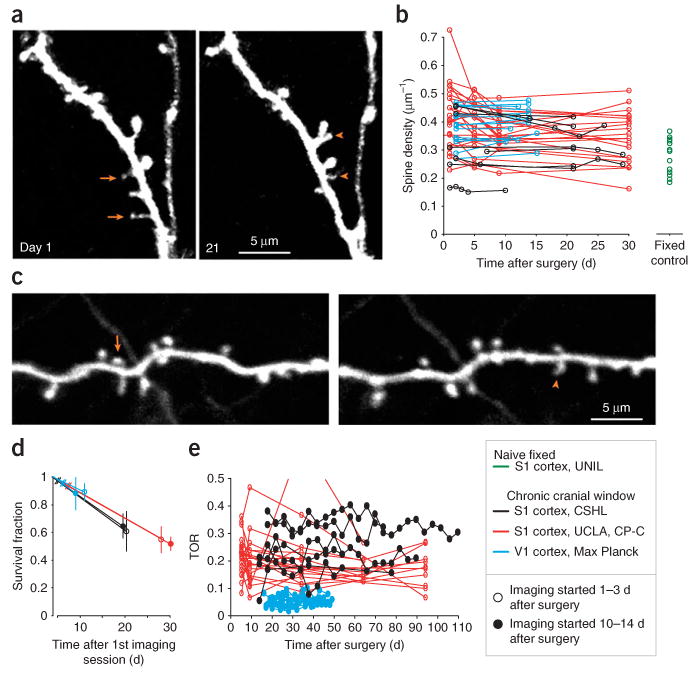
Quantification of layer 5 B (L5B) pyramidal cell dendritic spine density and turnover. (a) Example of spines in somatosensory cortex, imaged through a chronic cranial window 1 d after surgery and 20 d later. Examples of some spines that have disappeared (arrows) and appeared (arrowheads) over this period are indicated. (b) Spine densities vary from cell to cell under the cranial window (black (data from A.H., V.D.P., K.S., L.W.), red (data from R.M., C.P.-C.) and blue (data from T.B., S.B.H., M.H., T.K., T.D.M.-F.)) as well as in the naive cortex (green (data from A.H., J.C., G.K.)), and remain relatively stable on an average over several weeks of imaging. (c) Example of spines that have disappeared (arrows) and appeared (arrowheads) in visual cortex, imaged through a chronic cranial window 2 d after surgery and 12 d later. (d) Average survival fractions of spines. Open markers represent survival fractions in experiments where imaging was started immediately after the surgery, solid markers represent experiments that included a waiting period of 2 weeks after the surgery (black points represent data from earlier studies¹⁹). (e) Turnover ratio (TOR) over 4 d imaging intervals. Imaging was started immediately after the surgery (red, same mice as in b) or after a 2-week waiting period (black and blue, data from different studies). TORs are, on an average, constant over extended periods of time (> 90 d). All experiments using animals were carried out under institutional and national guidelines.

Figure 8.

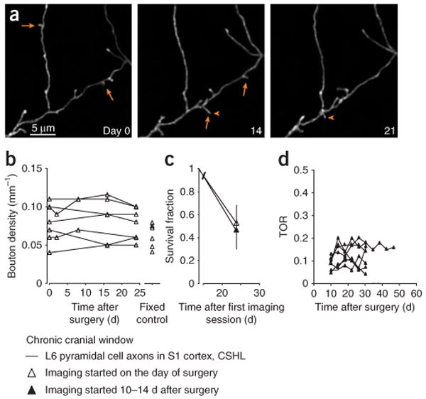
Quantification of L6 terminaux bouton density and turnover. (a) Examples of appearing (arrowheads) and disappearing (arrows) terminaux boutons in the somatosensory cortex, imaged through a chronic cranial window on the day of the surgery, and 14 and 21 d later. (b) Bouton density under the cranial window remains constant over time and is comparable with bouton densities in naive fixed brains (fixed control). (c) Survival fractions of boutons imaged immediately after the surgery are similar to those imaged after a recovery period of 10–14 d. Open markers represent survival fractions in experiments, where imaging was started immediately after the surgery (same mice as in b), solid markers represent experiments that included a waiting period of 2 weeks after the surgery (results from an earlier study¹⁶). (d) Turnover ratio (TOR) over 4-day imaging intervals. Imaging was started ∼10 d after the surgery (data from different studies). TORs are, on average, constant over long periods of imaging (> 45 d). Data by V.D.P. All experiments using animals were carried out under institutional and national guidelines.

Figure 9.

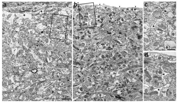
Qualitative assessment of the ultrastructure under a chronic cranial window. Electron micrographs showing the upper region of L1 in the primary somatosensory cortex in a control (a) and an operated (b) mouse 15 d after surgery. The image in b is taken at the position below the center of the cranial window. The basal lamina is indicated (arrowheads) in each image and below this are astrocytic profiles (stars). Both images show the tightly packed arrangement of axons and dendrites in this upper region of cortical layer with no clear differences in the amount of glia or neurons present. Boxed areas (c and d) show typical astrocytic profiles that can be found in the vicinity of synapses (stars) between axonal boutons (b) and dendritic spines (sp). Data obtained by G.K. and J.C. All experiments using animals were carried out under institutional and national guidelines.

Figure 10.

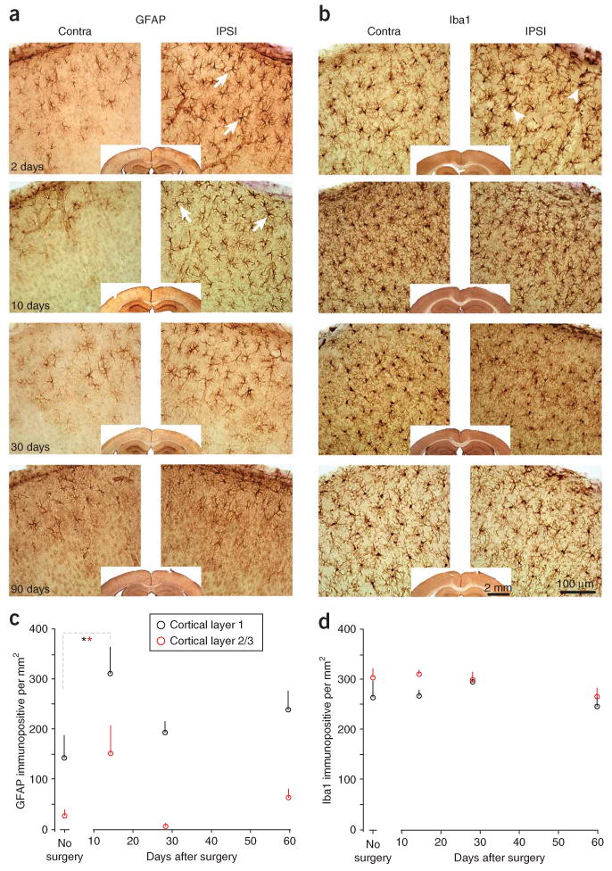
Immunohistochemical staining of glial markers under a chronic cranial window. (a) Immunostaining for the astrocyte marker GFAP, at several time points after surgery (time stamp in left lower corners). Operated hemisphere is displayed on the right, control hemisphere on the left. A transient and mild enhanced immunostaining is observed at 2 d and 10 d (GFAP) after surgery. The enhanced immunoreactivity is partly caused by an increase in the number of moderately GFAP-immunopositive astrocytes in the L1 and 2/3, as well as by an increase of GFAP levels in some cells (e.g., arrows). (b) Alternating sections of the same mice as in a, stained for Iba1, a microglia marker. Some microglial profiles are slightly thicker on day 2 after the surgery (arrowheads), but remain essentially unchanged over the course of the experiment. (c,d) Quantification of GFAP (c) and Iba1 (d) immunopositive cells in L1 (black) and L2/3 (red) from a different experiment in a different lab. The number of GFAP immunopositive cells is significantly (*P < 0.05, ANOVA) increased during the first 2 weeks after surgery, but return to control levels afterwards. Iba1 immunoreactivity remains unchanged. Data in a and b were obtained by R.M. and C.P.-C. Data in c and d were obtained by W.-C.A.L. and E.N. Qualitatively all labs observed phenomena that were comparable to the examples presented in this figure. All experiments using animals were carried out under institutional and national guidelines.

Applications of the chronic cranial-window preparation and outlook

Chronic cranial windows have been used by several research groups to image the structure of cortical neurons over periods of weeks–months^{4,7,9,13–17,19–21,28,29,31,32,34,38}. A variety of the following parameters have been measured: dendritic and axonal growth or stability^{7,9,13–16,29,31,34}; dendritic spine and axonal bouton turnover^{7,16,17,19–21,28,32,38}; dendritic spine, axonal bouton volume changes^16,19,21 and dynamics of GFP-tagged synaptic proteins^4,39. Imaged neurons are easily identified in vivo and recovered in the postmortem material^7,15,19, axons can be traced back to their cell body^9,16 and neuronal structures can even be reconstructed with serial-section electron microscopy^7,16,22,48. The lengths and complexities of dendritic and axonal arbors, as well as their spine and bouton densities, remain stable for months after the surgery^{7,13–17,19,34}. Similarly, baseline structural dynamics of synaptic structures remain constant^{7,13,15–17,19}. The brain underlying chronic cranial windows display only minor and transient changes in the expression of glial-cell markers during the first 2 weeks after the surgery^32,34.

The ability to image and reconstruct entire neuronal structures in sparsely labeled transgenic XFP mice over arbitrary and unlimited imaging time points for several months represent a distinct advantage of the chronic cranial window. The chronic cranial window is therefore exquisitely suitable for studies aiming at a detailed investigation of the relationship between structural dynamics and functionality of neuronal networks.

Materials

• Ketamine (Ketaset, Wyeth, 100 mg ml⁻¹)

• Xylazine (Rompun, Bayer Healthcare, 20 mg ml⁻¹)

• 2,2,2-Tribromoethanol (Sigma-Aldrich, cat. no. T48402)

• 2-methyl-2-butanol (Sigma-Aldrich, cat. no. 240486)

• Isoflurane (Forane, Baxter, 100%)

• Bottled oxygen (O₂, 100%)

• Dexamethasone (dexamethasone sodium phosphate injection 4 mg ml⁻¹, equivalent to 3 mg ml⁻¹ dexamethasone, Mephamesone, Mepha Pharma)

• Xylocaine liquid (Lidocaine 1% + epinephrine 1:100,000 solution, Astrazeneca)

• Carprofen (Rimadyl, Pfizer, 50 mg ml⁻¹)

• Buprenorphine (Temgesic or Buprenex, Webster Veterinary, cat. no. 07-836-8775, 0.3 mg ml⁻¹)

• Enrofloxacin (Baytril, Bayer Healthcare, cat. no. 08713254, 22.7 mg ml⁻¹)

• Sulfamethoxazole (Gantanol, Hi-Tech Pharmacal, cat. no. NDC50883-823-16, 500 mg per tablet)

• Trimethoprim (Trimpex, Roche, 200 mg per tablet)

• NaCl (Sigma, cat. no. S9888)

• KCl (Sigma, cat. no. P9333)

• Glucose (Sigma, cat. no. G5767)

• HEPES (Sigma, cat. no. H8651)

• CaCl₂ (Sigma, cat. no. C1016)

• MgSO₄ (Sigma, cat. no. M2643)

• Sterile lubricant eye ointment (Stye, Del Pharmaceuticals, cat. no. MME-72571) or Optical gel (Nye Optical, cat. no. OC431A-LVP)

• Sterile saline (VWR International, cat. no. 101320-570)

• 70% Ethanol or isopropanol (Sigma, cat. no. I9516)

• Lactated ringers solution (Baxter Healthcare, cat. no. 2B2324X)

• Sterile Gelfoam sponges (Pfizer, cat no. 9035301) or Davol Avitene Ultrafoam (Bard Inc., cat. no. 1050050)

• Agarose (Sigma, cat. no. A9793)

• Glue VetBond (3M, cat. no. 1469SB) or Krazyglue (Krazy Glue, cat. no. KG585)

• Dental acrylic (Jet repair, Lang Dental, cat. no. 1234) or bone cement (Palacos R, Biomet, cat. no. 424800)

• Mice expressing fluorescent proteins in the cerebral cortex. Identical procedures can be used to image neurons or vasculature labeled with synthetic fluorescent molecules, or to image intrinsic optical signals

  : All experiments using animals should be carried out under institutional and national guidelines.

Equipment

• Water-recirculation heating blanket for mouse (Gaymar, e.g., cat. no. TP3E)

• Hot glass-bead sterilizer (Fine Science Tools, cat. no. 18000-45)

• Stereotaxic frame (Stoelting, cat. no. 51600)

• A high speed air driven dental drill (Midwest Tradition, e.g., cat. no. 790044) with $\frac{1}{4}$ FG dental drill bits (Dental burrs, Henry Schein, cat. no. 100-7205). Alternatively, a high speed micro drill (Fine Science Tools, cat. no. 18000-17) with 0.5 mm round steel burrs (Fine Science Tools, cat. no. 19007-05)

• Dissecting microscope (Stemi 2000, Zeiss)

• Inhalational anesthesia vaporizer (Harvard Apparatus, cat. no. 728125)

• Forceps, blunt and sharp; scissors

• Cotton-swab applicators (low-lint types, Puritan, cat. no. 896-WC).

• Glass coverslips (1 thickness, from Electron Microscopy Science, cat. no. 72195-05 or Bellco Glass, cat. no. 1943-00005)

• Titanium or stainless steel bars (custom made) or any other device to attach the mouse head to the microscope stage

• In vivo 2PLSM microscope, ×40, 0.8 NA water immersion objective or similar

• Image acquisition software: e.g., ScanImage⁴⁹ custom written in MatLab (Mathworks); or software integrated in commercial 2PLSM setups

Reagent Setup

Ketamine/Xylazine mixture

Mix 13 mg ml⁻¹ of ketamine and 1 mg ml⁻¹ of xylazine in distilled, sterile H₂O. This mixture can be made in advance and stored in the dark at room temperature for few weeks.

Tribromoethanol (Avertin, 12.5 mg ml⁻¹)

Dissolve 2.5 g of 2,2,2–tribromoethanol in 5 ml 2-methyl-2-butanol, heat to 40 °C and stir. Add distilled, sterile H₂O to a final volume of 200 ml. This mixture can be made in advance and stored in the dark at 4 °C for 2 weeks.

Sterile cortex buffer

Dissolve 125 mM NaCl (7.21 g NaCl), 5 mM KCl (0.372 g KCl), 10 mM glucose (1.802 g glucose), 10 mM HEPES (2.38 g HEPES), 2 mM CaCl₂ (2 ml 1M CaCl₂) and 2 mM MgSO₄ (2 ml 1M MgSO₄) in distilled H₂O (1 l of dH₂O). The buffer should be maintained at pH 7.4. Sterilize the solution by passing it through a sterilization filter. The solution can be prepared in advance, aliquotted and stored at 4 °C for at least a month.

1.2% Agarose

Warm 0.3 g of agarose in 25 ml of cortex buffer until fully dissolved. This solution must be freshly prepared and sterile for each experiment, and kept hot. It must be stirred frequently during the procedure. Before applying the hot agarose to the cortex, allow it to cool briefly and check that the temperature is not above ∼37 °C.

Procedure

Surgery 1 h

• 1|Anesthetize the mouse with an intraperitoneal (i.p.) injection of ketamine (0.10 mg g⁻¹ body weight) and xylazine (0.01 mg g⁻¹ body weight) mixture. Alternatively, 1.25% avertin (i.p., 0.02 ml g⁻¹ body weight) or isoflurane (4% for induction; 1.5–2% for surgery with ∼0.5 liter min⁻¹ O₂; especially for young mice less than 4 weeks old) can be used; note that we have experienced a higher susceptibility to dural bleeding during surgeries under isoflurane anesthesia. Shave the animal's head.

  All experiments using animals should be carried out under institutional and national guidelines.

• 2|Place the mouse on the heating blanket and stabilize the head in a stereotaxic frame. Protect the eyes from dehydration and irritation by applying vaseline and/or an eye-ointment.
• 3|Administer dexamethasone sodium phosphate (0.02 ml at 4 mg ml⁻¹; ∼2 μg g⁻¹ dexamethasone) by an intramuscular injection to the quadriceps. Dexamethasone reduces the cortical stress response during the surgery and prevents cerebral edema.

  Preventing cerebral edema during the surgery is critical for successful surgeries. In addition, inflammation can be reduced by treatment with carprofen (daily i.p. injections of 0.3 ml from a 0.50 mg ml⁻¹ stock), starting immediately before the surgery.

• 4|Wash the scalp with three alternating swabs of 70% ethanol (or 70% isopropanol) and betadine. Using scissors, remove a flap of skin, ∼1 cm², covering the skull of both hemispheres (Fig. 3a).

  Use clean and sterile surgical tools. They can be autoclaved or sterilized with a hot glass-bead sterilizer.

  Do not apply ethanol, betadine or isopropanol to open wounds or exposed skull.

• 5|Apply 1% Xylocaine to the periosteum of the skull and the exposed muscles at the lateral and caudal sides of the wound (arrows in Fig. 3a). Remove the periosteum by gently scraping the skull with a scalpel blade. This will help the glue to adhere to the bone. To minimize bleeding of the skin and skull, epinephrine can be administered (optional, 1 small drop of lidocaine (1%) + epinephrine (1:100,000) solution directly onto the skull). Next, gently scrape the periosteum away from the bone with a blunt spatula, avoiding bleeding. If needed, depending on location of cranial window, separate the temporalis muscle.

  

• 6|Mark the cortical area of interest with a pen or draw it gently with the dental drill (e.g., young adult barrel cortex: interaural−1.5 mm from bregma, 3.5–4 mm lateral; adult visual cortex: interaural 1.7 mm rostral from lambdoid suture, 1–5 mm lateral; be aware that coordinates vary considerably with age).
• 7|Apply a thin layer of cyanoacrylate (vetbond or krazyglue) to the nearly dry skull, the temporalis muscle and wound margins to prevent the seepage of serosanguinous fluid, but spare the area of trepanation. The layer of cyanoacrylate provides a better base for the dental acrylic to adhere to. Apply a thin layer of dental acrylic on top of the glue after it has dried (Fig. 3b), again making sure not to apply any on the area of interest. This step can also be performed after Step 8.
• 8|Begin thinning a circular groove in the skull around the region of interest. Drill slowly ( $\frac{1}{4}″$ drill bit) and apply saline or cortex buffer regularly to avoid heating, which can bruise the dura. Leave an island of skull (diameter ∼2–4 mm) intact in the center. The cortical surface vasculature should become visible under the circular groove (especially when damp with buffer). Expect to encounter some bleeding from the skull owing to tearing of the vascular plexus in the trabecular section of the cranial bone.

  Care should be taken not to apply excessive pressure with the drill as this might puncture the skull and injure the dura. Check the thickness of the skull in the groove by gently pushing on the central island of the cranial bone with a fine probe (be careful not to press it down into the brain). If the island moves when lightly touched, it is ready to be removed. Drilling across bone sutures might cause excessive bleedings and should be avoided (be aware that when aiming for visual cortex this can often not be avoided, and one should wait for bleedings to stop until proceeding). Note that we have also experimented with cutting through the skull using a scalpel. This causes more initial bleeding from skull blood vessels, but has a lower risk of bruising the dura from overheating. However, we do not have enough data to provide information on the stability of such a preparation.

  

• 9|Next, gently insert the tip of sharp (angle-tipped) forceps into the trabecular (spongy) bone, which is exposed on the side of the groove. Keep the tip in a horizontal position and try to avoid direct perforation of the thinned bone with the forceps, which could cause injury of the dura. Slowly lift the central island of skull bone, exposing the dura (Fig. 3c).

  The successful removal of the skull is achieved best when carried out under a large drop of cortex buffer; as one edge of the skull is lifted with the forceps the fluid helps the flap of skull to detach from the dura. Best results are obtained when the skull island is gently tugged laterally (wiggling it back and forth) until the thinned bone tears at the bottom of the groove. Once the bone flap is completely loose, lift it out of the cortex buffer.

• 10|Under ideal circumstances the dura should not bleed (Fig. 3c). However, as the dura is attached to the inner table of the cranium, some superficial capillaries might tear during removal of the cranial bone. Small focal bleeding typically disappears spontaneously or can be controlled by applying Gelfoam. Gelfoam or Davol avitene ultrafoam should be cut into ∼7 mm² blocks and soaked in cortex buffer before use. Wet Gelfoam can be applied directly onto the dura. Again, no pressure should be applied to the brain. At this point, only Gelfoam (or something similar) can be applied on the dura to stop the bleeding or to keep it wet. Cotton swabs or tissue paper are completely discouraged.

  

• 11|Complete the optical window by covering the unblemished dura with a circular coverglass (3–7 mm diameter, #1 thickness), flush with the skull (Fig. 3d). The dura should still be wet at this point, but the skull around it needs to be dry. The glass coverslip should be at least as wide as the craniotomy and it should be as close to the brain as possible (∼100 μm). The glass can be directly applied, or alternatively the dura can first be covered with a very thin layer of melted 1.2% agarose. The agarose may help to minimize movement because of pulsations of blood vessels. Agarose is particularly useful in young mice because there is more space between the skull and the underlying brain. Apply the melted agarose when it has nearly solidified (close to body temperature). Gently push it down with the coverslip and let the excess agarose float away from under the glass. The agarose should seal the brain from the air and the dental cement that is applied later. Once the agarose has solidified, excess amounts can be trimmed carefully from the edges of the window using a scalpel. The surface of the skull should be dried again. If agarose is omitted, apply a small amount of cyanoacrylate all around the coverslip and let it dry. Be careful to avoid letting any glue or cement contact the dura, as it will not remain transparent.

  Make sure the glass is as close to the dura as possible (ideally within ∼100 μm). If the glass is farther off, the opacity of the intermediate fluid and/or agarose will degrade the image quality.

  

• 12|Seal the optical window to the skull with dental cement, covering all the exposed skull, wound margins and cover glass edges (Figs. 3e,f). A clean, small titanium or stainless steel bar with tapped screw holes can be embedded into the acrylic over the intact hemisphere to stabilize the animal for subsequent imaging sessions (Fig. 3f). The screw threads are kept clear of acrylic. It is necessary to allow the acrylic to set before manipulating the mouse or bar (typically 30 min is sufficient). The bar should be level with the glass surface to position the window horizontally under the microscope and perpendicular to the optical axis of the microscope.

  

• 13|Acute experiments can be done for the duration of the anesthesia (typically up to 1 h after surgery for ketamine/xylazine or avertin, or for several hours under isoflurane anesthesia).
• 14|For chronic experiments, lactated ringers solution (i.p. or s.c., 0.015 ml g⁻¹ body weight; saline is also sufficient) and the antibiotic enrofloxacin (optional; s.c. 5 μg g⁻¹ body weight) may be administered at this point to prevent dehydration and infection, respectively. Allow the mouse to recover on the heating pad and returned to its cage for recovery under observation. Wet food can be given to facilitate chewing and hydration. To reduce pain, the opioid analgesic, buprenorphine (buprenex, s.c., 0.1 μg g⁻¹ body weight, twice daily) may be administered for 2–5 d. Allow the mouse to recover for an additional 7–10 d before imaging.

  Windows often clear and improve over this recovery time. Large cages with high ceilings can help to prevent the mice from detaching the head cap or damaging the window. It should be noted that the window-covered craniotomy can remain clear for months without additional treatments (Supplementary Fig. 1). However, anti-inflammatory drugs and antibiotics can be administered to prevent complications; sulfamethoxazole (1 mg ml⁻¹) and trimethoprim (0.2 mg ml⁻¹) can be chronically administered in the drinking water throughout the experiment. Carprofen can be administered daily by an i.p. or s.c. injection (see Step 3).

  

Figure 3.

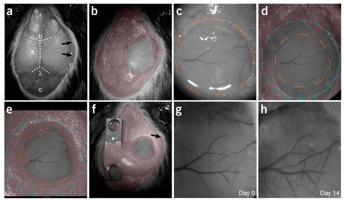
Chronic cranial window surgical procedure. (a) The skin and periosteum have been removed. The right temporalis muscle (arrows) has been separated from the bone. The cranial bone has been covered with a thin layer of cyanoacrylate (PROCEDURE Steps 5–7). Dashed lines indicate cranial sutures, bregma (b) and lambda (l). The skull is exposed from the cerebellum (c, caudal) to the olfactory bulb (r, rostral). (b) A thin layer of dental acrylic (pseudo colored in red) has been applied. The area of interest remains uncovered (PROCEDURE Step 7). (c) A circular groove has been drilled (dashed orange line), and the island of cranial bone has been removed. The brain remains covered with buffer. The superficial blood vessels become clearly visible (PROCEDURE Steps 8–10). (d) A circular cover glass (#1 thickness, blue dashed circle) is covering the brain and part of the skull (PROCEDURE Step 11). (e) Dental cement has been applied on top of the skull and part of the cover glass, sealing off the exterior (PROCEDURE Step 12). (f) All of the exposed skull, wound edges and the temporalis muscle (arrow) have been covered with dental cement, and a titanium bar (asterisk) with threaded holes has been attached. (g) Bright field view of the superficial blood vessels through the glass window immediately after the surgery (day 0). (h) The same preparation 14 d later. Note that the surface vasculature patterns remain unchanged, and the center of the window remains transparent. (The window can remain transparent for several months, see Supplementary Fig. 1.) Surgery in this example was performed by VDP. All experiments using animals were carried out under institutional and national guidelines.

Imaging 45 min

• 15|For imaging, anesthetize animals with ketamine/xylazine at ∼2/3 surgical dose, with 1.5% isoflurane or with 1.25% avertin (i.p., 0.015 ml g⁻¹ body weight). Place 1.5% agarose or optical gel around the edges of the imaging window, forming a small well for the water immersion objective (alternatively a permanent shallow well can be sculpted out of dental cement at time of the surgery). Place animals under the microscope, resting on a heating pad with their head immobilized, using either a stereotaxic frame or by attaching the bar on their head to a stable holder. To facilitate identical positioning in subsequent imaging sessions the bar should have a read-out for the rotation angle of the mouse's head. To minimize optical aberrations, make sure that the coverslip and dura are oriented perpendicular to the optical axis of the microscope.
• 16|In the first imaging session, search for suitably labeled neurons using equipment and set up as described in the experimental design. Make an inventory of good locations and store their coordinates relative to a fiducial point in the vascular pattern on the dura (Fig. 4a).

  Illumination of fluorescent structures (e.g., while searching for suitable areas) could cause photobleaching and phototoxicity, collectively called photodamage. To minimize photodamage the duration of light exposure should be kept as short as possible. To test for photodamage, revisit the structures imaged earlier at the end of the imaging session, and check for unexpected alterations in structures (e.g., blebbing and beading of dendrites and axons). The light exposure per imaging session can be reduced by blocking the laser light during the ‘flyback’ of the galvanometer mirrors using electro-optic modulators (Pockels cell). We do not consider this crucial for imaging XFPs with long sampling intervals. We estimate that for a chronic cranial window ∼25–100 mW of power (at 910 nm) in the back focal plane (of which 50% is usually transmitted by the microscope objective) is typically sufficient. Owing to scattering of photons only 10% of the power at the surface of the brain is delivered to the laser focus ∼100–150 μm deep⁴⁶, resulting in 1–5 mW at the focus. In contrast, ∼500 mW of near-infrared light in a stationary diffraction-limited spot heats aqueous medium by 1 °C (e.g., ref. 50). The excitation laser should therefore impose only a minimal thermal load on the brain.

  

• 17|Take several adjacent low magnification image stacks of the cell of interest and create an overview (off-line) of its dendritic or axonal arbor using maximum intensity projections. Use the low magnification overview as a guide to choose the regions of interest (ROIs), which will be imaged with high magnification (Figs. 4a,c). Take several adjacent high-magnification image stacks of as many different branches of dendrites or axons as possible. Try to follow dendrites all the way to the cell body to identify cell (sub)type and cortical layer of origin (Fig. 2b)^7,15,17. For axons it is critical to image long stretches. This will ultimately help in the identification of the axonal (sub)type and tracing in post fixed material (see refs. 9^,16 for details).
• 18|Store coordinates of every ROI relative to the vascular pattern on the dura or to fiducial points in low magnification images (Figs. 3g, 4a,c and Supplementary Fig. 1). Image the same ROIs over time. Image stacks typically consist of sections (e.g., 512 × 512 pixels; ∼0.08 μm per pixel) collected in 1 μm steps (3–5 samples per resolution element). In addition, low magnification images (e.g., 512 × 512 pixels; ∼0.3 μm per pixel; 3 μm steps) can be used for overview. Care should be taken to maintain close to identical fluorescence levels across imaging sessions by adjusting the excitation power.

  Verify that the smallest synaptic structures can be detected. Spines and boutons volumes can be smaller than 1 × 10⁻¹⁷ liters, corresponding to tens of GFP molecules (assuming ∼10 μM GFP concentration), which is close to the detection limit for in vivo 2PLSM. The spine and bouton densities measured from in vivo images should be identical to measurements in fixed tissue. We have used retrospective serial-section electron microscopy and established that with a chronic cranial window, even the smallest structures can be detected in the in vivo images^7,17,22. Simple ways to verify that all structures are detected include: (1) increasing the excitation power should not reveal additional spines; (2) the signal fluorescence intensities are significantly different from the noise (e.g., blurred haze arising from the large dendritic volume) by measuring the signal-to-noise ratio (SNR) of spines and boutons in the acquired images (Fig. 6c)^7,17.

  

Image analysis Depending largely on the number of images and time points, and type of analysis; from ∼1 h to several days per mouse

• 19|Analyze images with the appropriate software (e.g., ImageJ or custom software^7,15–17,20). Dendritic spine and axonal bouton structural plasticity can be measured by scoring complete appearances and disappearances.

  

  Steps 1–14: ∼1 h

  Steps 15–18: ∼45 min

  Step 19: Depending largely on the number of images and time points, and type of analysis; from ∼1 h to several days per mouse.

  

  Troubleshooting advice can be found in Table 1.

TABLE 1.

Troubleshooting table.

Problem	Possible reason	Solution
Step 5: Excessive muscle exposed (lateral or posterior)	Too much skin removed	Gently pull skin to cover muscle and glue onto skull with cyanoacrylate (vetbond)
Bleeding from muscles	Too much skin removed; muscles manipulated too roughly or with a sharp object	See above; use blunt object to gently push muscle aside
		Note: There should be no bleeding from the muscles, if bleeding occurs or continues this will destabilize the preparation and there is a risk the cranial window will come off
Step 8: Excessive bleeding from skull	Damaged blood vessel (skull vessels are normally disrupted during the drilling process)	Soak up blood with Gelfoam and allow blood to clot before applying agarose or dental cement
Drill pierces through skull and dura	Excessive pressure or speed applied with drill	Discard, as the dura has been compromised, which usually damages the underlying cortical tissue. In future preparations, avoid drilling at very high speeds and applying pressure.
Step 10: Brain swells and bulges through the craniotomy	Edema caused by general disruption during the surgical procedure; anesthesia too light	Peripheral administration of dexamethasone before surgical manipulations, keep the skull and the brain surface moist and cool during drilling, reduce pushing on the skull and excessive manipulations when cranium is opened. Reduce time with the dura exposed. Administer more anesthesia
After the island of cranial bone is removed the brain surface appears bruised	Subdural bleeding due to blood vessel damage (see above)	Discard, as the dura has been compromised, which usually damages the underlying cortical tissue. In future preparations, avoid drilling at high speeds
Step 11: Bleeding suddenly appears just before agarose or glass being applied	Dura may have over dried; dura has been touched	Apply wet Gelfoam and wait; keep dura moist at all times; if bleeding is subdural, discard the mouse
Air bubble in agarose	Air pocket leaked into agarose while it was being applied or trimmed around the craniotomy	Gently manipulate the edge of the agarose to allow the bubble to escape; apply more cortex buffer. If bubble persists, gently remove agarose and reapply fresh
Agarose does not set rapidly	Agarose concentration too low; agarose was too hot at time of application	Remove agarose and adjust concentration (1.2%– 1.5% is ideal); apply agarose again when it is close to body temperature and is just about to solidify
Agarose sets immediately and has opaque, brittle appearance	Agarose concentration is too high; agarose too cold at time of application	See above
Bleeding appears after agarose is applied	Blood vessels have been disrupted or dura dried too much prior to agarose being applied; agarose was too hot; buffer concentration not correct	See above. If bleeding is less, continue, the blood will usually disappear within the first week following surgery. If bleeding continues, the agarose can be very carefully removed and re-applied. This is usually a predictor that long-term quality of window will be poor
Coverglass sits too far off skull	Cranial bone is too thick (common in old adult mice)	Gently thin the surrounding skull to allow coverglass to sit as flush as possible with dura; use a cover glass that fits in the cranium
Step 12: Dental cement floods craniotomy	Insufficient agarose or buffer applied over craniotomy; cover glass was lifted during application of cement; cement was too liquid when applied	Discard, as the dura will be compromised
Step 14: Cranial window is not optically clear immediately after surgery	Coverglass is dirty	Clean coverglass with 70% ethanol before application
	Dura came into contact with cyanoacrylate adhesive or dental cement	Discard if dura was damaged or wait for clearance if opacity is because of agarose. Ensure cyanoacrylate and dental cement are kept away from the immediate craniotomy area
Coverglass breaks	Edges of coverglass were insufficiently covered with dental acrylic	Discard. In future preparations, ensure coverglass edges are sufficiently covered with dental acrylic
	Animal has damaged coverglass by bumping into cage rack	Use cages with high ceilings
Cranial window preparation becomes loose or falls off	Regrowth of tissue pushes the window off	Discard
	Insufficient application of vetbond and/or dental acrylic	In future preparations, ensure all wound edges and exposed skull are covered with dental acrylic
	Head cap got stuck in cage rack	Use cages with high ceilings
Milky substance appears under window in days following surgery	Infection	Discard. In future, ensure that all surgical instruments are sterilized before surgery, surgical area is clean and surgeries are performed quickly and efficiently. Keep coverglasses stored in 70% EtOH. Let them dry before applying onto the dura. Administer antibiotics
Step 16–18: Imaging is successful within the first few days following surgery, after this period no or only faint fluorescence can be detected	Inflammatory reaction	Try imaging again after 7–10 d, the window will normally settle and clear during this time Postsurgical treatment with carprofen, sulfamethoxazole + trimethoprim
Imaging is no longer possible in the weeks following surgery	Skull regrowth	Terminate experiment. A last time point can be obtained by gently removing the head cap and regrown cranial bone (is usually very thin). Expect more bleedings
		Neurons can also be relocated and imaged in the fixed whole mount brain for a last imaging session (fast and careful perfusion is essential to maintain structural integrity)
Sudden large amplitude motion artifact during imaging	Animal is starting to come out of anesthesia	Re-anaesthetize animal and ensure head and body are stabilized before recommencing imaging
	Head cap is lose	Reseal with dental cement and glue if not completely detached. If air has come under window, discard. Usually, this rescue attempt fails
	Animal gasps because high dose of isoflurane	Reduce the percentage of isoflurane
Continuous small amplitude motion artifact during imaging	Movement due to heart rate (neuronal process close to large caliber vessel) and/or breathing	This cannot always be avoided. However, if the excessive movement is because the ROI is situated near a large vessel, select another ROI. For breathing artifact check that head bar is tightly secured to post on stage
		Agarose viscosity, concentration and quantity can be altered to minimize movement artifacts during imaging

EtOH, ethanol; ROI, regions of interest.

Anticipated Results

High-resolution imaging

Imaging can be started immediately after the surgery. We usually prefer to wait for 10–14 d to allow the mice to recover from the surgery. This also enables selection of those mice that have a viable and durable window (Figs. 3g,h, Supplementary Fig. 1). In addition, in many instances the window can become somewhat opaque during the first week after the surgery, temporarily reducing the imaging quality (see TROUBLESHOOTING).

Superficial blood vessel patterns can be used as a guide (Figs. 3g,h and 4a,c, and Supplementary Fig. 1) to repeatedly image regions of interest with high magnification (Fig. 4d). Entire dendritic or axonal arbors can be imaged and reconstructed (Figs. 4c,e; Supplementary Movie 1). Overall branching patterns of pyramidal cell apical dendrites do not change over the time course of weeks in the adult neocortex (see ref. 7). Axons and interneuron dendrites can display length and trajectory changes over tens of micrometers over weeks^15,16. Dendritic spines and axonal boutons can be imaged with high resolution (Figs. 2d–g, 4d, 6, 7a,c and Supplementary Fig. 1), often at depths of more than 100–200 μm, and sometimes even deeper (Figs. 2e–g). Imaging windows can remain transparent for several months (Supplementary Fig. 1). A subset of spines and boutons can be seen to appear and disappear between imaging sessions (Figs. 4d, 7a,c and Supplementary Fig. 1).

Quantification of structural dynamics

Structural stability and dynamics can be quantified e.g., by measuring spine and bouton densities and their turnover over time. In Figures 7 and 8 we show examples of quantitative imaging data that can typically be obtained by long-term imaging of neurons using chronic cranial-window preparations. Data from six laboratories were combined (indicated by different colors in Figs. 7 and 8 and Supplementary Fig. 2), representing dendrites of 51 layer 5B (L5B) pyramidal cells in somatosensory and visual cortices of GFP-M mice (Fig. 7; 19 mice, age > 3 months), and multiple axons of layer 6 (L6) pyramidal cells in the somatosensory cortex of mGFPL15 mice (Fig. 8; 7 cells; 7 mice, age > 3 months). Imaging was started within 0–2 d or 10–14 d after implantation of the cranial window, and spines and boutons were tracked over the following weeks and months. Two groups reported small decreases in average spine densities in the somatosensory cortex over the first week after the surgery (13% ± 16% between day 1 and 30, red lines, bootstrap correlation analysis (BCA): r = −0.31 ± 0.11, P_{(no or pos corr)} = 0.001; and 9% ± 6% over the first 3–4 weeks, black lines, BCA: r = −0.29 ± 0.18, P_{(no or pos corr)} = 0.05; Fig. 7b). However, spine densities remained unchanged thereafter, to 3 months of imaging (data not shown). It is important to note that spine densities under chronic cranial windows were similar to spine densities in fixed, naive somatosensory cortex (naive, green: 0.28 ± 0.06 μm⁻¹; cranial window, black: 0.30 ± 0.07 μm⁻¹, 10–28 d post surgery, t-test P = 0.44; measured by the same observer; Fig. 7b). Thus, the small drop in spine densities that was observed in a subset of experiments over the first week, likely reflects a loss of protrusions that were formed in response to the surgical procedure. In the visual cortex, spine densities remained very stable under cranial windows over a 2-week period (2% ± 7% increase between day 2 and day 10–15, blue lines, BCA: r = 0.34 ± 0.14, P_{(no or neg corr)} = 0.02; Figs. 7b,c). Similarly, L6 terminaux bouton densities in the somatosensory cortex remained unchanged over a 4-week period after the surgery (0% ± 12% change, black lines with triangles, BCA: r = 0.03 ± 0.18, P_{(no or neg corr)} = 0.44; Figs. 8a,b), and were equal to densities in the naive fixed cortex (cranial window: 0.077 ± 0.021 μm⁻¹, 28 d post surgery, naive: 0.063 ± 0.016 μm⁻¹, t-test P = 0.19; Fig. 8b). Large cell-to-cell variability in spine and bouton densities was observed under all experimental conditions (Figs. 7b and 8b), and is inherent to regional and cell subtype-dependent differences in L5B and L6 pyramidal dendritic and axonal morphology^16,17,51,52.

The fraction of spines and terminaux boutons that survived over the first week of imaging was comparable between experiments that were started immediately after the surgery and those that were started after 10–14 d of recovery (compare open and solid markers in Figs. 7f and 8c; black circles: 0.60 ± 0.14 and 0.65 ± 0.09, 20 d; red: 0.55 ± 0.09 and 0.52 ± 0.09, 28 and 30 d; blue: 0.89 ± 0.06 and 0.88 ± 0.12, 11 and 9 d; black triangles: 0.53 ± 0.16 and 0.47 ± 0.17, 24 d), indicating that spine and terminaux bouton stability does not change with time after the implantation of a chronic cranial window.

Appearances and disappearances of spines and terminaux boutons can be observed over many weeks to months after the surgery. Under baseline conditions in adult mice the number of appearances balance the disappearances (Figs. 7a,c,e and 8a,d and Supplementary Fig. 1)^{7,16,17,20,21,38}. Figures 7e and 8d show examples of TOR of spines and terminaux boutons, which are constant over very long imaging experiments (to 3 months; red lines, BCA day 5–94: r = −0.13 ± 0.09, P_{(no or pos corr)} = 0.06; black lines with round markers, BCA day 14–110: r = −0.039 ± 0.10, P_{(no or pos corr)} = 0.36; blue lines, BCA day 16–48: r = 0.13 ± 0.09, P_{(no or neg corr)} = 0.09; black lines with triangles, BCA day 10–46: r = −0.15 ± 0.17, P_{(no or pos corr)} = 0.21), indicating that spine and bouton dynamics do not change over time after implantation of a chronic cranial window. The TORs under cranial windows in visual cortex were significantly lower than in the somatosensory cortex. These differences are likely due to the different locations (visual versus barrel cortex¹⁷) and differences in scoring criteria.

Scoring and interpreting structural plasticity of synaptic structures

To illustrate the influence of scoring criteria on the reported turnover of dendritic spines, a data set collected and analyzed by the CSHL group was also analyzed by the MPI group. The CSHL estimates of TORs were ∼75% higher than the MPI-measurements. A detailed comparison of the scoring criteria revealed seven subtle causes of bias underlying this difference (Fig. 6):

(1) The cut-off for spine lengths and fluorescence intensities that is used to determine whether a protrusion should be counted as a spine. This can influence the estimates of dynamics, as the smallest (dimmest) protrusions are the most dynamic (Fig. 6c)¹⁷. (2) Spines often arise from thickenings in the dendritic shaft. These protrusions could be interpreted as new spines or as extensions from a pre-existing spine (Fig. 6e). (3) If spines are included when emanating perpendicular to the focal plane (i.e., above or below the dendrite), this can result in an underestimation of the dynamics because only large (and thus relatively stable) spines can be detected in this direction¹⁷. (4) Some spines can be absent in one of the imaging sessions, whereas present in all others. This is interpreted by some observers as the spine having been transiently lost, whereas others view this as a failure to detect the spine at one particular time point (e.g., due to movement or lower image quality; Fig. 6a). (5) Similarly, big stubby spines can disappear, but the dendritic shaft retains increased curvature at the site (Fig. 6d). If this remnant curvature is continued to be counted as a spine, dynamics will be lower than if scored as a disappearance. (6) In regions with numerous labeled axons, thin filopodia-like protrusions are often indistinguishable from axons (Fig. 6b), and scoring of particular structures is dependent on the interpretation of the observer. Failure to detect all thin protrusions will reduce turnover, as smaller spines are more plastic. (7) Estimates of stability can also vary as a function of the number of analyzed images in a time-lapse sequence. Regions of interest typically move a little from one imaging session to another imaging session, and persistent spines are only scored if they are present in all analyzed images. In contrast, transient spines are scored if they (or the relevant stretch of parent dendrite) are contained in the field of view over a subset of images (when the spines are present and the image immediately before and after). Therefore, regions of the dendrite close to the edge of the field of view are more likely to contribute to the count of transient spines. Although this is a subtle effect, it can be sizeable for small regions of interest containing only a few spines (∼10).

Differences in these biases can produce significant systematic differences in reported turnover between different observers (perhaps as large as a factor of two). When analyzing changes in structural plasticity in response to a manipulation, such as sensory deprivation, it is therefore critical to score structural changes in a blind manner and to use consistent criteria.

Analysis of injury and inflammation

The condition of the cortex under a chronic cranial window can further be assessed by comparing the cellular ultrastructure and the expression levels of markers of injury/inflammation between operated and non-operated hemispheres in perfusion-fixed brains. In routine cranial window preparations, large-scale morphological features are normally indistinguishable from control brains (data not shown)¹⁷. In Figure 9 we show a qualitative assessment of the ultrastructure in cortical layer 1. The EM sections, taken from chronic cranial-window preparations 15 d after the surgery and from controls did not reveal differences in neuronal morphology or the fraction of the tissue occupied by glia (compare Figs. 9a,c and 9b,d). Figure 10 shows examples of an assessment of the number and morphology of astrocytes and microglia using anti-GFAP and anti-Iba1 immunostaining, respectively⁵³. The data were obtained by two different groups, and include immunostainings on day 2, 10, 30 and 90 after implantation of a cranial window above the somatosensory cortex (RM and CP-C), and quantifications of the number of immunopositive cells in the visual cortex at different time points after surgery (WCAL and EN). An increase in GFAP immunostaining was typically observed between 2 and 14 d after the surgery (Figs. 10a,c), which could have been caused by an increase in the number of GFAP-positive astrocytes (Fig. 10c, asterisks indicate P < 0.05, ANOVA). GFAP immunoreactivity returned to control levels within 4 weeks and remained unchanged over subsequent time points (Figs. 10a,c). An increase in immunoreactivity for Iba1 was observed within the first day after the surgery (arrowhead in Fig. 10b; RM and CP-C). This increase was transient and returned to normal levels after 7–10 d (Fig. 10b). The number of Iba1 immunopositive cells typically remained stable and their morphology remained unchanged (Figs. 10b,d).

Concluding remarks

Studies using the protocol presented here^{6,7,14,17,19–21,29–34,38,39} show that if surgeries are performed carefully, and if windows remain transparent beyond the first week post-surgery, spine and bouton densities are largely stable over the first 2 weeks after the surgery as well as over the following months and essentially comparable to naive brains (Figs. 7 and 8) and thinned skull preparations (Supplementary Fig. 2). Similarly, the rate of turnover of spines and boutons is reported to be stable under the chronic imaging window for several months^{7,15–17,19–21,32,34} (Figs. 7 and 8). The upregulation of glial cell protein markers under cranial windows is mild and transient, whereas structural plasticity remains unchanged³⁴ (Figs. 8 and 9). This indicates that there is no correlation between the rate of spine turnover and the intensity of glial marker staining. These findings are consistent across all six laboratories. A recent study compared chronic cranial windows with thinned skull preparations²⁵, suggesting that the implantation of a cranial window is associated with substantial loss of dendritic spines (∼35% drop in spine density over the first 2 weeks after surgery), transiently elevated turnover, and extensive activation of microglia and astrocytes²⁵. This study was in contradiction to an earlier study that had shown indistinguishable structural plasticity with the two types of preparation²⁸ and studies reporting spine and terminaux bouton densities under cranial windows that were similar to spine densities in naive tissue, both immediately after the surgery and after long-term imaging^16,17. More recent studies that included additional control experiments have further been unable to reproduce all of the key aspects of the study of Xu et al.^{14,20,21,25,32,34,39}. The ability to image and reconstruct entire neuronal structures in sparsely labeled fluorescent mice over arbitrary and unlimited imaging time points for several months renders the chronic cranial window an excellent preparation for studies of neuron-subtype specific structural and functional plasticity.

References

- 1.Denk W, Strickler JH, Webb WW. Two-photon laser scanning microscopy. Science. 1990;248:73–76. doi: 10.1126/science.2321027. [DOI] [PubMed] [Google Scholar]
- 2.Svoboda K, Yasuda R. Principles of two-photon excitation microscopy and its applications to neuroscience. Neuron. 2006;50:823–839. doi: 10.1016/j.neuron.2006.05.019. [DOI] [PubMed] [Google Scholar]
- 3.Lendvai B, Stern E, Chen B, Svoboda K. Experience-dependent plasticity of dendritic spines in the developing rat barrel cortex in vivo. Nature. 2000;404:876–881. doi: 10.1038/35009107. [DOI] [PubMed] [Google Scholar]
- 4.Gray NW, Weimer RM, Bureau I, Svoboda K. Rapid redistribution of synaptic PSD-95 in the neocortex in vivo. PloS Biol. 2006;4:2065–2075. doi: 10.1371/journal.pbio.0040370. [DOI] [PMC free article] [PubMed] [Google Scholar]
- 5.Feng G, et al. Imaging neuronal subsets in transgenic mice expressing multiple spectral variants of GFP. Neuron. 2000;28:41–51. doi: 10.1016/s0896-6273(00)00084-2. [DOI] [PubMed] [Google Scholar]
- 6.De Paola V, Arber S, Caroni P. AMPA receptors regulate dynamic equilibrium of presynaptic terminals in mature hippocampal networks. Nat Neurosci. 2003;6:491–500. doi: 10.1038/nn1046. [DOI] [PubMed] [Google Scholar]
- 7.Trachtenberg JT, et al. Long-term in vivo imaging of experience-dependent synaptic plasticity in adult cortex. Nature. 2002;420:788–794. doi: 10.1038/nature01273. [DOI] [PubMed] [Google Scholar]
- 8.Grutzendler J, Kasthuri N, Gan WB. Long-term dendritic spine stability in the adult cortex. Nature. 2002;420:812–816. doi: 10.1038/nature01276. [DOI] [PubMed] [Google Scholar]
- 9.Portera-Cailliau C, Weimer RM, Paola VD, Caroni P, Svoboda K. Diverse modes of axon elaboration in the developing neocortex. PloS Biol. 2005;3:e272. doi: 10.1371/journal.pbio.0030272. [DOI] [PMC free article] [PubMed] [Google Scholar]
- 10.Tsien RY. The green fluorescent protein. Annu Rev Biochem. 1998;67:509–544. doi: 10.1146/annurev.biochem.67.1.509. [DOI] [PubMed] [Google Scholar]
- 11.Miyawaki A. Innovations in the imaging of brain functions using fluorescent proteins. Neuron. 2005;48:189–199. doi: 10.1016/j.neuron.2005.10.003. [DOI] [PubMed] [Google Scholar]
- 12.Mank M, et al. A genetically encoded calcium indicator for chronic in vivo two-photon imaging. Nat Methods. 2008 doi: 10.1038/nmeth.1243. [DOI] [PMC free article] [PubMed] [Google Scholar]
- 13.Mizrahi A, Katz LC. Dendritic stability in the adult olfactory bulb. Nat Neurosci. 2003;6:1201–1207. doi: 10.1038/nn1133. [DOI] [PubMed] [Google Scholar]
- 14.Chow DK, et al. Laminar and compartmental regulation of dendritic growth in mature cortex. Nat Neurosci. 2009;12:116–118. doi: 10.1038/nn.2255. [DOI] [PMC free article] [PubMed] [Google Scholar]
- 15.Lee WC, et al. Dynamic remodeling of dendritic arbors in GABAergic interneurons of adult visual cortex. PloS Biol. 2006;4:e29. doi: 10.1371/journal.pbio.0040029. [DOI] [PMC free article] [PubMed] [Google Scholar]
- 16.De Paola V, et al. Cell type-specific structural plasticity of axonal branches and boutons in the adult neocortex. Neuron. 2006;49:861–875. doi: 10.1016/j.neuron.2006.02.017. [DOI] [PubMed] [Google Scholar]
- 17.Holtmaat AJ, et al. Transient and persistent dendritic spines in the neocortex in vivo. Neuron. 2005;45:279–291. doi: 10.1016/j.neuron.2005.01.003. [DOI] [PubMed] [Google Scholar]
- 18.Zuo Y, Yang G, Kwon E, Gan WB. Long-term sensory deprivation prevents dendritic spine loss in primary somatosensory cortex. Nature. 2005;436:261–265. doi: 10.1038/nature03715. [DOI] [PubMed] [Google Scholar]
- 19.Holtmaat A, Wilbrecht L, Knott GW, Welker E, Svoboda K. Experience-dependent and cell-type-specific spine growth in the neocortex. Nature. 2006;441:979–983. doi: 10.1038/nature04783. [DOI] [PubMed] [Google Scholar]
- 20.Keck T, et al. Massive restructuring of neuronal circuits during functional reorganization of adult visual cortex. Nat Neurosci. 2008;11:1162–1167. doi: 10.1038/nn.2181. [DOI] [PubMed] [Google Scholar]
- 21.Hofer SB, Mrsic-Flogel TD, Bonhoeffer T, Hubener M. Experience leaves a lasting structural trace in cortical circuits. Nature. 2009;457:313–317. doi: 10.1038/nature07487. [DOI] [PMC free article] [PubMed] [Google Scholar]
- 22.Knott GW, Holtmaat A, Wilbrecht L, Welker E, Svoboda K. Spine growth precedes synapse formation in the adult neocortex in vivo. Nat Neurosci. 2006;9:1117–1124. doi: 10.1038/nn1747. [DOI] [PubMed] [Google Scholar]
- 23.Nagerl UV, Kostinger G, Anderson JC, Martin KA, Bonhoeffer T. Protracted synaptogenesis after activity-dependent spinogenesis in hippocampal neurons. J Neurosci. 2007;27:8149–8156. doi: 10.1523/JNEUROSCI.0511-07.2007. [DOI] [PMC free article] [PubMed] [Google Scholar]
- 24.Tsai J, Grutzendler J, Duff K, Gan WB. Fibrillar amyloid deposition leads to local synaptic abnormalities and breakage of neuronal branches. Nat Neurosci. 2004;7:1181–1183. doi: 10.1038/nn1335. [DOI] [PubMed] [Google Scholar]
- 25.Xu HT, Pan F, Yang G, Gan WB. Choice of cranial window type for in vivo imaging affects dendritic spine turnover in the cortex. Nat Neurosci. 2007;10:549–551. doi: 10.1038/nn1883. [DOI] [PubMed] [Google Scholar]
- 26.Zuo Y, Lin A, Chang P, Gan WB. Development of long-term dendritic spine stability in diverse regions of cerebral cortex. Neuron. 2005;46:181–189. doi: 10.1016/j.neuron.2005.04.001. [DOI] [PubMed] [Google Scholar]
- 27.Nimmerjahn A, Kirchhoff F, Helmchen F. Resting microglial cells are highly dynamic surveillants of brain parenchyma in vivo. Science. 2005;308:1314–1318. doi: 10.1126/science.1110647. [DOI] [PubMed] [Google Scholar]
- 28.Majewska AK, Newton JR, Sur M. Remodeling of synaptic structure in sensory cortical areas in vivo. J Neurosci. 2006;26:3021–3029. doi: 10.1523/JNEUROSCI.4454-05.2006. [DOI] [PMC free article] [PubMed] [Google Scholar]
- 29.Nishiyama H, Fukaya M, Watanabe M, Linden DJ. Axonal motility and its modulation by activity are branch-type specific in the intact adult cerebellum. Neuron. 2007;56:472–487. doi: 10.1016/j.neuron.2007.09.010. [DOI] [PMC free article] [PubMed] [Google Scholar]
- 30.Spires TL, et al. Dendritic spine abnormalities in amyloid precursor protein transgenic mice demonstrated by gene transfer and intravital multiphoton microscopy. J Neurosci. 2005;25:7278–7287. doi: 10.1523/JNEUROSCI.1879-05.2005. [DOI] [PMC free article] [PubMed] [Google Scholar]
- 31.Stettler DD, Yamahachi H, Li W, Denk W, Gilbert CD. Axons and synaptic boutons are highly dynamic in adult visual cortex. Neuron. 2006;49:877–887. doi: 10.1016/j.neuron.2006.02.018. [DOI] [PubMed] [Google Scholar]
- 32.Brown CE, Aminoltejari K, Erb H, Winship IR, Murphy TH. In vivo voltage-sensitive dye imaging in adult mice reveals that somatosensory maps lost to stroke are replaced over weeks by new structural and functional circuits with prolonged modes of activation within both the peri-infarct zone and distant sites. J Neurosci. 2009;29:1719–1734. doi: 10.1523/JNEUROSCI.4249-08.2009. [DOI] [PMC free article] [PubMed] [Google Scholar]
- 33.Holtmaat AJ, et al. In: In Imaging Neurons. Yuste R, Konnerth A, editors. Cold Spring Harbor Laboratory; Cold Spring Harbor, NY: 2004. pp. 627–638. [Google Scholar]
- 34.Lee WC, et al. A dynamic zone defines interneuron remodeling in the adult neocortex. Proc Natl Acad Sci USA. 2008;105:19968–19973. doi: 10.1073/pnas.0810149105. [DOI] [PMC free article] [PubMed] [Google Scholar]
- 35.Helmchen F, Fee MS, Tank DW, Denk W. A miniature head-mounted two-photon microscope. High-resolution brain imaging in freely moving animals. Neuron. 2001;31:903–912. doi: 10.1016/s0896-6273(01)00421-4. [DOI] [PubMed] [Google Scholar]
- 36.Flusberg BA, Jung JC, Cocker ED, Anderson EP, Schnitzer MJ. In vivo brain imaging using a portabler3. r3.9 gram two-photon fluorescence microendoscope. Opt Lett. 2005;30:2272–2274. doi: 10.1364/ol.30.002272. [DOI] [PubMed] [Google Scholar]
- 37.Huber D, et al. Sparse optical microstimulation in barrel cortex drives learned behaviour in freely moving mice. Nature. 2008;451:61–64. doi: 10.1038/nature06445. [DOI] [PMC free article] [PubMed] [Google Scholar]
- 38.Fuhrmann M, Mitteregger G, Kretzschmar H, Herms J. Dendritic pathology in prion disease starts at the synaptic spine. J Neurosci. 2007;27:6224–6233. doi: 10.1523/JNEUROSCI.5062-06.2007. [DOI] [PMC free article] [PubMed] [Google Scholar]
- 39.Livneh Y, Feinstein N, Klein M, Mizrahi A. Sensory input enhances synaptogenesis of adult-born neurons. J Neurosci. 2009;29:86–97. doi: 10.1523/JNEUROSCI.4105-08.2009. [DOI] [PMC free article] [PubMed] [Google Scholar]
- 40.Brown CE, Li P, Boyd JD, Delaney KR, Murphy TH. Extensive turnover of dendritic spines and vascular remodeling in cortical tissues recovering from stroke. J Neurosci. 2007;27:4101–4109. doi: 10.1523/JNEUROSCI.4295-06.2007. [DOI] [PMC free article] [PubMed] [Google Scholar]
- 41.Bridge KE, et al. Late onset distal axonal swelling in YFP-H transgenic mice. Neurobiol Aging. 2009;30:309–321. doi: 10.1016/j.neurobiolaging.2007.06.002. [DOI] [PubMed] [Google Scholar]
- 42.Fukuchi-Shimogori T, Grove EA. Neocortex patterning by the secreted signaling molecule FGF8. Science. 2001;294:1071–1074. doi: 10.1126/science.1064252. [DOI] [PubMed] [Google Scholar]
- 43.Tabata H, Nakajima K. Efficient in utero gene transfer system to the developing mouse brain using electroporation: visualization of neuronal migration in the developing cortex. Neuroscience. 2001;103:865–872. doi: 10.1016/s0306-4522(01)00016-1. [DOI] [PubMed] [Google Scholar]
- 44.Dittgen T, et al. Lentivirus-based genetic manipulations of cortical neurons and their optical and electrophysiological monitoring in vivo. Proc Natl Acad Sci USA. 2004;101:18206–18211. doi: 10.1073/pnas.0407976101. [DOI] [PMC free article] [PubMed] [Google Scholar]
- 45.Mainen ZF, et al. Two-photon imaging in living brain slices. Methods. 1999;18:231–239. doi: 10.1006/meth.1999.0776. [DOI] [PubMed] [Google Scholar]
- 46.Oheim M, Beaurepaire E, Chaigneau E, Mertz J, Charpak S. Two-photon microscopy in brain tissue: parameters influencing the imaging depth. J Neurosci Methods. 2001;111:29–37. doi: 10.1016/s0165-0270(01)00438-1. [DOI] [PubMed] [Google Scholar]
- 47.Shepherd GM, Harris KM. Three-dimensional structure and composition of CA3–CA1 axons in rat hippocampal slices: implications for presynaptic connectivity and compartmentalization. J Neurosci. 1998;18:8300–8310. doi: 10.1523/JNEUROSCI.18-20-08300.1998. [DOI] [PMC free article] [PubMed] [Google Scholar]
- 48.Knott GW, Holtmaat A, Trachtenberg JT, Welker E, Svoboda K. A protocol for preparing GFP-labelled neurons previously imaged in vivo and in slice preparations for light and electron microscopic analysis. Nat Protoc. 2009 doi: 10.1038/nprot.2009.114. this issue. [DOI] [PubMed] [Google Scholar]
- 49.Pologruto TA, Sabatini BL, Svoboda K. ScanImage: flexible software for operating laser-scanning microscopes. Biomed Eng OnLine. 2003;2:13. doi: 10.1186/1475-925X-2-13. [DOI] [PMC free article] [PubMed] [Google Scholar]
- 50.Abbondanzieri EA, Shaevitz JW, Block SM. Picocalorimetry of transcription by RNA polymerase. Biophys J. 2005;89:L61–63. doi: 10.1529/biophysj.105.074195. [DOI] [PMC free article] [PubMed] [Google Scholar]
- 51.Konur S, Rabinowitz D, Fenstermaker VL, Yuste R. Systematic regulation of spine sizes and densities in pyramidal neurons. J Neurobiol. 2003;56:95–112. doi: 10.1002/neu.10229. [DOI] [PubMed] [Google Scholar]
- 52.Hubener M, Schwarz C, Bolz J. Morphological types of projection neurons in layer 5 of cat visual cortex. J Comp Neurol. 1990;301:655–674. doi: 10.1002/cne.903010412. [DOI] [PubMed] [Google Scholar]
- 53.Graeber MB, et al. The microglia/macrophage response in the neonatal rat facial nucleus following axotomy. Brain Res. 1998;813:241–253. doi: 10.1016/s0006-8993(98)00859-2. [DOI] [PubMed] [Google Scholar]
Associated Data
This section collects any data citations, data availability statements, or supplementary materials included in this article.