The Subgradient Extragradient Method for Solving Variational Inequalities in Hilbert Space

Abstract

We present a subgradient extragradient method for solving variational inequalities in Hilbert space. In addition, we propose a modified version of our algorithm that finds a solution of a variational inequality which is also a fixed point of a given nonexpansive mapping. We establish weak convergence theorems for both algorithms.

1 Introduction

In this paper, we are concerned with the Variational Inequality (VI), which consists in finding a point x*, such that

$$x\ast \in C\text{and}\langle f(x\ast ),x-x\ast \rangle \ge 0,\forall x\in C,$$ (1)

where H is a real Hilbert space, f : H → H is a given mapping, C ⊆ H is nonempty, closed and convex, and 〈·, ·〉 denotes the inner product in H. This problem, denoted by VI(C, f), is a fundamental problem in Variational Analysis and, in particular, in Optimization Theory. Many algorithms for solving the VI are projection algorithms that employ projections onto the feasible set C of the VI, or onto some related set, in order to iteratively reach a solution. In particular, Korpelevich [1] proposed an algorithm for solving the VI in Euclidean space, known as the Extragradient Method (see also Facchinei and Pang [2, Chapter 12]). In each iteration of her algorithm, in order to get the next iterate x^k+1, two orthogonal projections onto C are calculated, according to the following iterative step. Given the current iterate x^k, calculate

$$y^k=P_C(x^k-\tau f\left(x^k\right)),$$ (2)

and then

$$x^{k+1}=P_C(x^k-\tau f\left(y^k\right)),$$ (3)

where τ is some positive number and P_C denotes the Euclidean least distance projection onto C. Figure 1 illustrates the iterative step (2) and (3). The literature on the VI is vast and Korpelevich's extragradient method has received great attention by many authors, who improved it in various ways; see, e.g., [3, 4, 5] and references therein, to name but a few.

Figure 1.

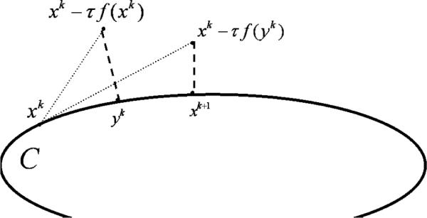
Korpelevich's iterative step.

Though convergence was proved in [1] under the assumptions of Lipschitz continuity and pseudo-monotonicity, there is still the need to calculate two projections onto C. If the set C is simple enough, so that projections onto it are easily executed, then this method is particularly useful; but, if C is a general closed and convex set, then a minimal distance problem has to be solved (twice) in order to obtain the next iterate. This might seriously affect the efficiency of the extragradient method. Therefore, we developed in [6] the subgradient extragradient algorithm in Euclidean space, in which we replace the (second) projection (3) onto C by a projection onto a specific constructible half-space, which is actually one of the subgradient half-spaces as will be explained later. In this paper, we study the subgradient extragradient method for solving the VI in Hilbert space. In addition, we present a modified version of the algorithm, which finds a solution of the VI that is also a fixed point of a given nonexpansive mapping. We establish weak convergence theorems for both algorithms.

Our paper is organized as follows. In Section 3, we sketch a proof of the weak convergence of the extragradient method. In Section 4, the subgradient extragradient algorithm is presented. It is analyzed in Section 5. In Section 6, we modify the subgradient extragradient algorithm and then analyze it in Section 7.

2 Preliminaries

Let H be a real Hilbert space with inner product 〈·, ·〉 and norm ∥ · ∥, and let D be a nonempty, closed and convex subset of H. We write x^k ⇀ x to indicate that the sequence ${\left\{x^k\right\}}_{k=0}^{\infty }$ converges weakly to x and x^k → x to indicate that the sequence ${\left\{x^k\right\}}_{k=0}^{\infty }$ converges strongly to x. For each point x ∈ H, there exists a unique nearest point in D, denoted by P_D(x). That is,

$$\parallel x-P_D\left(x\right)\parallel \le \parallel x-y\parallel ,\forall y\in D.$$ (4)

The mapping P_D : H → D is called the metric projection of H onto D. It is well known that P_D is a nonexpansive mapping of H onto D, i.e.,

$$\parallel P_D\left(x\right)-P_D\left(y\right)\parallel \le \parallel x-y\parallel ,\forall x,y\in H.$$ (5)

The metric projection P_D is characterized [7, Section 3] by the following two properties:

$$P_D\left(x\right)\in D$$ (6)

and

$$\langle x-P_D\left(x\right),P_D\left(x\right)-y\rangle \ge 0,\forall x\in H,y\in D,$$ (7)

and if D is a hyperplane, then (7) becomes an equality. It follows that

$${\parallel x-y\parallel }^2\ge {\parallel x-P_D\left(x\right)\parallel }^2+{\parallel y-P_D\left(x\right)\parallel }^2,\forall x\in H,y\in D.$$ (8)

We denote by N_D (v) the normal cone of D, at v ∈ D, i.e.,

$$N_D\left(v\right)≔\left\{d\in H\mid \langle d,y-v\rangle \le 0,\forall y\in D\right\}.$$ (9)

We also recall that in a real Hilbert space H,

$${\parallel \lambda x+(1-\lambda )y\parallel }^2=\lambda {\parallel x\parallel }^2+(1-\lambda ){\parallel y\parallel }^2-\lambda (1-\lambda ){\parallel x-y\parallel }^2,$$ (10)

for all x, y ∈ H and λ ∈ [0, 1].

Definition 2.1 Let B : H ⇉ 2^H be a point-to-set operator defined on a real Hilbert space H. B is called a maximal monotone operator iff B is monotone, i.e.,

$$\langle u-v,x-y\rangle \ge 0,\forall u\in B\left(x\right)and\forall v\in B\left(y\right),$$ (11)

and the graph G(B) of B,

$$G\left(B\right)≔\left\{(x,u)\in H\times H\mid u\in B\left(x\right)\right\},$$ (12)

is not properly contained in the graph of any other monotone operator.

It is clear ([8, Theorem 3]) that a monotone mapping B is maximal if and only if, for any (x, u) ∈ H × H, if 〈u − v, x − y〉 ≥ 0 for all (v, y) ∈ G(B), then it follows that u ∈ B(x).

The next property is known as the Opial condition [9]. Any Hilbert space has this property.

Condition 2.1 (Opial) For any sequence ${\left\{x^k\right\}}_{k=0}^{\infty }$ in H that converges weakly to x (x^k ⇀ x),

$$\underset{k\to \infty }{\text{lim inf}}\parallel x^k-x\parallel <\underset{k\to \infty }{\text{lim inf}}\parallel x^k-y\parallel ,\forall y\ne x.$$ (13)

The next lemma was proved in [10, Lemma 3.2].

Lemma 2.1 Let H be a real Hilbert space and let D be a nonempty, closed and convex subset of H. Let the sequence ${\left\{x^k\right\}}_{k=0}^{\infty }\subset H$ be Fejér-monotone with respect to D, i.e., for every u ∈ D,

$$\parallel x^{k+1}-u\parallel \le \parallel x^k-u\parallel ,\forall k\ge 0.$$ (14)

Then ${\left\{P_D\left(x^k\right)\right\}}_{k=0}^{\infty }$ converges strongly to some z ∈ D.

Notation 2.1 Any closed and convex set D ⊂ H can be represented as

$$D=\left\{x\in H\mid c\left(x\right)\le 0\right\},$$ (15)

where c : H → R is an appropriate convex function.

We denote the subdifferential set of c at a point x by

$$\partial c\left(x\right)≔\left\{\xi \in H\mid c\left(y\right)\ge c\left(x\right)+\langle \xi ,y-x\rangle ,\forall y\in H\right\}.$$ (16)

For z ∈ H, take any ξ ∈ ∂c(z) and define

$$T\left(z\right)≔\left\{w\in H\mid c\left(z\right)+\langle \xi ,w-z\rangle \le 0\right\}.$$ (17)

This is a half-space the bounding hyperplane of which separates the set D from the point z if z ∉ int D. Otherwise T(z) = H.

The next lemma is known (see, e.g., [11, Lemma 3.1]).

Lemma 2.2 Let H be a real Hilbert space, ${\left\{{\alpha }_k\right\}}_{k=0}^{\infty }$ a real sequence satisfying 0 < a ≤ α_k ≤ b < 1 for all k ≥ 0, and let ${\left\{{\upsilon }^k\right\}}_{k=0}^{\infty }$ and ${\left\{w^k\right\}}_{k=0}^{\infty }$ be two sequences in H such that for some σ ≥ 0,

$$\underset{k\to \infty }{\text{lim sup}}\parallel v^k\parallel \le \sigma ,$$ (18)

$$\underset{k\to \infty }{\text{lim sup}}\parallel w^k\parallel \le \sigma$$ (19)

and

$$\underset{k\to \infty }{\text{lim}}\parallel {\alpha }_k{v}^k+(1-{\alpha }_k)w^k\parallel =\sigma .$$ (20)

Then

$$\underset{k\to \infty }{\text{lim}}\parallel v^k-w^k\parallel =0.$$ (21)

The next fact is known as the Demiclosedness Principle [12].

Demiclosedness Principle. Let H be a real Hilbert space, D a closed and convex subset of H and let S : D → H be a nonexpansive mapping, i.e.,

$$\parallel S\left(x\right)-S\left(y\right)\parallel \le \parallel x-y\parallel ,\forall x,y\in D.$$ (22)

Then I − S (I is the identity operator on H) is demiclosed at y ∈ H, i.e., for any sequence ${\left\{x^k\right\}}_{k=0}^{\infty }$ in D such that $x^k\rightharpoonup \stackrel{‒}{x}\in D$ and (I − S)x^k → y, we have $(I-S)\stackrel{‒}{x}=y$.

3 The Extragradient Algorithm

In this section we sketch the proof of the weak convergence of Korpelevich's extragradient method, (2)−(3).

We assume the following conditions.

Condition 3.1 The solution set of (1), denoted by SOL(C, f), is nonempty.

Condition 3.2 The mapping f is monotone on C, i.e.,

$$\langle f\left(x\right)-f\left(y\right),x-y\rangle \ge 0,\forall x,y\in C.$$ (23)

Condition 3.3 The mapping f is Lipschitz continuous on C with constant L > 0, that is,

$$\parallel f\left(x\right)-f\left(y\right)\parallel \le L\parallel x-y\parallel ,\forall x,y\in C.$$ (24)

We will use the same outline in Section 5. The next lemma is a known result which is crucial for the proof of our convergence theorem.

Lemma 3.1 Let ${\left\{x^k\right\}}_{k=0}^{\infty }$ and ${\left\{y^k\right\}}_{k=0}^{\infty }$ be the two sequences generated by the extragradient method, (2)–(3), and let u ∈ SOL(C, f). Then, under Conditions 3.1–3.3, we have

$${\parallel x^{k+1}-u\parallel }^2\le {\parallel x^k-u\parallel }^2-(1-{\tau }^2{L}^2){\parallel y^k-x^k\parallel }^2,\forall k\ge 0.$$ (25)

Proof. see, e.g., [1, Theorem 1, eq. (14)], [2, Lemma 12.1.10, p. 1117]

Theorem 3.1 Assume that Conditions 3.1–3.3 hold and let τ < 1/L. Then any sequences ${\left\{x^k\right\}}_{k=0}^{\infty }$ and ${\left\{y^k\right\}}_{k=0}^{\infty }$ generated by the extragradient method weakly converge to the same solution u* ∈ SOL(C, f) and furthermore,

$$u\ast =\underset{k\to \infty }{\text{lim}}{P}_{SOL(C,f)}\left(x^k\right).$$ (26)

Proof. Fix u ∈ SOL(C, f) and define ρ := 1 − τ²L². Since τ < 1/L, ρ ∈ (0, 1). By (25), we have

$$\rho {\parallel y^k-x^k\parallel }^2\le {\parallel x^k-u\parallel }^2.$$ (27)

Using (25) with k ← (k − 1), we get

$$\rho {\parallel y^k-x^k\parallel }^2+\rho {\parallel y^{k-1}-x^{k-1}\parallel }^2\le {\parallel x^{k-1}-u\parallel }^2.$$ (28)

Continuing, we get for all integers K ≥ 0,

$$\rho \sum _{k=0}^K{\parallel y^k-x^k\parallel }^2\le {\parallel x^0-u\parallel }^2$$ (29)

and therefore

$$\rho \sum _{k=0}^{\infty }{\parallel y^k-x^k\parallel }^2\le {\parallel x^0-u\parallel }^2.$$ (30)

Hence

$$\underset{k\to \infty }{\text{lim}}\parallel y^k-x^k\parallel =0.$$ (31)

By Lemma 3.1, the sequence ${\left\{x^k\right\}}_{k=0}^{\infty }$ is bounded. Therefore it has at least one weak accumulation point. If $\stackrel{‒}{x}$ is a weak limit point of some subsequence ${\left\{x^{k_j}\right\}}_{j=0}^{\infty }$ of ${\left\{x^k\right\}}_{k=0}^{\infty }$, then

$$\mathrm{w}-\underset{j\to \infty }{\text{lim}}{x}^{k_j}=\stackrel{‒}{x}$$ (32)

and

$$\mathrm{w}-\underset{j\to \infty }{\text{lim}}{y}^{k_j}=\stackrel{‒}{x}.$$ (33)

Let

$$A\left(v\right)\{\begin{array}{cc}\hfill f\left(v\right)+N_C\left(v\right),\hfill & \hfill v\in C,\hfill \\ \hfill \varnothing ,\hfill & \hfill v\notin C,\hfill \end{array}\phantom{\}}$$ (34)

where N_C (v) is the normal cone of C at v ∈ C (see 9). It is known that A is a maximal monotone operator and A⁻¹ (0) = SOL(f, C). If (v, w) ∈ G(A), then

$$(w,v-\stackrel{‒}{x})\ge 0,$$ (35)

and therefore $\stackrel{‒}{x}\in A^{-1}\left(0\right)=\mathrm{SOL}(f,C)$. The Opial condition now implies that the entire sequence weakly converges to $\stackrel{‒}{x}$. Finally, if we take

$$u^k=P_{SOL(C,f)}\left(x^k\right),$$ (36)

then by (7) and Lemma 2.1, we see that ${\left\{u^k\right\}}_{k=0}^{\infty }$ converges strongly to some u* ∈ SOL(C, f). We also heve

$$\langle \stackrel{‒}{x}-u\ast ,u\ast -\stackrel{‒}{x}\rangle \ge 0,$$ (37)

and hence u* = $\stackrel{‒}{x}$, which completes the proof.

4 The Subgradient Extragradient Algorithm

Next we present the subgradient extragradient algorithm [6].

Algorithm 4.1 The subgradient extragradient algorithm

Step 0: Select a starting point x⁰ ∈ H and τ > 0, and set k = 0.

Step 1: Given the current iterate x^k, compute

$$y^k=P_C(x^k-\tau f\left(x^k\right))$$ (38)

construct the half-space T_k the bounding hyperplane of which supports C at y^k,

$$T_K≔\left\{w\in H\mid \langle (x^k-\tau f\left(x^k\right))-y^k,w-y^k\rangle \le 0\right\}$$ (39)

and calculate the next iterate

$$x^{k+1}=P_{T_k}(x^k-\tau f\left(y^k\right)).$$ (40)

Step 2: If x^k = y^k then stop. Otherwise, set k ← (k + 1) and return to Step 1.

Remark 4.1 Every convex set C can be represented as a sublevel set of a convex function c : H → R as in (15); so if c is, in addition, differentiable at y^k, then {(x^k − τf(x^k)) − y^k} = ∂c(y^k) = {∇c(y^k)}. Otherwise, (x^k − τf(x^k)) − y^k ∈ ∂c(y^k).

Figure 2 illustrates the iterative step of this algorithm.

Figure 2.

x^k+1 is a subgradient projection of the point x^k − τf(y^k) onto the hyperplane T_k.

We assume the following condition.

Condition 4.1 The function f is Lipschitz continuous on H with constant L > 0, that is,

$$\parallel f\left(x\right)-f\left(y\right)\parallel \le L\parallel x-y\parallel ,\forall x,y\in H.$$ (41)

5 Convergence of the Subgradient Extragradient Algorithm

In this section we give a complete proof of the weak convergence theorem for Algorithm 4.1, using similar techniques to those sketched in Section 3. First we show that the stopping criterion in Step 2 of Algorithm 4.1 is valid.

Lemma 5.1 If x^k = y^k in Algorithm 4.1, then x^k ∈ SOL(C, f).

Proof. If x^k = y^k, then x^k = P_C(x^k−τf(x^k)), so x^k ∈ C. By the variational characterization of the metric projection onto C, we have

$$\langle w-x^k,(x^k-\tau f\left(x^k\right))-x^k\rangle \le 0,\forall w\in C,$$ (42)

which implies that

$$\tau \langle f\left(x^k\right),w-x^k\rangle \ge 0,\forall w\in C.$$ (43)

Since τ > 0, inequality (43) implies that x^k ∈ SOL(C, f).

The next lemma is crucial for the proof of our convergence theorem.

Lemma 5.2 Let ${\left\{x^k\right\}}_{k=0}^{\infty }$ and ${\left\{y^k\right\}}_{k=0}^{\infty }$ be the two sequences generated by Algorithm 4.1 and let u ∈ SOL(C, f). Then, under Conditions 3.1, 3.2 and 4.1, we have

$${\parallel x^{k+1}-u\parallel }^2\le {\parallel x^k-u\parallel }^2-(1-{\tau }^2{L}^2){\parallel y^k-x^k\parallel }^2,\forall k\ge 0.$$ (44)

Proof. Since u ∈ SOL(C, f), y^k ∈ C and f is monotone, we have

$$\langle f\left(y^k\right)-f\left(u\right),y^k-u\rangle \ge 0,\forall k\ge 0.$$ (45)

This implies that

$$\langle f\left(y^k\right),y^k-u\rangle \ge 0,\forall k\ge 0.$$ (46)

So,

$$\langle f\left(y^k\right),x^{k+1}-u\rangle \ge \langle f\left(y^k\right),x^{k+1}-y^k\rangle .$$ (47)

By the variational characterization of the metric projection onto T_k, we have

$$\langle x^{k+1}-y^k,(x^k-\tau f\left(x^k\right))-y^k\rangle =0$$ (48)

for all k ≥ 0: Thus,

$$\begin{array}{cc}\hfill \langle x^{k+1}-y^k,(x^k-\tau f\left(x^k\right))-y^k\rangle & =\langle x^{k+1}-y^k,x^k-\tau f\left(x^k\right)-y^k\rangle \hfill \\ \hfill & +\tau \langle x^{k+1}-y^k,f\left(x^k\right)-f\left(y^k\right)\rangle \hfill \\ \hfill & =\tau \langle x^{k+1}-y^k,f\left(x^k\right)-f\left(y^k\right)\rangle .\hfill \end{array}$$ (49)

Denoting z^k = x^k = ^k − τf(y^k), we obtain

$$\begin{array}{cc}\hfill {\parallel x^{k+1}-u\parallel }^2& ={\parallel P_{T_k}\left(z^k\right)-u\parallel }^2\hfill \\ \hfill & =\langle P_{T_k}\left(z^k\right)-z^k+z^k-u,P_{T_k}\left(z^k\right)-z^k+z^k-u\rangle \hfill \\ \hfill & ={\parallel z^k-u\parallel }^2{\parallel z^k-P_{T_k}\left(z^k\right)\parallel }^2+2\langle P_{T_k}\left(z^k\right)-z^k,z^k-u\rangle .\hfill \end{array}$$ (50)

Since

$$\begin{array}{cc}\hfill 2& {\parallel z^k-P_{T_k}\left(z^k\right)\parallel }^2+2\langle P_{T_k}\left(z^k\right)-z^k,z^k-u\rangle \hfill \\ \hfill & =2\langle z^k-P_{T_k}\left(z^k\right),u-P_{T_k}\left(z^k\right)\rangle \le 0\hfill \end{array}$$ (51)

for all k ≥ 0, we get

$${\parallel z^k-P_{T_k}\left(z^k\right)\parallel }^2+2\langle P_{T_k}\left(z^k\right)-z^k,z^k-u\rangle \le -{\parallel z^k-P_{T_k}\left(z^k\right)\parallel }^2$$ (52)

for all k ≥ 0. Hence,

$$\begin{array}{cc}\hfill {\parallel x^{k+1}-u\parallel }^2& \le {\parallel z^k-u\parallel }^2-{\parallel z^k-P_{T_k}\left(z^k\right)\parallel }^2\hfill \\ \hfill & ={\parallel (x^k-\tau f\left(y^k\right))-u\parallel }^2-{\parallel (x^k-\tau f\left(y^k\right))-x^{k+1}\parallel }^2\hfill \\ \hfill & ={\parallel x^k-u\parallel }^2-{\parallel x^k-x^{k+1}\parallel }^2+2\tau \langle u-x^{k+1},f\left(y^k\right)\rangle \hfill \\ \hfill & \le {\parallel x^k-u\parallel }^2-{\parallel x^k-x^{k+1}\parallel }^2+2\tau \langle y^k-x^{k+1},f\left(y^k\right)\rangle ,\hfill \end{array}$$ (53)

where the last inequality follows from (47). So,

$$\begin{array}{cc}\hfill {\parallel x^{k+1}-u\parallel }^2& \le {\parallel x^k-u\parallel }^2-{\parallel x^k-x^{k+1}\parallel }^2+2\tau \langle y^k-x^{k+1},f\left(y^k\right)\rangle \hfill \\ \hfill & ={\parallel x^k-u\parallel }^2-\left(\langle x^k-y^k+y^k-x^{k+1},x^k-y^k+y^k-x^{k+1}\rangle \right)\hfill \\ \hfill & +2\tau \langle y^k-x^{k+1},f\left(y^k\right)\rangle \hfill \\ \hfill & ={\parallel x^k-u\parallel }^2-{\parallel x^k-y^k\parallel }^2-{\parallel y^k-x^{k+1}\parallel }^2\hfill \\ \hfill & +2\langle x^{k+1}-y^k,x^k-\tau f\left(y^k\right)-y^k\rangle ,\hfill \end{array}$$ (54)

and by (49),

$$\begin{array}{cc}\hfill {\parallel x^{k+1}-u\parallel }^2& \le {\parallel x^k-u\parallel }^2-{\parallel x^k-y^k\parallel }^2-{\parallel y^k-x^{k+1}\parallel }^2\hfill \\ \hfill & +2\tau \langle x^{k+1}-y^k,f\left(x^k\right)-f\left(y^k\right)\rangle .\hfill \end{array}$$ (55)

Using the Cauchy–Schwarz inequality and Condition 4.1, we obtain

$$2\tau \langle x^{k+1}-y^k,f\left(x^k\right)-f\left(y^k\right)\rangle \le 2\tau L\parallel x^{k+1}-y^k\parallel \parallel x^k-y^k\parallel .$$ (56)

In addition,

$$\begin{array}{cc}\hfill 0& \le {\left(\tau L\parallel x^k-y^k\parallel -\parallel y^k-x^{k+1}\parallel \right)}^2\hfill \\ \hfill & ={\tau }^2{L}^2{\parallel x^k-y^k\parallel }^2-2\tau L\parallel x^{k+1}-y^k\parallel \parallel x^k-y^k\parallel +{\parallel y^k-x^{k+1}\parallel }^2.\hfill \end{array}$$ (57)

So,

$$2\tau L\parallel x^{k+1}-y^k\parallel \parallel x^k-y^k\parallel \le {\tau }^2{L}^2{\parallel x^k-y^k\parallel }^2+{\parallel y^k-x^{k+1}\parallel }^2.$$ (58)

Combining the above inequalities and using Condition 4.1, we see that

$$\begin{array}{cc}\hfill {\parallel x^{k+1}-u\parallel }^2& \le {\parallel x^k-u\parallel }^2-{\parallel x^k-y^k\parallel }^2-{\parallel y^k-x^{k+1}\parallel }^2\hfill \\ \hfill & +2\tau L\parallel x^{k+1}-y^k\parallel \parallel x^k-y^k\parallel \hfill \\ \hfill & \le {\parallel x^k-u\parallel }^2-{\parallel x^k-y^k\parallel }^2-{\parallel y^k-x^{k+1}\parallel }^2\hfill \\ \hfill & +{\tau }^2{L}^2\parallel x^k-y^k\parallel +{\parallel y^k-x^{k+1}\parallel }^2\hfill \\ \hfill & ={\parallel x^k-u\parallel }^2-{\parallel x^k-y^k\parallel }^2+{\tau }^2{L}^2{\parallel x^k-y^k\parallel }^2.\hfill \end{array}$$ (59)

Finally, we get

$${\parallel x^{k+1}-u\parallel }^2\le {\parallel x^k-u\parallel }^2-(1-{\tau }^2{L}^2){\parallel y^k-x^k\parallel }^2,$$ (60)

which completes the proof.

Theorem 5.1 Assume that Conditions 3.1, 3.2 and 4.1 hold and let τ < 1/L. Then any sequences ${\left\{x^k\right\}}_{k=0}^{\infty }$ and ${\left\{y^k\right\}}_{k=0}^{\infty }$ generated by Algorithm 4.1 weakly converge to the same solution z* ∈ SOL(C, F) and furthermore,

$$u\ast =\underset{k\to \infty }{\text{lim}}{P}_{SOL(C,f)}\left(x^k\right).$$ (61)

Proof. Fix u ∈ SOL(C, f) and define ρ := 1 − τ²L². Since τ < 1/L, ρ ∈ (0, 1). By (60), we have

$$0\le {\parallel x^k-u\parallel }^2-\rho {\parallel y^k-x^k\parallel }^2,$$ (62)

or

$$\rho {\parallel y^k-x^k\parallel }^2\le {\parallel x^k-u\parallel }^2.$$ (63)

Using (60) with k ← (k − 1), we get

$${\parallel x^k-u\parallel }^2\le {\parallel x^{k-1}-u\parallel }^2-\rho {\parallel y^{k-1}-x^{k-1}\parallel }^2,$$ (64)

or

$$\rho {\parallel y^k-x^k\parallel }^2+\rho {\parallel y^{k-1}-x^{k-1}\parallel }^2\le {\parallel x^{k-1}-u\parallel }^2.$$ (65)

Continuing, we get for all integers K ≥ 0,

$$\rho \sum _{k=0}^K{\parallel y^k-x^k\parallel }^2\le {\parallel x^0-u\parallel }^2.$$ (66)

Since the sequence ${\left\{{\Sigma }_{k=0}^K{\parallel y^k-x^k\parallel }^2\right\}}_{K\ge 0}$ is monotonically increasing and bounded,

$$\rho \sum _{k=0}^{\infty }{\parallel y^k-x^k\parallel }^2\le {\parallel x^0-u\parallel }^2.$$ (67)

Hence

$$\underset{k\to \infty }{\text{lim}}\parallel y^k-x^k\parallel =0.$$ (68)

By Lemma 5.2, the sequence ${\left\{x^k\right\}}_{k=0}^{\infty }$ is bounded. Therefore, it has at least one weak accumulation point. If $\stackrel{‒}{x}$ is a weak limit point of some subsequence ${\left\{x^{k_j}\right\}}_{j=0}^{\infty }$ of ${\left\{x^k\right\}}_{k=0}^{\infty }$, then

$$\mathrm{w}-\underset{j\to \infty }{\text{lim}}{x}^{k_j}=\stackrel{‒}{x}$$ (69)

and

$$\mathrm{w}-\underset{j\to \infty }{\text{lim}}{y}^{k_j}=\stackrel{‒}{x}.$$ (70)

Define the operator A by (34). It is known that A is a maximal monotone operator and A⁻¹ (0) = SOL(f; C). If (v; w) ∈ G (A), since w ∈ A(v) = f(v) + N_C (v), we get w − f(v) ∈ N_C (v). Then

$$\langle w-f\left(v\right),v-y\rangle \ge 0,\forall y\in C.$$ (71)

On the other hand, by the definition of y^k and (7),

$$\langle x^k-\tau f\left(x^k\right)-y^k,y^k-v\rangle \ge 0,$$ (72)

or

$$\langle \left(\frac{y^k-x^k}{\tau }\right)+f\left(x^k\right),v-y^k\rangle \ge 0$$ (73)

for all k ≥ 0. Using (68) and applying (71) with ${\left\{y^{k_j}\right\}}_{j=0}^{\infty }$, we get

$$\langle w-f\left(v\right),v-y^{k_j}\rangle \ge 0.$$ (74)

Hence,

$$\begin{array}{cc}\hfill \langle w,v-y^{k_j}\rangle & \ge \langle f\left(v\right),v-y^{k_j}\rangle \ge \langle f\left(v\right),v-y^{k_j}\rangle \hfill \\ \hfill & -\langle \left(\frac{y^{k_j}-x^{k_j}}{\tau }\right)+f\left(x^{k_j}\right),v-y^{k_j}\rangle \hfill \\ \hfill & =\langle f\left(v\right)-f\left(y^{k_j}\right),v-y^{k_j}\rangle +\langle f\left(y^{k_j}\right)-f\left(x^{k_j}\right),v-y^{k_j}\rangle \hfill \\ \hfill & -\langle \left(\frac{y^{k_j}-x^{k_j}}{\tau }\right),v-y^{k_j}\rangle \hfill \\ \hfill & \ge \langle f\left(y^{k_j}\right)-f\left(x^{k_j}\right),v-y^{k_j}\rangle -\langle \left(\frac{y^{k_j}-x^{k_j}}{\tau }\right),v-y^{k_j}\rangle \hfill \end{array}$$ (75)

and

$$\langle w,v-y^{k_j}\rangle \ge \langle f\left(y^{k_j}\right)-f\left(x^{k_j}\right),v-y^{k_j}\rangle -\langle \left(\frac{y^{k_j}-x^{k_j}}{\tau }\right),v-y^{k_j}\rangle .$$ (76)

Taking the limit as j → ∞, we obtain

$$\langle w,v-\stackrel{‒}{x})\ge 0,$$ (77)

and since A is a maximal monotone operator, it follows that $\stackrel{‒}{x}\in A^{-1}\left(0\right)=SOL(f,C)$. In order to show that the entire sequence weakly converges to $\stackrel{‒}{x}$, assume that there is another subsequence ${\left\{x^{{\stackrel{‒}{k}}_j}\right\}}_{j=0}^{\infty }$ of ${\left\{x^k\right\}}_{k=0}^{\infty }$ that weakly converges to some ${\stackrel{‒}{x}}^{\prime }\ne \stackrel{‒}{x}$ and ${\stackrel{‒}{x}}^{\prime }\in \text{SOL}(f,C)$ ∈ SOL(f, C). Note that from Lemma 5.2 it follows that the sequence ${\left\{\parallel x^k-\stackrel{‒}{x}\parallel \right\}}_{k=0}^{\infty }$ is decreasing for each u ∈ SOL(C, f). By the Opial condition we have

$$\begin{array}{cc}\hfill \underset{k\to \infty }{\text{lim}}\parallel x^k-\stackrel{‒}{x}\parallel & =\underset{j\to \infty }{\text{lim inf}}\parallel x^{k_j}-\stackrel{‒}{x}\parallel <\underset{j\to \infty }{\text{lim inf}}\parallel x^{k_j}-{\stackrel{‒}{x}}^{\prime }\parallel \hfill \\ \hfill & =\underset{k\to \infty }{\text{lim}}\parallel x^k-{\stackrel{‒}{x}}^{\prime }\parallel =\underset{j\to \infty }{\text{lim inf}}\parallel x^{{\stackrel{‒}{k}}_j}-{\stackrel{‒}{x}}^{\prime }\parallel <\underset{j\to \infty }{\text{lim inf}}\parallel x^{{\stackrel{‒}{k}}_j}-{\stackrel{‒}{x}}^{\prime }\parallel \hfill \\ \hfill & =\underset{k\to \infty }{\text{lim}}\parallel x^k-\stackrel{‒}{x}\parallel ,\hfill \end{array}$$ (78)

and this is a contradiction, thus ${\stackrel{‒}{x}}^{\prime }=\stackrel{‒}{x}$. This implies that the sequences ${\left\{x^k\right\}}_{k=0}^{\infty }$ and ${\left\{y^k\right\}}_{k=0}^{\infty }$ converge weakly to the same point $\stackrel{‒}{x}\in \text{SOL}(C,f)$. Finally, put

$$u^k=P_{SOL(C,f)}\left(x^k\right),$$ (79)

so by (7) and since $\stackrel{‒}{x}\in \text{SOL}(C,f)$,

$$\langle \stackrel{‒}{x}-u^k,u^k-x^k\rangle \ge 0.$$ (80)

By Lemma 2.1, ${\left\{u^k\right\}}_{k=0}^{\infty }$ converges strongly to some u* ∈ SOL(C, f). Therefore

$$\langle \stackrel{‒}{x}-u\ast ,u\ast -\stackrel{‒}{x}\rangle \ge 0$$ (81)

and hence $u\ast =\stackrel{‒}{x}$.

6 The Modified Subgradient Extragradient Algorithm

Next we present the modified subgradient extragradient algorithm which finds a solution of the VI which is also a fixed point of a given nonexpansive mapping. Let S : H → H be a nonexpansive mapping and denote by Fix(S) its fixed point set, i.e.,

$$\text{Fix}\left(S\right)=\left\{x\in H\mid S\left(x\right)=x\right\}.$$ (82)

Let ${\left\{{\alpha }_k\right\}}_{k=0}^{\infty }\subset [c,d]$ for some c, d ∈ (0, 1).

Algorithm 6.1 The modified subgradient extragradient algorithm

Step 0: Select a starting point x⁰ ∈ H and τ > 0, and set k = 0.

Step 1: Given the current iterate x^k, compute

$$y^k-P_C(x^k-\tau f\left(x^k\right)),$$ (83)

construct the half-space T_k as in (39) and calculate the next iterate

$$x^{k+1}={\alpha }_k{x}^k+(1-{\alpha }_k)S{P}_{T_k}(x^k-\tau f\left(y^k\right)).$$ (84)

Step 2: Set k ← (k + 1) and return to Step 1.

Figure 3 illustrates the iterative step of this algorithm. We assume the following condition.

Figure 3.

The iterative step of Algorithm 6.1.

Condition 6.1 Fix(S) ∩ SOL(C, f) ≠ ∅.

7 Convergence of the Modified Subgradient Extragradient Algorithm

In this section we establish a weak convergence theorem for Algorithm 6.1. The outline of its proof is similar to that of [11, Theorem 3.1].

Theorem 7.1 Assume that Conditions 3.2, 4.1 and 6.1 hold and τ < 1/L. Then any sequences ${\left\{x^k\right\}}_{k=0}^{\infty }$ and ${\left\{y^k\right\}}_{k=0}^{\infty }$ generated by Algorithm 6.1 weakly converge to the same point u* ∈ Fix(S) ∩ SOL(C, f) and furthermore,

$$u\ast =\underset{k\to \infty }{\text{lim}}{P}_{\text{Fix}\left(S\right)\cap SOL(C,f)}\left(x^k\right).$$ (85)

Proof. Denote t^k := P_Tk (x^k − τf(y^k)) for all k ≥ 0. Let u ∈ Fix(S) ∩ SOL(C, f). Applying (8) with D = T_k, x = x^k − τf(y^k) and y = u, we obtain

$$\begin{array}{cc}\hfill {\parallel t^k-u\parallel }^2& \le {\parallel x^k-\tau f\left(y^k\right)-u\parallel }^2-{\parallel x^k-\tau f\left(y^k\right)-t^k\parallel }^2\hfill \\ \hfill & ={\parallel x^k-u\parallel }^2-{\parallel x^k-t^k\parallel }^2+2\tau \langle f\left(y^k\right),u-t^k\rangle \hfill \\ \hfill & ={\parallel x^k-u\parallel }^2-{\parallel x^k-t^k\parallel }^2\hfill \\ \hfill & +2\tau \left(\langle f\left(y^k\right)-f\left(u\right),u-y^k\rangle +\langle f\left(u\right),u-y^k\rangle +\langle f\left(y^k\right),y^k-t^k\rangle \right).\hfill \end{array}$$ (86)

By Condition 3.2,

$$\langle f\left(y^k\right)-f\left(u\right),u-y^k\rangle \le 0,$$ (87)

and since u ∈ SOL(C, f)

$$\langle f\left(u\right),u-y^k\rangle \le 0.$$ (88)

So,

$$\begin{array}{cc}\hfill {\parallel t^k-u\parallel }^2& \le {\parallel x^k-u\parallel }^2-{\parallel x^k-t^k\parallel }^2+2\tau \langle f\left(y^k\right),y^k-t^k\rangle \hfill \\ \hfill & ={\parallel x^k-u\parallel }^2-{\parallel x^k-y^k\parallel }^2-2\langle x^k-y^k,y^k-t^k\rangle \hfill \\ \hfill & -{\parallel y^k-t^k\parallel }^2+2\tau \langle f\left(y^k\right),y^k-t^k\rangle \hfill \\ \hfill & ={\parallel x^k-u\parallel }^2-{\parallel x^k-y^k\parallel }^2-{\parallel y^k-t^k\parallel }^2\hfill \\ \hfill & +2\langle x^k-\tau f\left(y^k\right)-y^k,t^k-y^k\rangle .\hfill \end{array}$$ (89)

By (7) applied to T_k,

$$\langle (x^k-\tau f\left(x^k\right))-y^k,t^k-y^k\rangle =0,$$ (90)

so

$$\begin{array}{cc}\hfill & \langle x^k-\tau f\left(y^k\right)-y^k,t^k-y^k\rangle \hfill \\ \hfill & =\langle x^k-\tau f\left(x^k\right)-y^k,t^k-y^k\rangle +\langle \tau f\left(x^k\right)-\tau f\left(y^k\right),t^k-y^k\rangle \hfill \\ \hfill & =\langle \tau f\left(x^k\right)-\tau f\left(y^k\right),t^k-y^k\rangle \le \tau \parallel f\left(x^k\right)-f\left(y^k\right)\parallel \parallel t^k-y^k\parallel \hfill \\ \hfill & \le \tau L\parallel x^k-y^k\parallel \parallel t^k-y^k\parallel ,\hfill \end{array}$$ (91)

where the last two inequalities follow from the Cauchy–Schwarz inequality and Condition 4.1. Therefore

$${\parallel t^k-u\parallel }^2\le {\parallel x^k-u\parallel }^2-{\parallel x^k-y^k\parallel }^2-{\parallel y^k-t^k\parallel }^2+2\tau L\parallel x^k-y^k\parallel \parallel t^k-y^k\parallel .$$ (92)

Observe that

$$\begin{array}{cc}\hfill 0& \le {\left(\parallel t^k-y^k\parallel -\tau L\parallel t^k-y^k\parallel \right)}^2\hfill \\ \hfill & ={\parallel t^k-y^k\parallel }^2-2\tau L\parallel x^k-y^k\parallel \parallel t^k-y^k\parallel +{\tau }^2{L}^2{\parallel x^k-y^k\parallel }^2,\hfill \end{array}$$ (93)

so,

$$2\tau L\parallel x^k-y^k\parallel \parallel t^k-y^k\parallel \le {\parallel t^k-y^k\parallel }^2+{\tau }^2{L}^2{\parallel x^k-y^k\parallel }^2.$$ (94)

Thus

$$\begin{array}{cc}\hfill {\parallel t^k-u\parallel }^2& \le {\parallel x^k-u\parallel }^2-{\parallel x^k-y^k\parallel }^2-{\parallel y^k-t^k\parallel }^2\hfill \\ \hfill & +{\parallel t^k-y^k\parallel }^2+{\tau }^2{L}^2{\parallel x^k-y^k\parallel }^2\hfill \\ \hfill & ={\parallel x^k-u\parallel }^2-{\parallel x^k-y^k\parallel }^2+{\tau }^2{L}^2{\parallel x^k-y^k\parallel }^2\hfill \\ \hfill & ={\parallel x^k-u\parallel }^2+({\tau }^2{L}^2-1){\parallel x^k-y^k\parallel }^2\hfill \\ \hfill & \le {\parallel x^k-u\parallel }^2,\hfill \end{array}$$ (95)

where the last inequality follows from the fact that τ < 1/L. Using (10), we get

$$\begin{array}{cc}\hfill {\parallel x^{k+1}-u\parallel }^2& ={\parallel {\alpha }_k{x}^k+(1-{\alpha }_k)S\left(t^k\right)-u\parallel }^2\hfill \\ \hfill & ={\parallel {\alpha }_k(x^k-u)+(1-{\alpha }_k)(S\left(t^k\right)-u)\parallel }^2\hfill \\ \hfill & ={\alpha }_k{\parallel x^k-u\parallel }^2+(1-{\alpha }_k){\parallel S\left(t^k\right)-u\parallel }^2\hfill \\ \hfill & -{\alpha }_k(1-{\alpha }_k){\parallel (x^k-u)-(S\left(t^k\right)-u)\parallel }^2\hfill \\ \hfill & \le {\alpha }_k{\parallel x^k-u\parallel }^2+(1-{\alpha }_k){\parallel S\left(t^k\right)-u\parallel }^2\hfill \\ \hfill & ={\alpha }_k{\parallel x^k-u\parallel }^2+(1-{\alpha }_k){\parallel S\left(t^k\right)-S\left(u\right)\parallel }^2\hfill \\ \hfill & \le {\alpha }_k{\parallel x^k-u\parallel }^2+(1-{\alpha }_k){\parallel (t^k-u)\parallel }^2\hfill \\ \hfill & \le {\alpha }_k{\parallel x^k-u\parallel }^2+(1-{\alpha }_k)\left({\parallel x^k-u\parallel }^2+({\tau }^2{L}^2-1){\parallel x^k-y^k\parallel }^2\right)\hfill \\ \hfill & ={\parallel x^k-u\parallel }^2+(1-{\alpha }_k)({\tau }^2{L}^2-1){\parallel x^k-y^k\parallel }^2\le {\parallel x^k-u\parallel }^2,\hfill \end{array}$$ (96)

so

$${\parallel x^{k+1}-u\parallel }^2\le {\parallel x^k-u\parallel }^2.$$ (97)

Therefore there exists

$$\underset{k\to \infty }{\text{lim}}\parallel x^k-u\parallel =\sigma ,$$ (98)

and ${\left\{x^k\right\}}_{k=0}^{\infty }$ and ${\left\{t^k\right\}}_{k=0}^{\infty }$ are bounded. From the last relations it follows that

$$(1-{\alpha }_k)(1-{\tau }^2{L}^2){\parallel x^k-y^k\parallel }^2\le {\parallel x^k-u\parallel }^2-{\parallel x^{k+1}-u\parallel }^2,$$ (99)

or

$${\parallel x^k-y^k\parallel }^2\le \frac{{\parallel x^k-u\parallel }^2-{\parallel x^{k+1}-u\parallel }^2}{(1-{\alpha }_k)(1-{\tau }^2{L}^2)}.$$ (100)

Hence,

$$\underset{k\to \infty }{\text{lim}}\parallel x^k-y^k\parallel =0.$$ (101)

In addition, by the definition of y^k and T_k,

$$\begin{array}{cc}\hfill {\parallel y^k-t^2\parallel }^2& ={\parallel P_C(x^k-\tau f\left(x^k\right))-P_{T_k}(x^k-\tau f\left(y^k\right))\parallel }^2\hfill \\ \hfill & ={\parallel P_{T_k}(x^k-\tau f\left(x^k\right))-P_{T_k}(x^k-\tau f\left(y^k\right))\parallel }^2\hfill \\ \hfill & \le {\parallel (x^k-\tau f\left(x^k\right))-(x^k-\tau f\left(y^k\right))\parallel }^2\hfill \\ \hfill & ={\parallel \tau f\left(y^k\right)-\tau f\left(x^k\right)\parallel }^2\hfill \\ \hfill & \le {\tau }^2{L}^{}{\parallel y^k-x^k\parallel }^2,\hfill \end{array}$$ (102)

where the last inequality follows from Condition 4.1. So,

$${\parallel y^k-t^k\parallel }^2\le {\tau }^2{L}^2{\parallel y^k-x^k\parallel }^2,$$ (103)

and by (101) we get

$$\underset{k\to \infty }{\text{lim}}\parallel y^k-t^k\parallel =0.$$ (104)

By the triangle inequality,

$$\parallel x^k-t^k\parallel \le \parallel x^k-y^k\parallel +\parallel y^k-t^k\parallel ,$$ (105)

so by (101) and (104), we have

$$\underset{k\to \infty }{\text{lim}}\parallel x^k-t^k\parallel =0.$$ (106)

Since ${\left\{x^k\right\}}_{k=0}^{\infty }$ is bounded, it has a subsequence ${\left\{x^{k_j}\right\}}_{j=0}^{\infty }$ which weakly converges to some $\stackrel{‒}{x}\in H$. We now show that $\stackrel{‒}{x}\in \text{Fix}\left(S\right)\cap \text{SOL}(C,f)$. Define the operator A as in (34). By using arguments similar to those used in the proof of Theorem 5.1, we get that $\stackrel{‒}{x}\in A^{-1}\left(0\right)=\text{SOL}(C,f)$. It is now left to show that $\stackrel{‒}{x}\in \text{Fix}\left(S\right)$. To this end, let $u\in \text{Fix}\left(S\right)\cap \text{SOL}(C,f)$ as before. Since S is nonexpansive, we get from (95) that

$$\parallel S\left(t^k\right)-u\parallel =\parallel S\left(t^k\right)-S\left(u\right)\parallel \le \parallel t^k-u\parallel \le \parallel x^k-u\parallel .$$ (107)

By (98),

$$\underset{k\to \infty }{\text{lim sup}}S\parallel \left(t^k\right)-u\parallel \le \sigma .$$ (108)

Furthermore,

$$\begin{array}{cc}\hfill & \underset{k\to \infty }{\text{lim}}\parallel {\alpha }_k{x}^k+(1-{\alpha }_k)S\left(t^k\right)-u\parallel \hfill \\ \hfill & =\underset{k\to \infty }{\text{lim}}\parallel {\alpha }_k(x^k-u)+(1-{\alpha }_k)(S\left(t^k\right)-u)\parallel \hfill \\ \hfill & =\underset{k\to \infty }{\text{lim}}\parallel x^{k+1}-u\parallel =\sigma .\hfill \end{array}$$ (109)

So applying Lemma 2.2, we obtain

$$\underset{k\to \infty }{\text{lim}}\parallel S\left(t^k\right)-x^k\parallel =0.$$ (110)

Since

$$\begin{array}{cc}\hfill \parallel S\left(x^k\right)-x^k\parallel & =\parallel S\left(x^k\right)-S\left(t^k\right)+S\left(t^k\right)-x^k\parallel \hfill \\ \hfill & \le \parallel S\left(x^k\right)-S\left(t^k\right)\parallel +\parallel S\left(t^k\right)-x^k\parallel \hfill \\ \hfill & \le \parallel x^k-t^k\parallel +\parallel S\left(t^k\right)-x^k\parallel ,\hfill \end{array}$$ (111)

It follows from (106) and (110) that

$$\underset{k\to \infty }{\text{lim}}\parallel S\left(x^k\right)-x^k\parallel =0.$$ (112)

Since S is nonexpansive on H, $x^{k_j}\rightharpoonup \stackrel{‒}{x}$ and

$$\underset{j\to \infty }{\text{lim}}\parallel (I-S)\left(x^{k_j}\right)\parallel =\underset{k\to \infty }{\text{lim}}\parallel x^{k_j}-S\left(x^{k_j}\right)\parallel =0,$$ (113)

we obtain by the Demiclosedness Principle that $(I-S)\left(\stackrel{‒}{x}\right)=0$, which means that $\stackrel{‒}{x}\in \text{Fix}\left(S\right)$. Now, again by using similar arguments to those used in the proof of Theorem 5.1, we get that the entire sequence weakly converges to $\stackrel{‒}{x}$. Therefore the sequences ${\left\{x^k\right\}}_{k=0}^{\infty }$ and ${\left\{y^k\right\}}_{k=0}^{\infty }$ weakly converge to $\stackrel{‒}{x}\in \text{Fix}\left(S\right)\cap \text{SOL}(C,f)$. Finally, put

$$u^k=P_{\text{Fix}\left(S\right)\cap SOL(C,f)}\left(x^k\right).$$ (114)

Since $\stackrel{‒}{x}\in \text{Fix}\left(S\right)\cap \text{SOL}(C,f)$, it follows from (7) that

$$\langle \stackrel{‒}{x}-u^k,u^k-x^k\rangle \ge 0.$$ (115)

By Lemma 2.1, ${\left\{u^k\right\}}_{k=0}^{\infty }$ converges strongly to some u* ∈ Fix(S) ∩ SOL(C, f). Therefore

$$\langle \stackrel{‒}{x}-u\ast ,u\ast -\stackrel{‒}{x}\rangle \ge 0.$$ (116)

and hence $\stackrel{‒}{x}u\ast$.

Remark 7.1 In Algorithm 6.1 we assumed that S was a nonexpansive mapping on H. If it is defined only on C we can replace it by $\tilde{S}=S{P}_C$, which is a nonexpansive mapping on C. In this case the iterative step is as follows:

$$y^k=P_C(x^k-\tau f\left(x^k\right)),$$

construct the half-space T_k (39) and calculate the next iterate

$$x^{k+1}={\alpha }_k{x}^k+(1-{\alpha }_k)\tilde{S}{P}_{T_k}(x^k-\tau f\left(y^k\right).$$ (117)

8 Conclusions

In this paper we proposed two subgradient extragradient algorithms for solving variational inequalities in Hilbert space and established weak convergence theorems for both of them. The second algorithm finds a solution of a variational inequality which is also a fixed point of a given nonexpansive mapping.

References

- [1].Korpelevich GM. The extragradient method for finding saddle points and other problems. Ekonomika i Matematicheskie Metody. 1976;12:747–756. [Google Scholar]
- [2].Facchinei F, Pang JS. Finite-Dimensional Variational Inequalities and Complementarity Problems. Volume I and Volume II. Springer-Verlag; New York: 2003. [Google Scholar]
- [3].Iusem AN, Svaiter BF. A variant of Korpelevich's method for variational inequalities with a new search strategy. Optimization. 1997;42:309–321. [Google Scholar]
- [4].Khobotov EN. Modification of the extra-gradient method for solving variational inequalities and certain optimization problems. USSR Comput. Math. Math. Phys. 1989;27:120–127. [Google Scholar]
- [5].Solodov MV, Svaiter BF. A new projection method for variational inequality problems. SIAM J. Control Optim. 1999;37:765–776. [Google Scholar]
- [6].Censor Y, Gibali A, Reich S. Two extensions of Korpelevich's extra-gradient method for solving the variational inequality problem in Euclidean space. Technical Report. 2010 [Google Scholar]
- [7].Goebel K, Reich S. Uniform Convexity, Hyperbolic Geometry, and Non-expansive Mappings. Marcel Dekker; New York and Basel: 1984. [Google Scholar]
- [8].Rockafellar RT. On the maximality of sums of nonlinear monotone operators. Trans. Amer. Math. Soc. 1970;149:75–88. [Google Scholar]
- [9].Opial Z. Weak convergence of the sequence of successive approximations for nonexpansive mappings. Bull. Amer. Math. Soc. 1967;73:591–597. [Google Scholar]
- [10].Takahashi W, Toyoda M. Weak convergence theorems for nonexpansive mappings and monotone mappings. J. Optim. Theory Appl. 2003;118:417–428. [Google Scholar]
- [11].Nadezhkina N, Takahashi W. Weak convergence theorem by an extra-gradient method for nonexpansive mappings and monotone mappings. J. Optim. Theory Appl. 2006;128:191–201. [Google Scholar]
- [12].Browder FE. Fixed point theorems for noncompact mappings in Hilbert space. Proc. Natl. Acad. Sci. USA. 1965;53:1272–1276. doi: 10.1073/pnas.53.6.1272. [DOI] [PMC free article] [PubMed] [Google Scholar]