

Abstract
Visualization and analysis of the micro-architecture of brain parenchyma by means of magnetic resonance imaging is nowadays believed to be one of the most powerful tools used for the assessment of various cerebral conditions as well as for understanding the intracerebral connectivity. Unfortunately, the conventional diffusion tensor imaging (DTI) used for estimating the local orientations of neural fibers, is incapable of performing reliably in the situations when a voxel of interest accommodates multiple fiber tracts. In this case, a much more accurate analysis is possible using the high angular resolution diffusion imaging (HARDI) that represents local diffusion by its apparent coefficients measured as a discrete function of spatial orientations. In this note, a novel approach to enhancing and modeling the HARDI signals using multiresolution bases of spherical ridgelets is presented. In addition to its desirable properties of being adaptive, sparsifying, and efficiently computable, the proposed modeling leads to analytical computation of the orientation distribution functions associated with the measured diffusion, thereby providing a fast and robust analytical solution for q-ball imaging.
Index Terms: Q-ball imaging, orientation distribution function, spherical harmonics, ridgelets, multiresolution analysis
I. Introduction
The need for the development of more reliable and accurate diagnostic tools for predicting and monitoring cerebral and neurological disorders necessitates the invention of novel methods for imaging the structure of brain tissue along with the physiological parameters of its parenchyma. In this regard, diffusion-weighted magnetic resonance imaging (DW-MRI) offers the possibility of acquiring a multitude of exquisite details on the microstructure of cerebral tissue via measuring the diffusion of water molecules across the neural fiber tracts [1], [2]. The most advanced application of DW-MRI is certainly that of fiber tracking, which, in combination with functional MRI, seems to be opening a window on the important issue of intracerebral connectivity [3], [4].
The most conventional type of DW-MRI – known as diffusion tensor imaging (DTI) – is based on the assumption that, at each voxel of DW-MRI data, the diffusion of water molecules can be represented by a unimodal Gaussian distribution model [5], [6, Ch.5]. In spite of the fact that DTI provides a stable and computationally efficient way to estimate the orientation of local diffusion flows, its accuracy is known to deteriorate dramatically at the sites where the neural fibers (or bundles thereof) cross, touch upon each other, or diverge [7]-[12]. In such a case, for instance, two highly anisotropic diffusion flows crossing each other at an approximately right angle will be perceived by DTI as being isotropic.
The fiber crossing problem in DTI has prompted efforts to develop DW-MRI methodologies which are capable of discriminating between multiple diffusion flows (or, equivalently, neural fiber tracts) within a given voxel. One of such techniques is high angular resolution diffusion imaging (HARDI), which measures the diffusion directly by sampling the diffusion signal over a spherical shell in diffusion wavevector space [9], [10], [13], [14]. Despite its numerous advantages, however, until recently the extensive use of HARDI has been hampered by the absence of analytical tools necessary to relate HARDI signals to their underlying orientation distribution functions (ODF). To resolve the above problem, Tuch [15] has introduced the q-ball imaging method, in which ODFs are estimated by applying the Funk-Radon transform to numerically interpolated HARDI data. However, the susceptibility of this approach to both interpolation and measurement errors necessitated further research in this direction.
In a typical implementation, the process of q-ball imaging consists of two principal steps. First, at each voxel of HARDI data, samples of the corresponding diffusion signal are fitted using a continuous model of the form
| (1) |
where S2 denotes the unit sphere, u ∈ S2, and {ψk}k∈I is a set of functions of a predefined nature (see below). Subsequently, the signal S(u) is subjected to the Funk-Radon transform [16], resulting in an approximation of the corresponding ODF – the function whose modes indicate the directions of local diffusion flows. While applying the Funk-Radon transform suggests a standard modus operandi, the fitting procedure of the first step above admits a variety of possible solutions, depending on how one defines the set {ψk}k∈I [17]. In particular, the latter can be defined to be a set of parametric functions, such as probability density functions [18], [19], high-order tensors [20], or directional functions [21]. The parametric models are advantageous, for they usually result in a minimal number of terms in (1) (normally two or three), and since their parameters can often be used to directly deduce the directions of local diffusion flows (which is, after all, the most valuable output of q-ball imaging). On the other hand, fitting the parametric models requires minimizing non-convex functionals, which is noise-sensitive, computationally intensive, and prone to the problem of local minima. The need to predetermine the optimal number of fitting terms in (1) is known to be another disadvantage of using the models of this kind.
Another way to define the set {ψk}k∈I is by using non-parametric functions, which form a dense set in the space of diffusion signals. In particular, the applicability of spherical Fourier analysis to q-ball imaging was demonstrated in [10]-[12]. In these works, HARDI signals are approximated (in the least-square sense) by truncated series of spherical harmonics (SH), in which case the corresponding ODFs can be conveniently recovered by means of the Funk-Hecke formula, as detailed in [11], [22]. Although the SH-parameterization is stable and computationally efficient, it typically involves a relatively large number of SHs1, which undermines the effectiveness of using this method in applications requiring a substantial reduction in the data dimensionality (with machine learning and data mining being the standard examples of applications of the above type).
The above considerations indicate that there is still a need for bona fide methods of modeling the HARDI signals based on (1) for the purpose of q-ball imaging. One should realize, however, that merely fitting a model of type (1) to discrete HARDI data cannot extend the resolution of q-ball imaging beyond its intrinsic limit (as defined by the diffusivity of brain tissue and the parameters of diffusion-encoding gradients). On the other hand, the output of q-ball imaging can be used by a deconvolution algorithm [17], [23]-[26], which does have the ability to improve the resolution. It is, therefore, important to define the set {ψk}k∈I so that it will be capable of encoding the maximum of directional information contained in the data. Moreover, the design of {ψk}k∈I should be subjected to the additional constraint requiring (1) to involve as few terms as possible. In addition to its other advantages, such “minimality” can be taken advantage of to facilitate the performance of, e.g., classification [27] and segmentation [28] algorithms. Finally, from the numerical point of view, reconstruction of the ODFs should be stable, unique, and computationally efficient, which, in combinations with the other requirements mentioned above, justifies the definition of {ψk}k∈I as a (non-parametric) basis of spherical functions, whose shape is strongly correlated with the shape of HARDI signals. Introducing such a basis is the main objective of this paper.
The construction of the proposed basis follows the fundamental principles of multiresolution analysis on the unit sphere [29]-[32]. In particular, in this paper we develop the concept of spherical ridgelets following the conceptual lines defined in [33]. Apart from providing a numerical recipe for construction of the ridgelet basis, it is also shown how the latter can be used for efficiently approximating the HARDI signals by means of the orthogonal matching pursuit algorithm [34]. Finally, we demonstrate how the ridgelet approximations can be used for recovering the ODFs by means of analytical computations, which result in a compact and accurate representation of the directionality of neural fiber tracts.
It should be noted that the proposed ridgelet analysis is different from the one recently presented in [35], where the authors, in fact, use “flat” ridgelets applied to localized regions of the unit sphere. Moreover, our construction also differs from that in [36], where a ridgelet-like transformation is derived using some properties of the Riesz potentials. Thus, to the best of our knowledge, the proposed construction of spherical ridgelets as well as its use in medical imaging for analytically approximating the ODFs is reported in this paper for the first time (with the exception of a brief introduction of the main idea in [37]).
The organization of this paper is as follows. Section II provides some necessary preliminaries on q-ball imaging as well as a number of relevant results from the theory of spherical harmonics. Section III presents a motivating example which justifies the construction of spherical ridgelets detailed in Section IV. A summary of the algorithm used for approximating the HARDI signals by spherical ridgelets is given in Section V, while Section VI demonstrates some results obtained in both in silico and in vivo experiments. Section VII finalizes the paper with a discussion and conclusions.
II. Background
A. Diffusion function and ODF
In diffusion MRI, the diffusion function P(r) : ℝ3 → ℝ+, defines the ensemble-averaged probability for a spin to undergo a relative displacement r = x − x0 (w. r. t. some reference point x0 ∈ ℝ3) in the experimental diffusion time τ. The orientation structure of the diffusion function can be described using the diffusion orientation distribution function (ODF) ψ(u) which is defined as the radial projection of P(r), viz. [15]
| (2) |
with u being a point (direction) on the unit sphere, i.e. u ∈ Ω ≡ S2, and Z standing for a normalization constant.
The basis of q-ball imaging is formed by the fact that ψ(u) can be closely approximated by the Funk-Radon transform R of the raw HARDI signal evaluated on the unit sphere Ω in the q-space, viz. [15]
| (3) |
where S is the HARDI signal, δ(·) is the delta function, the dot denotes the standard (Euclidean) inner product in ℝ3, and dη denotes the standard rotation invariant measure on Ω. Let σ (u) be a great circle with pole u, defined as the intersection of Ω with a 3-D plane through the origin of ℝ3, orthogonal to u. Then, the Funk-Radon transform of S is, in fact, its integral over all possible σ (u).
Finally, it should be noted that, under some general assumptions (see, e.g., [17, Sect. 3.1] for more details), the diffusion signal S(u) which originates from a voxel containing M fibers can be represented by the multi-tensor model as given by2
| (4) |
where Dk is a 3 × 3 (symmetric, positive definite) diffusion tensor associated with the k-th fiber, b > 0 is a constant defined by the diffusion time as well as by the amplitude and duration of diffusion-encoding gradients [6, Eq. 3.18], e(u) accounts for both measurement and model noises, and {pk} are proportionality constants obeying . Thus, the model of (4) represents the diffusion signal S(u) as a noise-contamined superposition of M unimodal Gaussian signals Sk(u) = exp{−b(uTDku)}, which pertain to different diffusion flows through the voxel of interest.
B. Spherical Harmonics and Related Theorems
In the sections that follow we will be mainly concerned with the space L2(Ω) of square-integrable functions on the unit sphere Ω. This space is a Hilbert space (with the standard definition of the inner product) that possesses an orthonormal basis of spherical harmonics {Yn,l}, with n ∈ ℕ and l = 1,…, 2n + 1 being the degree and the phase index of Yn,l, respectively. It is worthwhile noting that the spherical harmonics of degree n are defined as the eigenfunctions of the Beltrami operator ΔΩ on Ω with respect to the eigenvalue −n(n+1). Let us collect all spherical harmonics of the same degree n, and define . Also, let . Then, it can be rigorously proven that the closure of Harm0,…,m converges to L2(Ω), as m → ∞ [38].
Also central to our discussion is the summation formula which states that, for any (u, v) ∈ Ω × Ω
| (5) |
where Pn : [−1, 1] → ℝ is the Legendre polynomial of degree n. In particular, this formula implies that any F ∈ L2(Ω) can be represented as
| (6) |
Another central result of the theory of spherical harmonics, which we shall also make use of, is the Funk-Hecke formula which suggests that [39, Theorem 3.4.1], for any Φ ∈ L1 ([−1, 1]) and Y ∈ Harmn
| (7) |
where Φ̂(n) is the n-th coefficient of the Legendre transform of Φ defined as
| (8) |
Finally, we remind that the convolution of H ∈ L1[−1, 1] and F ∈ L2(Ω) is defined as
| (9) |
where the angular brackets 〈·, ·〉 designate the inner product in L2(Ω). Note that, for a fixed v, the function H(v · u) depends only on the angle between v and u, and, therefore, it is constant on the sets of all u ∈ Ω with v · u = t, where t ∈ [−1, 1]. Such functions are called v-zonal functions, and they form the family of functions to which both wavelets and ridgelets introduced in the following sections belong.
III. A Motivating Example
Before we proceed with an introductory example, a few words need to be said regarding the way in which spherical signals are visualized throughout this paper. Let F(u) to be a bounded function defined over Ω. The function F(u) can be alternatively expressed in polar coordinates as F(θ,φ), where θ and φ denote the corresponding latitude and longitude, respectively. In this paper, we visualize F by means of a 3-D surface plot, whose Cartesian coordinates are given by the triple (R sin θ cos φ, R sin θ sin φ, R cos θ), where R = |F(θ, φ)|. Such a plot tends to project away from the origin of ℝ3 in the directions along which F(u) is maximized, while passing near the origin in the directions where the function approaches zero.
A. Approximation by Spherical Harmonics
The purpose of our first example is to demonstrate the significance of designing a representation basis {ψk(u)}k∈I so that its functions are strongly correlated with the diffusion signals. For this purpose, it is instructive to first take a closer look at the shape of the kth component Sk of S in (4). For b = 3000 and Dk = 10−6 ·diag ([1700; 300; 300]), an example of such an elementary signal Sk is shown in Subplot A of Fig. 1. A few observations regarding the shape of Sk are of particular importance. First, the signal Sk is symmetric (which is a direct consequence of the fact that Dk is symmetric and positive-definite). Second, the energy of Sk is distributed along the great circle σ(uk), where uk points at the direction of the corresponding diffusion flow.
Fig. 1.

(Subplot A) A HARDI signal simulated according to (4) with M = 1; (Subplot B) An LS approximation of the signal by the spherical harmonics up to the order 4 inclusive; (Subplot C) The spherical harmonics used for the approximation.
The “donut” shape of the elementary signals Sk implies that they are not compactly supported, and hence it seems to be reasonable to assume that these signals could be accurately approximated by functions whose support encompasses a considerable portion of Ω as well. The spherical harmonics {Yn,l} are certainly the most venerable example of functions of this kind. Consequently, we verify our assumption by approximating Sk using a truncated sequence of spherical harmonics , where, for the sake of concreteness, we let m = 4.
It should be noted that, in general, the cardinality of Harm0,…,m is equal to (m+1)2. However, since the HARDI signals are symmetric, only even-order spherical harmonics can be used for the approximation. Moreover, to keep the analysis and computations real, one can redefine the spherical harmonics according to [38]
| (10) |
where the operators R{x} and J{x} return the real and imaginary part of x, respectively. For the case m = 4, these real basis functions (whose total number is 0.5(m + 1)(m + 2) = 15) are shown in Subplot C of Fig. 1, whereas Subplot B of the same figure shows the resulting least squares (LS) approximation of Sk.
To minimize the effect of aliasing on the above approximation, both Sk and the basis functions were discretized using the 4th order tessellation of an icosahedron, resulting in 2562 samples. However, even with such a high density of sampling, the resulting approximation error was found to be about 8%, which can by no means be regarded as “negligible” despite the obvious similarity between the original signal and its approximation.
The reason why approximating the signal Sk by the 15 spherical harmonics (of a reasonably adequate order) has resulted in a relatively large error is plain to see. Specifically, even though the support of Sk is not compact with respect to the whole Ω, it is effectively-compact alongside the great circle σ(uk), which means that the dominant portion of the energy of Sk is localized in close vicinity of σ(uk). Obviously, the spherical harmonics do not share this property of Sk, with their support being spread all over Ω.
B. Approximation by Spherical Kernels
To better approximate HARDI signals, a different kind of representation basis is needed. In particular, it seems to be reasonable to restrict the support of the basis functions so that the overwhelming portion of their energy is concentrated alongside the great circles. A possible candidate for such a basis can be defined as follows. First, for a given orientation v ∈ Ω, let Kv : Ω → ℝ be the Gauss-Weierstrass kernel defined as given by [40]
| (11) |
where ρ > 0 is a bandwidth parameter that controls the support of the kernel. For the case ρ = 0.063, the resulting kernel is shown in Subplot A of Fig. 2 as a function of cos(t) with t ∈ [−π, π), while Subplot B of the figure shows Kv0 = K (·v0) for v0 = [0, 0, 1]T. (Note that the function Kv is v-zonal, as it depends only on the inner product u · v.) Subsequently, we use the Gauss-Weierstrass kernel (11) to define
| (12) |
where the orientation v is predefined, as previously. In other words, we construct Φv (which will be referred to below as the ridgelet generating function (RGF)) by summing up a continuum of Gauss-Weierstrass kernels Kq(u), whose orientations q make up the great circle σ(v).
Fig. 2.

(Subplot A) The Gauss-Weierstrass kernel K (cos(t)), with t ∈ [−π, π]; (Subplot B) The Gauss-Weierstrass kernel K (u · v0), where u ∈ Ω and v0 = [0, 0, 1]T ; (Subplot C) The corresponding RGF.
Using the shifting property of the delta function, the integral in (12) can be alternatively expressed as
| (13) |
where
| (14) |
Note that the final expression in (13) is a direct consequence of the Funk-Hecke formula (7) and Lemma 3.3.8 of [39]. Moreover, by Lemma 3.4.7 of the same reference, the RGF Φv can be alternatively computed as
| (15) |
which suggests that, up to a constant multiplier, the functions Kv and Φv are related via the Funk-Radon transform. Moreover, comparing (11) and (13), one can see that the expression of Φv in terms of the Legendre polynomials is different from that of Kv by an additional multiplicative factor λn/2π that is equal to zero when n is odd. Therefore, by the summation formula (5), the RGF Φv is necessarily symmetric. It also deserves noting that, similarly to Kv, Φv is a v-zonal function.
The RGF Φv0 corresponding to the kernel Kv0 shown in Subplot B of Fig. 2 is displayed in Subplot C of the same figure. One can see that the RGF has a shape very similar to that of the signal Sk in Fig. 1, which makes it reasonable to assume that there exists a bandwidth ρ and orientation v* such that Sk can be accurately approximated by Φv*. Specifically, we have found that for ρ = 0.063 and v* coinciding with the axis of symmetry of Si in Fig. 1(A), the error of approximating the latter by Φv* is equal to 2.8% (as compared to 8% obtained for its approximation by 15 spherical harmonics).
The significance of the above result is self-explanatory: one can achieve a better approximation of Sk by only one properly chosen function as compared with its approximation by a number of non-adaptively chosen ones. Thus, if all the M elementary components Sk of S in (4) have had the same bandwidth and an oracle had given us the optimal ρ, it would have then been possible to approximate S by only a few elements of the finite set via solving
| (16) |
with being a reasonably large set of N (non-collinear) orientations, ∥x∥0 being the l0-norm (that counts the number of non-zero entries of x ∈ ℝN), and τ > 0 accounting for both model and measurement noises.
Unfortunately, approximating HARDI signals via solving (16) has a few both practical and theoretical limitations. The most critical of these limitations stems from the fact that, in practice, it would be too restrictive to assume that all the elementary signals Sk pertaining to the same S have identical bandwidths. As a result, in a general setting, it seems to be highly unlikely to find a single approximation scale (as defined by ρ) such that the corresponding set would be equally optimal for representing all Sk. Consequently, we have to extend the above construction to include all possible scales, which leads us to the basis of spherical ridgelets, whose definition is detailed next.
IV. Spherical Ridgelets
The term e−ρn(n+1) in the definition of the Gauss-Weierstrass kernel (11) can be viewed as a discretized version of the continuously-defined function κρ(x) = e−ρx(x +1), with x ∈ ℝ+ and ρ ∈ (0, ∞). It is not hard to see that, for ρ ≫ 0, κρ is a continuous and monotonously decreasing function that satisfies κρ (0) = 1 and . Moreover, since this function also satisfies limρ→0+ κρ[n] = 1, ∀n, it can be rigorously proven [29] that the sequence κj(x) = κρ(2−j x), j = 0, 1, 2, …, of dilated versions of κρ can be used to generate a system of scale-discrete scaling functions {Kj}j∈ℕ according to
| (17) |
which, in turn, define a discrete approximate identity in the sense that
| (18) |
with * denoting the convolution operator as defined by (9).
It should be noted that the convolutions (Kj * F) produce a sequence of progressively “sharper” versions of F, as j → ∞. To represent the difference between two successive resolution levels, we introduce a wavelet function Wj as given by
| (19) |
Consequently, it is straightforward to show that any F ∈ L2(Ω) can be represented as
| (20) |
Let O+ denote the group of all rotations of ℝ3 so that, for a given F ∈ L2(Ω), its rotated version is defined as ζF(u) = F(ζ−1u), where ζ ∈ O+. Then, (20) implies that, given an arbitrary but fixed v0 ∈ Ω, any F ∈ L2(Ω) can be recovered from its inner products with the elements of the set
| (21) |
and, therefore, E constitutes a semi-discrete frame in L2(Ω) (see, e.g., [41] for a formal definition)3. Moreover, if I : L2(Ω) → L2(Ω) is a bijection, than I[E] will remain a semi-discrete frame in L2(Ω) (albeit with different frame bounds, in general).
Finally, to convert the set E of spherical wavelets into spherical ridgelets, each function in E should be subjected to the Funk-Radon transform according to (15). And here comes one of the most important points in our development. Since the Funk-Radon transform is not bijective in L2(Ω), the set R[E] cannot be a frame in this space. However, by Propositions 3.4.12 and 3.6.4 of [39], R is a bijection in the space V(Ω) ⊂ L2(Ω) of symmetric and four-times continuously differentiable functions on Ω, and, hence, the members of V(Ω) can be stably represented in terms of the elements of R[E]. On the other hand, since HARDI signals are symmetric and discrete (and, therefore, band-limited), their continuous counterparts can be safely assumed to belong to V(Ω), thereby making it possible to stably represent the signals by the functions of the set U defined as
| (22) |
where
| (23) |
and
| (24) |
with the sequence {λn}n∈ℕ given by (14) and v0 being a fixed (initial) orientation.
Analyzing (23) and (24), one can see that, just like the spherical wavelet Wj is defined as a difference between the scaling functions Kj+1 and Kj (which represent successive resolution levels j+1 and j, respectively), the function Ψj is defined as a difference between Φj+1 and Φj. We refer to the functions of the set {ζΨj ∣ j ∈ ℕ, ζ ∈ O+} as spherical ridgelets owing to the fact that their energy is concentrated alongside great circles. This property of the spherical ridgelets is exemplified in Fig. 3, the upper panel of which shows the scaling function K0(·v0) and related wavelets for ρ0 = 0.5 and v0 = [0; 0; 1]T. Note that these functions correspond to the elements of the set E in (21) obtained for j = 0, 1 and ζ equal to the identity in O+. At the same time, the lower panel of Fig. 3 shows the related RGF Φ0(·v0) and spherical ridgelets . The latter correspond to the elements of U in (23) obtained for the same j and ζ as above. One can see that while the energy of the spherical wavelets is concentrated around the direction defined by v0, the energy of the spherical ridgelets is concentrated alongside the great circle σ(v0).
Fig. 3.

(Upper subplots) The scaling function K0(·v0 ≡ W−1(·v0) and wavelets for ρ0 = 0.5 and v0 = [0; 0; 1]T; (Lower subplots) The corresponding RGF Φ0(·v0) ≡ Ψ−1(·v0) and spherical ridgelets .
V. Signal Representation by Spherical Ridgelets
A. Overcompleteness and Sparsity
The considerations of the preceding section suggest that any symmetric and sufficiently smooth signal S : Ω → ℝ can be represented as a linear combination of the elements of the set U given by (22). This set, however, is obviously overcomplete, thereby implying that there may not be a unique way to represent S in terms of the functions from U. As ominous as it sounds, however, the overcompleteness turns out to be a desirable property of U, as it allows one to impose some additional constraints on the signal representation. In the present case, we require the representation to be sparse, which means that S should be represented by as few as possible elements of U.
One way to find a sparse representation of S in terms of the elements of U is to solve a minimization problem analogous to (16), mutatis mutandis. Such a solution, however, has never been regarded as practicable due to the combinatorial nature of corresponding minimization as well as because of its poor robustness to noises. To overcome the above deficiencies of (16), a number of efficient approximative solutions to the problem of sparse representation have been proposed [42], [43]. In the present paper, the sparse representations of HARDI signals are computed using the orthogonal matching pursuit (OMP) algorithm [34], [44]. The latter has been selected due to its property of being computationally efficient – the property that appears to be of substantial importance, considering the dimensionality of HARDI data. Some essential details on the variant of OMP used in this study are provided next.
B. Orthogonal Marching Pursuit in L2(Ω)
As it is normally the case with most of experimental data, the HARDI signals are discrete, and hence they can be assumed to be band-limited. Formally, the band-limitedness suggests that the Fourier coefficients of a data signal S, which are given by
| (25) |
are equal to zero for all degrees n > m, where m ∈ ℕ is a known bandwidth. Consequently, S can be represented by a truncated Fourier series as
| (26) |
In what follows, it is assumed that, for a given S, its Fourier coefficients Ŝ(n, l) are available by virtue of any fast transformation method (see, for instance, [45]). As to the choice of m, it should obviously depend on the cardinality of the data set. Thus, for example, if S is sampled over the set of 162 points obtained by the 2nd order tessellation of an icosahedron, it is reasonable to set m = 12 (in which case dim{Harmm} = 169).
To slightly simplify the notations, we assume that κ−1(n) = 0, ∀n, which implies that Φ0 ≡ Ψ−1. Consequently, using this notation along with the fact that, due to the transitivity of the O+ action on Ω any point on the sphere can be obtained from any other by rotation [45], the set (22) can be redefined more concisely as
| (27) |
where I = {−1, 0, 1, 2, …}. Note, however, that in practical computations, we truncate the set I to some predefined integer J, which defines the highest level of “detectable” signal details. In what follows, such a truncated set is denoted by IJ.
Let B denote a finite-dimensional vector space spanned by a set of spherical ridgelets. Let also PB : L2(Ω) → B denote the operator of orthogonal projection onto this subspace. Then, a HARDI signal S can be approximated by a linear combination AL of L spherical ridgelets, which can be found using the OMP algorithm [34] as follows.
Algorithm 1 Orthogonal Matching Pursuit for Q-ball Imaging
k ⇐ 1, B ⇐ 0̸, R ⇐ S
while k ≤ L do
Ψjk (·vk) ⇐ arg maxj∈IJ,v∈Ω |〈R, Ψj (·v)〉|
B ⇐ B ⋃ Ψjk (·vk)
Ak ⇐ PB {S}
R ⇐ S − Ak
k ⇐ k + 1
end while
The idea behind the OMP algorithm is to identify the approximating ridgelets in a greedy fashion. Specifically, at each iteration, the ridgelet that is most strongly correlated with the remaining part R of S is chosen, followed by subtracting its contribution from S and iterating on the residual. Obviously, the cost of OMP is dominated by steps 3 and 5 of Algorithm 1. To assess the amount of computations required to perform these steps, it is first noted that the residual R has the general form
| (28) |
with being the optimal coefficients of representing S in terms of , as computed at step 5. Consequently, the next iteration will require the computation of
| (29) |
The first term of (29) needs to be evaluated only once according to
| (30) |
where
| (31) |
are the Legendre coefficients of Ψj. (Note that the second equality in (30) is a direct consequence of the summation formula (5) and the Funk-Hecke formula (7)). At the same time, the inner products 〈Ψji (·vi), Ψj (·v)〉 are computed using
| (32) |
as new ridgelets are identified. Note that computing (32) requires the evaluation of an infinite sum, which in practice is replaced by a finite summation over n = 1,2,…,mcut. The maximal order mcut can be predefined automatically to assure that the truncation error does not exceed a required threshold, e.g. 10−9 (In this case, the typical values of mcut range between 50 and 100, depending on ρ and J.) An additional reduction in the number of computations in (32) is possible on the account of the fact that the Legendre coefficients of spherical ridgelets are equal to zero for odd n, and, as a result, the summation in (32) involves even n only. Finally, the fact that, for a fixed vi the function Pn(vi·) is zonal, makes it possible to further speed-up the computations through the use of look-up tables.
Performing step 5 of Algorithm 1 requires solving a system of linear equations. Fortunately, for the case at hand, this system can be solved recursively (i.e., avoiding matrix inversions) using the following procedure. Let us assume that, at iteration k, the optimal approximation of a HARDI signal S is given by , and let Gk denote the Gram matrix of the set . Also, let Qk denote the inverse of Gk (i.e., ), and bk be a k-dimensional (column) vector of the inner products between S and the elements of . Then, given a new spherical ridgelet Ψjk+1(·vk+1) (as computed by step 3 of Algorithm 1), the approximation is updated as follows [46, Sect. 2.5].
Algorithm 2 Recursive Update of the OMP Approximation
c ⇐ [〈Ψj1 (·v1), Ψjk+1 (·vk+1)〉, …, 〈Ψjk (·vk), Ψjk+1 (·vk+1)〉]T
e ⇐ Qk c
γ ⇐ 1 − cT e
a(k+1) = Qk+1 bk+1
The above computations assume that all ridgelets are normalized to have a unit L2-norm. The iterations are started with Q1 = 1 and b1 = 〈S, Ψj1 (·v1)〉, and performed until a required approximation order L is reached. It should be noted that, except for the errors related to the truncation of summation in (32), no other discrete approximations are involved in the procedure explained above, and hence it can be regarded as analytical for all m-bandlimited signals S.
Algorithm 2 results in an approximation of a given HARDI signal S by a superposition of L spherical ridgelets , viz.
| (33) |
Consequently, according to (3), the ODF ψ corresponding to S above can be computed as
| (34) |
with λn being defined by (14). (Note that, as in the case with the inner products in (32), computing the ODF in (34) requires truncating the summation over n to a predefined degree mcut.)
To deliver some intuition about the execution cost of running the OMP, Fig.4 displays the mean execution times for the estimation of the ODFs by means of the proposed method for different L. The computations were performed on a 2.33 GHz (Intel Core 2 Duo) MacBook Pro running MATLAB 7.6. Neither specially pre-compiled routines nor look-up tables were used to accelerate the computations. The HARDI signals used in the simulations were generated based on the model of (4) with M = 3, b = 3000, random pk, and Dk obtained by applying random rotations to D0 = 10−6 · diag ([1700, 300, 300]). The scaling parameter ρ of the RGF (23) and the bandwidth m in (26) were set to be equal to 0.5 and 12, respectively. The maximization at step 3 of Algorithm 1 was performed with J = 4, using the directions v restricted to a discrete set of 321 points evenly distributed over Ω+ ≡ {u ∈ Ω ∣ u3 ≥ 0}. One can see that, for the practically interesting range of L ∈ [4, 8] (see below), the computation time does not exceed 10 ms, which suggests that the proposed method is only marginally more complex as compared to the LS procedure of [11], [22].
Fig. 4.

Execution times of the OMP algorithms for different orders L.
VI. Results
The main contribution of this paper is the introduction of the basis of spherical ridgelets as a tool for fast and sparse approximation of HARDI signals and their related ODFs. Since the current literature on HARDI and q-ball imaging already contains substantial evidence supporting the superiority of these imaging methods over the earlier ones (e.g., DTI), we do not believe there is a point in replicating such results in this paper. On the other hand, among the recent analytical approaches in q-ball imaging, “the palm of supremacy” seems to be held by Fourier based methods [11], [22]. For this reason, the latter has been chosen as a reference approach with which the performance of proposed algorithm was compared. In particular, the main goal of our experimental study is to show that, using the basis of spherical ridgelets, one can approximate HARDI signals and their corresponding ODFs with the precision exceeding that of the Fourier methods, while using a substantially smaller number of representation coefficients as compared to the latter case.
A. Comparison Metrics
To compare results provided by different approximation methods, we employ the normalized mean-squared error (NMSE) criterion. For a true ODF ψ and its estimate ψ̃ evaluated at N sampling points , the NMSE can be defined as
| (35) |
where the expectation ε is approximated by averaging the errors obtained in a number of independent trials. In the current work, this number is equal to 200.
Moreover, to estimate the local orientations of neural fibers as the directions along which the corresponding ODF is maximized, a standard steepest accent procedure was employed. Specifically, given a set of discrete values of an ODF approximated according to (34), the subset of its local (discrete) maxima was identified first. Subsequently, the maxima were “refined” according to [47]
| (36) |
where {αt} is a sequence of step-sizes in the direction of the Riemmanian gradient ∇ Ωψ(u) of ψ(u) defined as
| (37) |
with
| (38) |
In the current work, the step-sizes were set to be equal to αt = 0.05 for all t, in which case the average number of iterations (36) needed to achieve the accuracy of ∥ut+1∥ < 10−9 was equal to 20. (We note, however, that a faster convergence of the algorithm seems to be possible via using adaptively defined sequences {αt} as proposed, e.g., in [47, Sect. 4].)
Finally, given the true orientation u0 of a neural fiber and its estimate ũ, the angular orientation error δ can be defined (in degrees) as
| (39) |
In the case when a given ψ(u) had more than one maxima, the error δ was averaged over all orientations, and the resulting (averaged) error was used for the purpose of comparison.
B. In silico Experiments
Computer simulations are generally considered to be an essential experimental stage that allows one to assess the performance of algorithms under controllable conditions. In the present paper, such experiments were performed using HARDI signals simulated according to the multi-tensor model of (4) for a range of different M. Following [11], the tensors Dk in (4) were constructed with the use of rotation matrices from what is considered to be the standard white-matter diffusion tensor D0 = diag ([1700; 300; 300]) mm2/s [8]4. The parameters of the rotation matrices were set to be such that the resulting “fibers” crossed at random angles uniformly distributed within [π/6, π/2]. Two standard values of 1000 s/mm2 and 3000 s/mm2 were used for the parameter b, while the weights pk were drawn uniformly from the interval [0.25, 0.75] subject to the normalization constraint Σk pk = 1. All HARDI signals and their approximations were sampled at the points obtained via the 2nd-order tessellation of the icosahedron, which resulted in a total of 81 antipodal pairs of sampling points. Rician noise of different amplitudes has been added to the simulated signals so as to test the approximation methods under varying SNR. Specifically, the SNR values used in this study have been 12, 6, and 0 dB with the standard definition of the SNR as 20 log10(σsignal/σnoise).
In the Fourier-based approaches to q-ball imaging [11], [22], a measured HARDI signal S is approximated by means of a truncated Fourier series , whose coefficients {cn,l} minimize the Tikhonov-type functional with ΔΩ denoting the Laplace-Beltrami operator and λ being a positive regularization parameter. In the current study, the values of m and λ were set to be equal to 8 and 0.006, respectively, following the guidelines reported in [22]. Note that, for this choice of m, each S is approximated by 45 spherical harmonics.
1) Dependency on the number of ridgelets
The frame of spherical ridgelets U as defined by (27) depends on only one (scaling) parameter ρ. Moreover, from the way the frame was derived in Section IV it is clear that U can be used for stably representing the HARDI signals independently of the specific value of ρ. It is only in the case when the number of approximating ridgelets is fixed (as is the case with the OMP), that one could argue that some values of ρ may actually work better than the others. In the present paper, however, we do not develop this idea any further and set ρ to be equal to 0.5 – the value that has been found to result in approximations of comparable quality for all the settings considered in this study (for more discussion on the subject see Section VII).
The OMP algorithm used in this paper is known to provide a solution to the so-called M-term (or L-term in the current notation) approximation problem, which searches for at most M (resp. L) elements of a given frame whose linear combination provides the closest approximation of a given S [48]. Clearly, as the size of the approximating set approaches the dimension of the signal space, the approximation error converges to zero as it is exemplified by the solid curve in Fig. 5. The curve represents the dependency of the NMSE of ridgelet approximation of (in silico) ODFs on the number of approximating ridgelets L for the case of SNR=∞ (i.e. zero noise). Note that, in this experiment, the associated HARDI signals were simulated according to the model of (4) with b = 3000 s/mm2 and the number of “fibers” set randomly to be either 1, 2 or 3. For the case of L = 10, Fig. 6 shows an example of an ODF (Subplot A), its corresponding diffusion directions (Subplot B), and its ridgelet approximation (Subplot C). The spherical ridgelets used in the approximation are shown in Subplot D of the figure. One can see that, in this case, the estimated ODF is virtually indistinguishable from the original ODF.
Fig. 5.
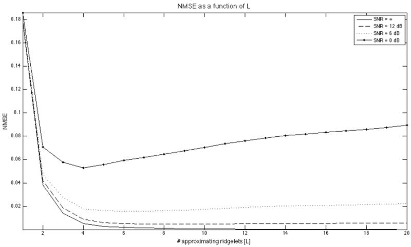
NMSE of the ridgelet approximation as a function of the number of approximating ridgelets L. The dash-dotted, dotted, dashed, and solid lines correspond to the SNR of 0, 6, 12, and ∞ dB.
Fig. 6.

(Upper panel [from left to right]) An original ODF, the corresponding diffusion directions, and the estimated ODF; (Lower panel) Approximating ridgelets.
The property of the NMSE of being a monotone decreasing function of L turns out to be relevant for the case of zero-level noise only. In the case of noisy data, the NMSE curves start exhibiting either saturation or local minima, depending on the specific level of noise. This phenomenon can be observed in Fig. 5, where the dashed, dotted, and dash-dotted curves represent the dependency of the NMSE on L for the SNR equal to 12, 6, and 0 dB, respectively.
The explanation of the above behavior of the NMSE lies in the “greedy” nature of the OMP: it tends to select ridgelets associated with the useful signal for relatively low values of L, while starting to pick out ridgelets related to noise as L keeps growing. For this reason, it was proposed in [49, Ch. 10.5] to use L as a de-noising parameter, namely to change L proportionally to the noise level so as to minimize the effect of the noise on the final approximation. Unfortunately, there does not seem to be a straightforward way to predefine an optimal L for the case when little is known about the properties of the signal to be recovered. As suggested by the simulation results (Fig. 5), however, we believe that the optimal L should be in the range between 4 and 8 depending on the specific value of SNR. We therefore proceed with our experimental study using the above values of L, while discussing some possible ways to automatically predetermine the latter in Section VII.
2) Comparison in terms of the NMSE
The results of quantitative comparison of the Fourier- and ridgelets-based methods for q-ball imaging in terms of the NMSE are summarized in Table I. For the sake of brevity, from now on we refer to these methods as FQBI and RQBI, respectively. The comparison has been performed for three different values of SNR: 12, 6, and 0 dB. The number of “fibers” in the model of (4) was defined randomly to be either 1, 2, or 3. Two different values of b, viz. 1000 and 3000 s/mm2 were used in the comparison.
TABLE I.
NMSE (±σ) of the estimation of (in silico) ODFs by means of the FQBI and RQBI methods.
| b [s/mm2] | SNR [dB] | FQBI (×10−3) m = 8, λ = 0.006 | RQBI (×10−3) |
||
|---|---|---|---|---|---|
| L = 4 | L = 6 | L = 8 | |||
| 3000 | 12 | 5.34 ± 2.33 | 8.29 ± 3.99 | 5.47 ± 2.43 | 4.73 ± 2.17 |
| 6 | 16.82 ± 9.28 | 17.84 ± 10.15 | 15.71 ± 9.01 | 16.55 ± 9.24 | |
| 0 | 63.44 ± 39.52 | 53.87 ± 34.85 | 59.63 ± 35.45 | 64.52 ± 39.36 | |
| 1000 | 12 | 0.96 ± 0.46 | 1.02 ± 0.44 | 0.88 ± 0.38 | 0.90 ± 0.41 |
| 6 | 3.87 ± 1.79 | 2.68 ± 1.23 | 2.98 ± 1.32 | 3.54 ± 1.65 | |
| 0 | 13.66 ± 6.74 | 8.59 ± 4.37 | 11.98 ± 5.24 | 13.16 ± 6.57 | |
As suggested by (4), the higher the values of b are, the broader are the spectra of corresponding HARDI signals. In particular, HARDI signals obtained for b = 1000 s/mm2 are much smoother as compared to the signals obtained using b = 3000 s/mm2. As a result, in the former case, one can estimate the corresponding ODFs with considerably smaller NMSE, as it is evident from Table 1. (It should be noted, however, that the above fact by no means suggests that one should minimize b in practical settings, since the ability of q-ball imaging to discriminate between different diffusion flows deteriorates as b becomes smaller.)
Through analyzing the results of Table 1 a few important conclusions can be made. First, as discussed above, the NMSE of RQBI depends on the number L of approximating ridgelets. Thus, for example, in the case of b = 3000 s/mm2 and SNR = 12 dB the NMSE of RQBI is minimized for L = 8, whereas the error is minimal for L = 4 when SNR approaches 0 dB. Moreover, when L is set to its optimal values (as indicated by the boldfaced entries in Table 1), RQBI outperforms FQBI in terms of the NMSE for all values of SNR. Yet even more important is the fact that when L is set non-adaptively to its “middle-range” value of L = 6, the performance of the RQBI method remains comparable with respect to (and even slightly better than) the FQBI method, while the former still has an important advantage of using 7.5 times fewer representation coefficients. To assist the reader in appreciating the noise levels used in the experiment, Fig. 7 shows an example of a HARDI signal in Subplot A along with its noisy versions in Subplots B1-B3. At the same time, Subplots C1-C3 and Subplots D1-D3 show the estimates of the original signal obtained by means of FQBI and RQBI, correspondingly.
Fig. 7.

(Subplot A) Original HARDI signal S(u) simulated with M = 3 and b = 3000 s/mm2; (Subplots B1-B3) Noisy versions of the signal corresponding to SNR = 12, 6, and 0 dB, respectively; (Subplots C1-C2) Signals estimates obtained by the FQBI method using 45 spherical harmonics; (Subplot D1-D3) Signals estimates obtained by the RQBI method using 6 spherical ridgelets.
3) Comparison in terms of the directional error
The NMSE is known to be a global performance metric. In the case of q-ball imaging, however, global errors seem to be less important as compared to the errors which occur near the maxima of ODFs. Since the latter are used for the determination of the directions of underlying diffusion flows, a reconstruction method which is capable of better preserving the directional information encoded by HARDI data should be preferred by the applications which use q-ball imaging in conjunction with fiber tractography [6, Ch.9].
To assess the directional errors of the FQBI and RQBI methods, an additional numerical experiment was carried out. In this experiment, the orientations of the local diffusion flows associated with estimated ODFs were computed using the following two-stage procedure: first, the local maxima of the ODFs were identified over the discrete grid of 321 directions vi ∈ Ω+; second, the directions of the local maxima were further refined using the steepest ascent procedure of (36). Subsequently, the directional error between the estimated and the true orientations of diffusion flows was computed according to (39). It is worthwhile noting that, in the model of (4), the (true) directions of the local diffusion flows are represented by the principal eigenvectors of the corresponding diffusion tensors Dk.
The directional errors of the FQBI and RQBI algorithms are summarized in Table II for different values of SNR. Similarly to the case of NMSE, one can see that the error of RQBI depends on L, with lower values of the latter required at lower SNR (as indicated by the boldfaced entries in the table). This dependency, however, appears to be rather mild. Moreover, the directional error of RQBI is considerably smaller than the error of FQBI for all values of L, which suggests that the basis of spherical ridgelets is more suitable for representation of directional information on Ω as compared to the basis of spherical harmonics.
TABLE II.
Directional error δ (±σ) of the ODFs estimated by means of the FQBI and RQBI methods.
| b [s/mm2] | SNR [dB] | FQBI (×10−3) m = 8, λ = 0.006 | RQBI (×10−3) |
||
|---|---|---|---|---|---|
| L = 4 | L = 6 | L = 8 | |||
| 3000 | 12 | 2.880 ± 1.400 | 2.280 ± 1.140 | 1.830 ± 0.850 | 1.670 ± 0.840 |
| 6 | 3.970 ± 1.820 | 2.920 ± 1.400 | 2.430 ± 1.170 | 2.510 ± 1.220 | |
| 0 | 6.590 ± 2.860 | 4.410 ± 2.490 | 4.450 ± 2.120 | 4.730 ± 2.120 | |
| 1000 | 12 | 6.590 ± 3.620 | 4.590 ± 2.650 | 4.410 ± 2.290 | 4.150 ± 2.040 |
| 6 | 10.470 ± 4.790 | 7.270 ± 3.500 | 7.240 ± 3.440 | 7.910 ± 3.840 | |
| 0 | 13.990 ± 7.230 | 9.230 ± 4.430 | 9.270 ± 4.370 | 10.130 ± 4.450 | |
Finally, one can see that, in the case of both algorithms, the directional errors obtained for b = 1000 s/mm2 are considerably higher than the corresponding errors obtained with b = 3000 s/mm2. This result is rooted in the fact that the spatial support of signals Sk in (4) is inversely proportional to the value of b, and hence the ability of q-ball imaging to discriminate between different diffusion directions deteriorates as b becomes smaller. Consequently, one should expect that, for certain values of the angle between crossing fibers, their orientations will be impossible to discriminate by means of the maximization procedure used in the previous experiment. In such a case, the steepest ascent will converge to a single maximum (instead of, say, two distinct ones), thereby resulting in a false detection.
The consideration above suggests that the probability of correct detection of the true number of “neural fibers” M in model (4) can serve as an additional metric to use in comparison between FQBI and RQBI. To this end, we have designed an additional experiment in which M was set to be equal to 2, while the diffusion tensors D1 and D2 were defined in such a way that the angle between their principal eigenvectors varied in the range [π/3, π/2]. Subsequently, the resulting HARDI signals were processed to recover their associated ODFs, followed by estimating the diffusion directions “encoded” by the ODFs. The case in which the number of identified (distinct) directions was equal to M = 2 was regarded as correct detection, whose probability was calculated based on the results of 1000 independent trials for both FQBI and RQBI. The resulting probabilities are shown in Fig. 8 as functions of the fiber crossing angle. The upper row of subplots in Fig. 8 represents the case of b = 3000 s/mm2 and SNR = 12, 6, and 0 dB, whereas the lower subplots were obtained for the same values of SNR and b = 1000 s/mm2. In the case of RQBI, the number of approximating ridgelets was set to be equal to L = 6. One can see that, for all the above values of SNR and b, the probabilities of correct detection by the RQBI method (solid lines) substantially exceeds the probabilities obtained using the FQBI method (dashed lines). This suggests that, as the crossing angle decreases to the point at which the modes of the ODFs become undistinguishable, RQBI is capable of correctly identifying the true number of crossing fibers in a more reliable manner as compared with FQBI. Alternatively, one can conclude that the effective resolution of RQBI is higher than that of FQBI.
Fig. 8.

(Upper row of subplots) The rates of correct detection of a two-fiber diffusion pattern by FQBI (dashed line) and RQBI (solid line) for b = 3000 s/mm2 and SNR = 12, 6, and 0 dB; (Lower row of subplots) The same as above, only with b = 1000 s/mm2.
C. Experiments with Real Data
As the next validation step, experiments with real DW-MRI data were carried out. The proposed algorithm was tested on human brain scans acquired on a 3-Tesla GE system using an echo planar imaging (EPI) diffusion-weighted image sequence. A double echo option was used to suppress eddy-current related distortions. To improve the spatial resolution of EPI, an eight channel coil was used to perform parallel imaging by means of the ASSET technique with a speed-up factor of 2. The data were acquired using 102 gradient directions (generated using the electrostatic repulsion algorithm) with b = 1000 s/mm2. In addition, eight baseline (b0) scans were acquired with b = 0. The following scan parameters were used: TR = 17000 ms, TE = 78 ms, FOV = 24 cm, 144 × 144 encoding steps, and 1.7 mm slice thickness. All scans had 85 axial slices parallel to the AC-PC line covering the whole brain.
In this section, estimated ODFs are shown superimposed over the images of their related generalized fractional anisotropy (GFA) [15]. The latter is used to quantify the degree of anisotropy of the associated diffusion flow, with its values ranging between 0 and 1, which corresponds to isotropic and maximally anisotropic flows, respectively. Specifically, the leftmost subplot of Fig. 9 demonstrates the GFA image of a coronal cross-section of the brain. The selected (rectangular) region within this image was determined according to the brain atlas [50, p. 51] to focus on the area where the fibers of corpus callosum and corona radiata are expected to intersect. The ODFs associated with the selected area, as recovered by RQBI and FQBI, are shown in Subplots A1 and B1, respectively. In the case of FQBI, the ODFs were reconstructed using m = 8 (i.e., 45 spherical harmonics), while only 6 ridgelets per ODF were used in the case of RQBI.
Fig. 9.

(Leftmost subplot) GFA image of a coronal view of the brain; (Subplot A1) RQBI-recovered ODFs corresponding to the selected area in the GFA image; (Subplot B1) FQBI-recovered ODFs corresponding to the selected area in the GFA image; (Subplots A2-A5) Examples of RQBI-recovered ODFs corresponding to the marked areas in Subplot A2; (Subplots B2-B5) Examples of FQBI-recovered ODFs corresponding to the marked areas in Subplot B2.
Taking into consideration the value of b used for data acquisition (i.e., b = 1000 s/mm2), it seems unlikely that the number of diffusion directions resolvable by q-ball imaging could be greater than 3 [51]. Thus, comparing Subplots A1 and B1 of Fig. 9 one can see that the ODFs recovered by RQBI are considerably less noisy as compared to the ODFs estimated by FQBI. Moreover, the ODFs represented by the spherical ridgelets are notably more detailed and have clearer expressed directivity as compared to the ODFs represented by the spherical harmonics. To make this conclusion more evident, Subplots A2-A5 and Subplots B2-B5 compare the ODFs corresponding to the marked voxels of Subplots A1 and B1, respectively. One can see that, while FQBI fails to resolve between different modes of the underlying diffusion flows, RQBI clearly recovers the multimodal structure of the latter. This suggests that, even thought the ridgelet representation uses considerably smaller number of approximating functions as compared with the case of spherical harmonics, it is capable of better representing the directionality of the estimated ODFs.
Finally, conclusions similar to the above can be also made observing Fig. 10, which extends the idea of Fig. 9 to a saggital cross-section of the brain. In this figure, the ODFs shown in Subplots A1 and B1 correspond to the area where callosal fibers meet with those of superior longitudinal fasciculus. Once again, the apparent gain in the separability of distinct diffusion directions (as represented by the modes of the recovered ODFs in Subplots A2-A5 and B2-B5) proves that the basis of spherical ridgelets has a superior ability to represent directional information encoded by HARDI data as compared to spherical harmonics.
Fig. 10.

(Leftmost subplot) GFA image of a sagittal view of the brain; (Subplot A1) RQBI-recovered ODFs corresponding to the selected area in the GFA image; (Subplot B1) FQBI-recovered ODFs corresponding to the selected area in the GFA image; (Subplots A2-A5) Examples of RQBI-recovered ODFs corresponding to the marked areas in Subplot A2; (Subplots B2-B5) Examples of FQBI-recovered ODFs corresponding to the marked areas in Subplot B2.
VII. Discussion and Conclusions
In this paper, we have shown conceptually and experimentally that the accuracy of reconstruction of diffusion ODFs in q-ball imaging can be considerably improved via representing the latter by means of spherical ridgelets. In particular, it has been shown that the spherical ridgelet representation allows recovering the ODFs with a lower NMSE as compared to the case of their representation by using spherical harmonics. Moreover, the ODFs recovered by the RQBI algorithm possess improved angular uncertainty (see Table II) and higher angular resolution (see Fig. 8). All these improvements appear to be particularly significant in view of the fact that RQBI uses (on average) 7.5 times fewer representation coefficients as compared to the case of FQBI. This therefore indicates that the basis of spherical ridgelets has better de-noising properties with respect to HARDI signals, and as a result it is capable of better representing the directional information encoded by the latter.
The superiority of the ridgelet representation of diffusional ODFs over their Fourier representation is rooted in the way the spherical ridgelets have been designed. In particular, they are defined to be (multiresolution) differences between scaled versions of the ridgelet generating function (RGF) – the function whose shape is highly correlated with the shape of the elementary (unimodal) signals Sk in the model (4). In this way, the resulting frame of spherical ridgelets has been adapted to represent linear combinations of such diffusion signals.
The construction of spherical ridgelets has been based on the fundamental principles of multiresolution analysis. In this respect, one should mention the recent work [52], in which HARDI signals are expanded in terms of spherical (B-spline) wavelets. While the multiresolution structure of this analysis still offers considerable improvements over the methods derived under the assumption that all Sk in (4) have the same bandwidth, the wavelets cannot provide a sparse representation of Sk. This is because the energy of the spherical wavelets is concentrated in close proximity of their center of symmetry, whereas the energy of Sk is supported alongside of the great circles. For this reason, we believe that the spherical ridgelets should be preferred over the wavelet analysis whenever sparse representation of HARDI signals and their associated ODFs is required.
In the present paper, the ridgelet representations of diffusional ODFs were computed by means of the orthogonal matching pursuit (OMP) algorithm, which has been chosen primarily because of its property of being numerically efficient. This algorithm (also known to statisticians as stepwise regression [53]) is known to be effective in empirical works. For the reason of space, however, the present paper does not provide a theoretical analysis of the convergence properties of the OMP algorithm in the case of sparse approximation of diffusional ODFs. Thus, if the OMP method is to be used in future applications of RQBI, such an analysis (which could be based, e.g., on the results of [48], [54]) should be reported. Deriving such theoretical results is among the objectives of our current research.
It should be noted that in the case when the OMP algorithm is used for sparse approximation, the cardinality L of the approximating set is used akin to a regularization parameter, which generally depends on SNR. Setting an appropriate L seems to be a problem on its own, which might be seen as a disadvantage of the approach. It should be noted, however, that recent advances in the theory of sparse approximation offer a number of alternative algorithms which do not require knowing the number of approximating ridgelets in advance. Thus, for example, iterative thresholding [55], [56] is currently regarded as a computationally efficient procedure for computing the sparse approximations of noisy signals. A thorough overview of a number of similar methods can be found in [57]. Needless to say, all such methods can be potentially used (instead of the OMP) to solve the problem at hand.
The spherical ridgelets can be considered to be the images of spherical wavelets under the Funk-Radon transform. Specifically, the wavelets used in the present paper are the Gauss-Weiersrass M-scale wavelets [29]. Obviously, the above choice of the wavelet functions is not unique, and therefore the performance of RQBI can be further optimized over different wavelet bases. Moreover, the frame of spherical ridgelets as defined by (27) is parameterized by the scaling parameter ρ. It is important to understand that the frame is capable of stably representing the HARDI signals for any value of this parameter. However, in the case when the number of approximating ridgelets is fixed, one could argue that some values of ρ could “work better” than others. Such an optimal value of ρ could be further found using, for instance, a version of the iterative procedure in [58]. In this case, an initial value of ρ (e.g., ρ = 0.5) could be used to compute the sparse approximations of a number of HARDI signals, followed by updating ρ to be equal to a minimizer of a discrepancy measure between the approximated and measured signals. Subsequently, the above steps (i.e., the approximation and update) could be repeated iteratively until convergence of ρ to its optimal value.
Although it was shown via numerical simulations that the effective resolution of RQBI is superior to that of FQBI (in the sense of Fig. 8), neither of the two methods can improve the resolution of q-ball imaging above its intrinsic limit (as defined by the diffusivity of brain tissue as well as by the parameters of diffusion gradients). In order to extend the resolution limit, spherical deconvolution needs to be performed [17], [24]-[26]. Because of the ill-posed nature of the deconvolution as an inverse problem, its performance heavily depends on the accuracy with which the diffusion ODFs can be recovered. The fact that RQBI outperforms FQBI in terms of both global (NMSE) and local (directional) errors suggests that RQBI can provide a better input to deconvolution, thereby improving its overall performance. As a result, we expect that using the deconvolution in conjunction with RQBI can could be used as an important preprocessing stage for fiber tractography. Verifying this assumption forms another important direction of our current research.
Acknowledgments
The authors are grateful to all the anonymous reviewers, whose valuable remarks, comments, and suggestions have allowed the authors to substantially improve the quality of this manuscript. The authors would also like to thank Dr. James Malcolm for his invaluable input and help with the visualization of some results presented in this paper.
This research was supported by a Discovery grant from NSERC – The Natural Sciences and Engineering Research Council of Canada. Information on various NSERC activities and programs can be obtained from http://www.nserc.ca.
Footnotes
The approximation of ODFs in [22] uses 45 spherical harmonics.
In general, the sums in (4) should be multiplied by the the so-called “b0 image” S0 (u) which we assume to be equal to 1 without any loss of generality.
Without any loss of generality, one can set v0 = [0, 0, 1]T, so that both K0 (·v0) and Wj (·v0) are always oriented along the z-axis in ℝ3.
The fractional anisotropy (FA) index corresponding to the tensor is equal to 0.8
Contributor Information
Oleg Michailovich, School of Electrical and Computer Engineering, University of Waterloo, Canada N2L 3G1 (phone: 519-888-4567 (ext. 38247); olegm@uwaterloo.ca).
Yogesh Rathi, Psychiatry Neuroimaging Laboratory (Department of Psychiatry, Brigham and Women’s Hospital, Harvard Medical School), Boston, MA 02115 USA, yogesh@bwh.harvard.edu.
Martha E. Shenton, Psychiatry Neuroimaging Laboratory (Department of Psychiatry, Brigham and Women’s Hospital, Harvard Medical School), Boston, MA 02115 USA, shenton@bwh.harvard.edu
References
- 1.LeBihan D, Breton E, Lallemand D, Grenier P, Cabanis E, Laval-Jeantet M. MR imaging of intravoxel incoherent motions: Application to diffusion and perfusion in neurological disorders. Radiology. 1986 Nov;161:401–407. doi: 10.1148/radiology.161.2.3763909. [DOI] [PubMed] [Google Scholar]
- 2.Basser PJ, Mattiello J, LeBihan D. Estimation of the effective self-diffusion tensor from the NMR spin echo. J Magn Reson Imag B. 1994 Mar;103(no. 3):247–254. doi: 10.1006/jmrb.1994.1037. [DOI] [PubMed] [Google Scholar]
- 3.Basser PJ, Pajevic S, Pierpaoli C, Duda J, Aldroubi A. In vivo fiber tractography using DT-MRI data. Magn Reson Med. 2000;44:625–632. doi: 10.1002/1522-2594(200010)44:4<625::aid-mrm17>3.0.co;2-o. [DOI] [PubMed] [Google Scholar]
- 4.Campbell J, Siddiqi K, Rymar VV, Sadikot AF, Pike GB. Flow-based fiber tracking with diffusion tensor and q-ball data: Validation and comparison to principal diffusion direction techniques. NeuroImage. 2005;27:725–736. doi: 10.1016/j.neuroimage.2005.05.014. [DOI] [PubMed] [Google Scholar]
- 5.Bihan DL, Mangin J-F, Poupon C, Clark C, Pappata S, Molko N, Chabriat H. Diffusion tensor imaging: Concepts and applications. J Magn Reson Imag. 2001;13:534–546. doi: 10.1002/jmri.1076. [DOI] [PubMed] [Google Scholar]
- 6.Mori S. Introduction to Diffusion-Tensor Imaging. Elsevier; 2007. [Google Scholar]
- 7.Wiegell MR, Larsson H, Wedeen VJ. Fiber crossing in human brain depicted with diffusion tensor MR imaging. Radiology. 2000;217:897–903. doi: 10.1148/radiology.217.3.r00nv43897. [DOI] [PubMed] [Google Scholar]
- 8.Alexander DC, Barker GJ, Arridge SR. Detection and modeling of non-Gaussian apparent diffusion coefficient profiles in human brain data. J Magn Reson Med. 2002;48(no. 2):331–340. doi: 10.1002/mrm.10209. [DOI] [PubMed] [Google Scholar]
- 9.Frank LR. Characterization of anisotropy in high angular resolution diffusion-weighted MRI. Magn Reson Med. 2002;47:1083–1099. doi: 10.1002/mrm.10156. [DOI] [PubMed] [Google Scholar]
- 10.Anderson AW. Measurement of fiber orientation distributions using high angular resolution diffusion imaging. Magn Reson Med. 2005;54:1194–1206. doi: 10.1002/mrm.20667. [DOI] [PubMed] [Google Scholar]
- 11.Descoteaux M, Angelino E, Fitzgibbons S, Deriche R. Apparent diffusion coefficients from high angular resolution diffusion images: Estimation and applications. Magn Reson Med. 2006;56(no. 2):395–410. doi: 10.1002/mrm.20948. [DOI] [PubMed] [Google Scholar]
- 12.Hess CP, Mukherjee P, Han ET, Xu D, Vigneron DR. Q-ball reconstruction of multimodal fiber orientations using the spherical harmonic basis. Magn Reson Med. 2006;56:104–117. doi: 10.1002/mrm.20931. [DOI] [PubMed] [Google Scholar]
- 13.Tuch DS, Reese TG, Wiegell MR, Makris N, Belliveau JW, Wedeen VJ. High angular resolution diffusion imaging reveals intravoxel white matter fiber heterogeneity. Magn Reson Med. 2002;48:577–582. doi: 10.1002/mrm.10268. [DOI] [PubMed] [Google Scholar]
- 14.Tuch DS, Reese TG, Wiegell MR, Wedeen VJ. Diffusion MRI of complex neural architecture. Neuron. 2003;40:885–895. doi: 10.1016/s0896-6273(03)00758-x. [DOI] [PubMed] [Google Scholar]
- 15.Tuch DS. Q-ball imaging. Magn Reson Med. 2004;52:1358–1372. doi: 10.1002/mrm.20279. [DOI] [PubMed] [Google Scholar]
- 16.Helgason S. The Radon transform. 2. Birkhäuser; 1999. [Google Scholar]
- 17.Alexander DC. Multiple-fiber reconstruction algorithms for diffusion MRI. Ann NY Acad Sci. 2005;1064:113–133. doi: 10.1196/annals.1340.018. [DOI] [PubMed] [Google Scholar]
- 18.Kreher BW, Schneider JF, Mader I, Martin E, Hennig J, Ilyasov KA. Multi-tensor approach for analysis and tracking of complex fiber configurations. Magn Reson Med. 2005;54:1216–1225. doi: 10.1002/mrm.20670. [DOI] [PubMed] [Google Scholar]
- 19.McGraw T, Vemuri B, Yezierski B, Mareci T. Proc of ISBI. Arlington, VA: Apr, 2006. Von Mises-Fisher mixture model of the diffusion ODF. [DOI] [PMC free article] [PubMed] [Google Scholar]
- 20.Schultz T, Seidel H. Estimating crossing fibers: A tensor decomposition approach. IEEE Trans Visual Comput Graphics. 2008;14(no. 6):1635–1642. doi: 10.1109/TVCG.2008.128. [DOI] [PubMed] [Google Scholar]
- 21.Rathi Y, Michailovich O, Shenton ME, Bouix S. Directional functions for orientation distribution estimation. Med Image Anal. 2009 June;13(no. 3):432–444. doi: 10.1016/j.media.2009.01.004. [DOI] [PMC free article] [PubMed] [Google Scholar]
- 22.Descoteaux M, Angelino E, Fitzgibbons S, Deriche R. Regularized, fast, and robust analytical Q-ball imaging. 2007;(no. 58):497–510. doi: 10.1002/mrm.21277. [DOI] [PubMed] [Google Scholar]
- 23.Tournier J-D, Calamante F, Gadian DG, Connelly A. Direct estimation of the fiber orientation density function from diffusion-weighted MRI data using spherical deconvolution. NeuroImage. 2004;23:1176–1185. doi: 10.1016/j.neuroimage.2004.07.037. [DOI] [PubMed] [Google Scholar]
- 24.Jansons KM, Alexander DC. Persistent angular structure: New insights from diffusion magnetic resonance imaging data. Inverse Problems. 2003;19:1031–1046. [Google Scholar]
- 25.Jian B, Vemuri BC. A unified computational framework for deconvolution to reconstruct multiple fibers from diffusion weighted MRI. IEEE Trans Med Imag. 2007 Nov;26(no. 11):1464–1471. doi: 10.1109/TMI.2007.907552. [DOI] [PMC free article] [PubMed] [Google Scholar]
- 26.Sakaie KE, Lowe MJ. An objective method for regularization of fiber orientation distributions derived from diffusion-weighted MRI. NeuroImage. 2007;34:169–176. doi: 10.1016/j.neuroimage.2006.08.034. [DOI] [PubMed] [Google Scholar]
- 27.Verma R, Khurd P, Davatzikos C. On analyzing diffusion tensor images by identifying manifold structure using isomaps. IEEE Trans Med Imag. 2007 June;26(no. 6):772–778. doi: 10.1109/TMI.2006.891484. [DOI] [PubMed] [Google Scholar]
- 28.Descoteaux M, Deriche R. High angular resolution diffusion MRI segmentation using region-based statistical surface evolution. J Math Imaging Vis. 2009 Feb;33(no. 2):239–252. [Google Scholar]
- 29.Freeden W, Schreiner F. Orthogonal and non-orthogonal multiresolution analysis, scale discrete and exact fully discrete wavelet transform on the sphere. Constr Approx. 1998;14:493–515. [Google Scholar]
- 30.Antoine J-P, Demanet L, Jacques L, Vandergheynst P. Wavelets on the sphere: implementation and approximations. Appl Comput Harmon Anal. 2002;13(no. 3):177–200. [Google Scholar]
- 31.McEwen JD, Hobson MP, Mortlock DJ, Lasenby AN. Fast directional continuous spherical wavelet transform algorithms. IEEE Trans Signal Processing. 2007;55(no. 2):520–529. [Google Scholar]
- 32.Freeden W, Schreiner M. Spherical Functions of Mathematical Geosciences: A Scalar, Vectorial, and Tensorial Setup. Springer-Verlag; 2008. [Google Scholar]
- 33.Candes EJ, Donoho DL. Ridgelets: A key to high-dimentional intermittency? Phil Trans R Soc Lond. 1999;357:2495–2509. [Google Scholar]
- 34.Pati Y, Rezaiifar R, Krishnaprasad P. Orthogonal matching pursuit: recursive function approximation with applications to wavelet decomposition. Proc the 27th Annual Asilomar Conference on Signals, Systems, and Computers. 1993 Nov; [Google Scholar]
- 35.Starck J-L, Moudden Y, Abrial P, Nguyen M. Wavelets, ridgelets and curvelets on the sphere. Astronomy and Astrophysics. 2006;446:1191–1204. [Google Scholar]
- 36.Rubin B. Spherical Radon transform and related wavelet transforms. Appl Comput Harm Anal. 1998;5:202–215. [Google Scholar]
- 37.Michailovich O, Rathi Y. Proc of ISBI. Paris: 2008. Approximation of orientation distribution functions by spherical ridgelets. [DOI] [PMC free article] [PubMed] [Google Scholar]
- 38.Hobson EW. The theory of spherical and ellipsoidal harmonics. Chelsea Publishing Company; 1955. [Google Scholar]
- 39.Groemer H. Geometric applications of Fourier series and spherical harmonics. Cambridge University Press; 1996. [Google Scholar]
- 40.Freeden W, Schreiner M, Franke R. A survey on spherical spline approximation. Surv Math Ind. 1997;7:29–85. [Google Scholar]
- 41.Bogdanova I, Vandergheynst P, Antoineb J-P, Jacquesb L, Morvidoneb M. Stereographic wavelet frames on the sphere. Applied Comput Harm Anal. 2005;19(no. 2):223–252. [Google Scholar]
- 42.Rao BD, Kreutz-Delgado K. An affine scaling methodology for best basis selection. IEEE Trans Signal Processing. 1999 Jan;47(no. 1):187–200. [Google Scholar]
- 43.Chen SS, Donoho DL, Saunders MA. Atomic decomposition by basis pursuit. SIAM Review. 2001;43(no. 1):129–159. [Google Scholar]
- 44.Tropp JA, Gilbert AC. Signal recovery from random measurements via orthogonal matching pursuit. IEEE Trans Inform Theory. 2007 Dec;53(no. 12):4655–4666. [Google Scholar]
- 45.Driscoll JR, Healy DM. Computing Fourier transforms and convolutions on the 2-sphere. Adv Appl Math. 1994;15:202–250. [Google Scholar]
- 46.Strang G. Introduction to applied mathematics. Wellesley, MA: Wellesley-Cambridge Press; 1986. [Google Scholar]
- 47.Fiori S. Geodesic-based and projection-based neural blind deconvolution algorithms. Signal Process. 2008 Mar;88(no. 3):521–538. [Google Scholar]
- 48.Temlyakov VN. Greedy algorithms and M-term approximation with regard to redundant dictionaries. J Approx Theory. 1999 May;99(no. 1):117–145. [Google Scholar]
- 49.Mallat S. A wavelet tour of signal processing. 2. Academic Press; 1999. [Google Scholar]
- 50.Woolsey TA, Hanaway J, Gado MH. The brain atlas: A visual guide to the human nervous system. 3. Hoboken, NJ: John Wiley and Sons Inc; 2008. [Google Scholar]
- 51.Behrens T, Johansen-Berg H, Jbabdi S, Rushworth M, Woolrich M. Probabilistic diffusion tractography with multiple fiber orientations: What can we gain? NeuroImage. 2007;34:144–155. doi: 10.1016/j.neuroimage.2006.09.018. [DOI] [PMC free article] [PubMed] [Google Scholar]
- 52.Kezele I, Descoteaux M, Poupon C, Abrial P, Poupon F, Mangin J-F. Proceedings of the Workshop on Comput Diffus MRI, MICCAI. New York NY, USA: Sept, 2008. Multiresolution decomposition of HARDI and ODF profiles using spherical wavelets. [Google Scholar]
- 53.Draper N, Smith H. Applied regression analysis. 2. New York: John Wiley and Sons; 1981. [Google Scholar]
- 54.Tropp JA. Greed is good: Algorithmic results for sparse approximation. IEEE Trans Inform Theory. 2004 Oct;50(no. 10):2231–2242. [Google Scholar]
- 55.Daubechies I, Defrise M, DeMol C. An iterative thresholding algorithm for linear inverse problems with a sparsity constraint. arXiv:math/0307152v2. 2003 [Google Scholar]
- 56.Blumensath T, Davies ME. Iterative thresholding for sparse approximations. J Fourier Anal Appl. 2008 Dec;14(no. 5-6):629–654. [Google Scholar]
- 57.Elad M, Matalon B, Shtok J, Zibulevsky M. Proceedings of SPIE (Wavelet XII) San-Diego CA, USA: 2007. A wide-angle view at iterated shrinkage algorithms. [Google Scholar]
- 58.Aharon M, Elad M, Bruckstein A. K-SVD: An algorithm for designing overcomplete dictionaries for sparse representation. IEEE Trans Signal Processing. 2006 Nov;54(no. 11):4311–4322. [Google Scholar]