Multi-Shot 3D Slice-Select Tailored RF Pulses for MRI

Abstract

A multi-shot three-dimensional slice-select tailored RF pulse method is presented for the excitation of slice profiles with arbitrary resolution. This method is derived from the linearity of the small tip angle approximation, allowing for the decomposition of small tip angle tailored RF pulses into separate excitations. The final image is created by complex summation of the images acquired from the individual excitations. This technique overcomes the limitation of requiring long pulse to excite thin slices with adequate resolution. This has implications in applications including T2*-weighted functional MRI in brain regions corrupted by intravoxel dephasing artifacts due to susceptibility variations. Simulations, phantom experiments, and human brain images are presented. It is demonstrated that at most four shots of 40 ms pulse length are needed to excite a 5 mm thick slice in the brain with reduced susceptibility artifacts at 3T.

INTRODUCTION

Rapid imaging methods such as spiral imaging (1-3) or echo planar imaging (4,5) are of current interest in MRI. These methods are widely implemented in brain functional MRI (fMRI) due to their high sensitivity to blood oxygen level dependent (BOLD) T2* contrast (6,7) and due to their high temporal and spatial resolution of brain activity. However, the long echo times required for BOLD T2* contrast make the images acquired with these modalities more prone to intravoxel dephasing from magnetic susceptibility variations near air/tissue boundaries. Susceptibility artifacts in BOLD fMRI plague many brain regions that are significant for psychiatric and basic neuroscientific research, including the orbitalfrontal and inferior and medial temporal cortices. Therefore, the development of methods which can reduce susceptibility artifacts and still preserve sensitivity to BOLD T2* contrast with high temporal and spatial resolution is of importance.

Numerous methods have been proposed to mitigate susceptibility artifacts in T2* weighted imaging, including automatic shimming (8), data post processing (9-12), gradient compensation (13-18), thin slice averaging (19-21), and tailored RF pulses (22-25). Specifically, three-dimensional slice-select tailored RF (3D SSTRF) pulses (23,25) are a promising technique due to their potential for the correction of intravoxel dephasing artifacts in specific anatomical regions leaving the rest of the image unaffected. Recent work by our group demonstrated that 3D SSTRF pulses are capable of acquiring a 1-2 cm thick slice with reduced susceptibility artifacts in one shot at 3T using spatial saturation pulses to suppress sidelobes. However, the excitation of a 3-5 mm thick slice with no spatial saturation would require a pulse approximately 120-160 ms in length for adequate sampling resolution given the hardware requirements of conventional body scanners. Not only are long pulses impractical, they are also more prone to off-resonance shifts of the slice profile and will have a spatial varying TE.

This paper presents a multi-shot 3D SSTRF approach to overcome the penalty of long pulse lengths needed for high-resolution 3D slice profiles. This method exploits the linearity of the small tip angle approximation (26) by breaking up the pulses into orthogonal components that excite the slice in separate acquisitions. The final image is obtained by summation of the complex image data. Although work has been done demonstrating the utility of multi-shot methods for 2D tailored RF small-tip pulses (27,28), no work has demonstrated a method for multi-shot 3D SSTRF pulses. Furthermore, there has been no work demonstrating its use for the reduction of intravoxel dephasing artifacts in T2* weighted imaging applications. This work proposes that multi-shot 3D SSTRF pulses can be designed using interleaved stacked spiral k-space trajectories. Simulations, phantom imaging experiments, and human brain images are presented which demonstrate the methodology.

THEORY

Within the small tip angle approximation, theoretically valid for tip angles less than 30° but shown to hold well for angles up to 90°, the RF field B₁(t) as a function of time t can be written

$$B_1(t)\propto \mathrm{\Delta }(\mathbf{k}(t))\left|\mathbf{G}(t)\right|\left\{\int M_{\mathit{xy}}(\mathbf{r})e^{i\mathbf{k}(t)·\mathbf{r}}d\mathbf{r}\right\},\mathrm{where}\mathbf{k}(t)=-\gamma {\int }_t^T\mathbf{G}(s)\mathit{ds}.$$ [1]

In the above equations Δ(k(t)) is a sample density correction term (29), G(t) are the gradients that are applied simultaneously to B₁(t), and M_xy(r) is the desired complex transverse magnetization. The k-space vector k(t) is determined by the area remaining under the gradients between t and the end of the pulse (of pulse width T). Any arbitrary analytical or numerical form for M_xy(r) can be used as long as the sampling requirements are satisfied for the resolution of M_xy(r) and for the 3D FOV of the area being imaged. For example, the analytical form of an azimuthally symmetric disk of magnetization can be created for M_xy(r) in cylindrical coordinates using a circ function for the x-y direction multiplied by a Gaussian for the z direction:

$$M_{\mathit{xy}}(\rho ,z)=\exp \left[-\pi {(z/z_0)}^2\right]\mathrm{circ}(\rho /{\rho }_0).$$ [2]

Here z₀ is the slice thickness and ρ₀ is in-plane radius of the disk. The function circ(ρ/ρ₀) is defined as being 0 when ρ > ρ₀ and 1 when ρ ≤ ρ₀.

Compensation for the signal loss artifact due field inhomogeneity from susceptibility variations can be accomplished by adding a phase term to M_xy(r) which is equal but opposite in sign of the phase accrued at TE due to inhomogeneity:

$$M_{\mathit{xy}}(\mathbf{r},\mathit{TE})=M_{\mathit{xy}}(\mathbf{r},0)\exp [-i\omega (\mathbf{r})\mathit{TE}].$$ [3]

In this equation ω(r) is the spatially dependent rate of phase change. The echo time TE is defined as the time between when the center of k-space is excited (approximately the center of the RF pulse) and when the center of k-space is acquired. Equation [3] assumes that the shifts in time along the RF produced by the phase term are small compared to TE. In many brain regions, such as above the sagittal sinus, the dominant contribution to ω(r) will be linear along the z-axis (or the through-plane direction for an axial slice). For convenience, one can approximate a slice with a localized, linear through-plane phase using a summation of disks with analytical Fourier transforms (25). The Fourier transform of a representative disk can be expressed in cylindrical coordinates as the product of a Gaussian and a first-order Bessel function:

$$m_{\mathit{xy}}^{{\rho }_0{z}_0}(k_{\rho },k_z)=2\pi z_0{\rho }_0^2\exp \left[-\frac{{\left(k_z{z}_0\right)}^2}{4\pi }\right]\frac{J_1\left(k_{\rho }{\rho }_0\right)}{k_{\rho }{\rho }_0}$$ [4]

The location and the through-plane phase of the disk can be manipulated by adding a phase factor and a shift to Eq. [4], respectively. For example, a slice that reduces signal loss above a specific anatomical location, such as the sinus, would require a through-plane phase correction in the region above the sinus. This can be approximated by the summation of three disks:

$$m_{\mathit{xy}}=m_{\mathit{xy}}^{\mathit{ab}}(k_{\rho },k_z)-m_{\mathit{xy}}^{\mathit{cb}}(k_{\rho },k_z)e^{{\mathit{ik}}_{y}d}+m_{\mathit{xy}}^{\mathit{cb}}(k_{\rho },k_z+\mathrm{\Delta }{k}_z)e^{{\mathit{ik}}_{y}d}.$$ [5]

This equation represents the Fourier transform of a magnetization profile for a 3D slice with an in-plane radius a, thickness b, and a through-plane phase correction of radius c located a distance d posterior from the center of the slice. The magnitude of the through-plane phase correction term is proportional to the shift Δk_z of the small disk. Although the use of an in-vivo anatomical map of the desired magnetization profile is possible with the 3D SSTRF method, approximate analytical functions ease implementation and are adequate for demonstration purposes.

In practice, the sampling time of the 3D SSTRF pulse is finite and discrete such that the there is a minimum resolution and maximum FOV over the volume excited by the pulse. The resolution determines how well defined the slice will be and how fine the variations in magnitude and phase will be through its volume. The FOV will determine the locations of the aliases (sidelobes) of the slice volume. The long lengths required for 3D SSTRF pulses with high resolutions and large FOV’s are the primary drawback of the method. For example, to reduce intravoxel dephasing artifacts in T2* weighted imaging, pulses on the order of 120-160 ms are needed to excite a 5 mm thick slice with a 20 cm FOV in all three dimensions and a volumetric resolution of 1.5×1.5×0.1 cm (x, y, and z respectively). Not only are long pulses impractical due to the long minimum TE, they are also more prone to off-resonance slice shifts and have spatially dependent echo times.

To overcome the limitation of long pulse lengths, due to the linearity of the small tip angle approximation, the 3D SSTRF pulses can be subdivided into shots that are applied as separate excitations and acquisitions. The final image excited by the 3D SSTRF pulses is obtained by summing the complex image data. An efficient k-space trajectory choice for the 3D SSTRF pulses uses stacked spirals (30,31). Two possible multi-shot 3D SSTRF k-space trajectories using stacked spirals are an interleaved spiral (“pinwheel”) design and a design that skips spirals along k_z (“skip-k_z”). The choice of trajectory determines where aliases will appear and has an impact on pulse length and the ability to do multi-slice imaging. Figure 1 shows diagrams of the pinwheel (top) and skip-k_z (bottom) 3D SSTRF k-space trajectories. The solid and dotted lines refer to trajectories from different shots. Figure 2 shows diagrams of multi-shot 3D SSTRF pulses using the pinwheel (top) and skip-k_z (bottom) designs. These diagrams show one typical shot from four-shot pulses that were designed for use in the phantom imaging experiment described below. These pulses are qualitatively similar to all of the pulses described in this work. The rows from top to bottom show the real part of the RF, the imaginary part of the RF, the x gradient, y gradient, and z gradient. The stacked spiral trajectory is formed from the x-y gradients that generate alternating in-out spirals and from the blips generated by z gradients. Note that the pinwheel pulse has more z blips and shorter length spirals compared to the skip-k_z pulse.

Figure 1.

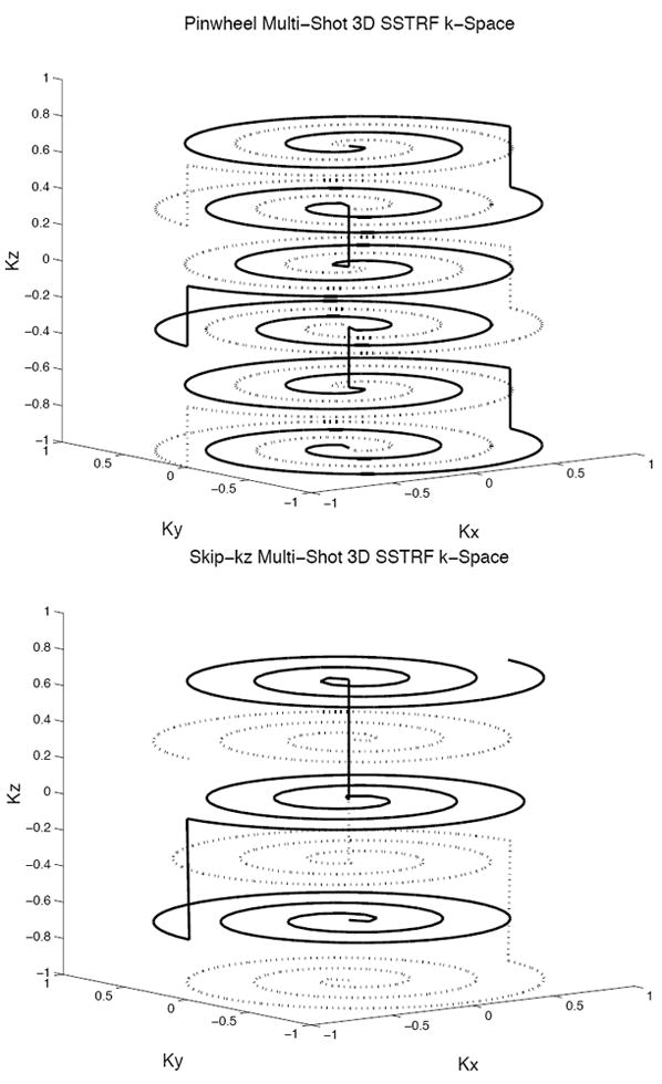
Diagrams of the k-space trajectories used for the pinwheel (top) and skip-k_z (bottom) multi-shot 3D SSTRF pulse designs. The solid and dotted lines represent two different shots.

Figure 2.

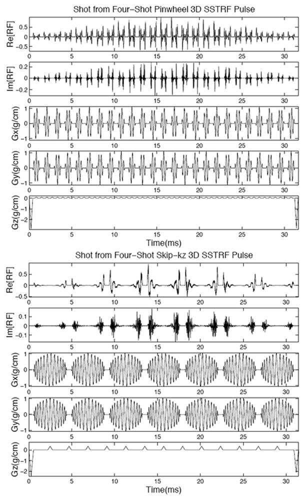
Diagrams of multi-shot 3D SSTRF pulses using the pinwheel (top) and skip-k_z (bottom) designs. These diagrams show one shot from a four-shot pulse that excites a 2 cm thick slice with a 20 cm 3D FOV. The volumetric resolution of the pulse was 5 mm for both the in-plane through-plane directions. The rows from top to bottom show the real and imaginary part of the RF and the x, y, and z gradients. These pulses produced the phantom images with the writing “3D SSTRF” shown in Fig. 5.

METHODS

The multi-shot 3D SSTRF pulses were designed for implementation on a 3T GE LX scanner running under the 8.2.5 software version (General Electric Medical Systems, Milwaukee, Wisconsin). The gradient slew rate was 150 T/m/sec and the peak gradient amplitude was 40 mT/m. The gradient waveforms for the spiral trajectories were generated analytically (32) and each successive in-out pair in the pulse were rotated 90° to reduce the sidelobes in the x-y plane. The sample-density correction term Δ(k(t)) in Eq. [1] was approximated using the method described in Reference (2). The area of each z blip determined the FOV along the slice select direction. The FOV along all of the three dimensions was fixed at 20 cm, sufficient to place all of the sidelobes outside of either an 18 cm diameter silicone phantom or a typical human head. The resolution of the pulse in the x-y plane and the z-direction, the slice thickness, and the in-plane radius varied depending on the application as did the use of Equations 2 and 5 which were used to tailor the slice volume. Although there is no theoretical limit on the maximum obtainable resolution of the 3D SSTRF excitation, restrictions in the available waveform memory forced a practical limitation of four shots, each with five individual waveforms of 40 ms each length (10,000 points stored as short integers with a 4 μs dwell time). Redundancy in the x, y and z gradients for the different shots was exploited to reduce the demand on the available memory. The flip angle of the 3D SSTRF pulses was defined by scaling the area of the magnitude of the RF to the standard sinc pulse used in the prescan procedures. The 3D SSTRF pulses were generated off-line using Matlab (The MathWorks, Inc., Natick, MA) and inserted into a standard spiral pulse sequence used for routine T2* weighted applications such as fMRI.

Numerical simulations of the 3D Bloch equations were performed to observe the structure and cancellations of the sidelobes. Four-shout pinwheel and skip-k_z 3D SSTRF pulses were designed that excited a transverse magnetization of the form described by Eq. [2]. The final FOV (resolution) of the multi-shot pulses was approximately 20 (1.5) cm in x-y and 10 (0.5) cm in z, the slice thickness z₀ was equal to 1 cm, and the in-plane radius ρ₀ was equal to 9 cm. Flip angles of 45° and 90° were used. Each shot was used as input in a 3D Bloch equation simulation. The final composite image was formed by complex summation of the transverse magnetization produced by all four shots from each pulse. Experiments were also performed on a silicone gel phantom 18 cm in diameter. Four-shot pinwheel and skip-k_z 3D SSTRF pulses were designed that excited a transverse magnetization of the form described by Eq. [2] with the addition of a numerical masking function that produced the writing “3D SSTRF” in the excited magnetization profile. The final FOV (resolution) of the multi-shot pulses used in the phantom experiments was approximately 20 (0.5) cm in x-y and 20 (0.5) cm in z, the slice thickness z₀ was equal to 2 cm, and in-plane radius ρ₀ was equal to 9 cm. The length of each pulse was approximately 40 ms, TE was equal to 20 ms, and a flip angle of 45° was used.

Finally, human brain images were acquired to test the method in-vivo. A four-shot skip-k_z 3D SSTRF pulse was designed using Eq. [5] that that would excite a 5 mm thick axial slice above the sinus at 3T. The FOV (resolution) of the pulse was 20 (1.2) cm in x-y and 20 (0.1) cm in z, z₀ = 5 mm, and ρ₀ = 9 cm. The length of each shot of the pulse was approximately 40 ms such that the minimum TE was 20 ms, a reasonable echo time for a T2* weighted fMRI acquisition at 3T. The TR of the acquisition was 1 sec and a flip angle of 60° was determined from calculating the Ernst angle. The procedure was to first acquire a sagittal scout to position the 3D SSTRF axial slice. The axial slice was acquired using the 3D STTRF pulse without and with the phase correction. The magnitude and location of the phase correction in Eq. [5] was determined by inspection of the resultant images. The smaller phase correction disk was first placed in the center of the slice and gradually moved posterior until it was positioned over the sinus artifact. The amount of through-plane phase (shift along k_z of the smaller disk) and extent was adjusted until signal was recovered in the sinus. A two-shot spiral was used for the acquisition of a 64×64 matrix to minimize the effects of in-plane susceptibility-induced inhomogeneity. Four normal human volunteers were studied.

RESULTS

Figures 3 and 4 show mesh plots displaying the results of the simulation experiments. Figure 3 shows the transverse component of the magnetization M_xy as a function of x and z excited by the four-shot pinwheel 3D SSTRF pulse with a 45° flip angle. The top eight small mesh plots show the individual real (left) and imaginary (right) parts of M_xy excited by each shot, shown from top to bottom. The bottom large mesh plot shows the magnitude of M_xy produce after the complex summation of all of the shots. The boundaries of the mesh plots along x-z are equal to the FOV of the composite pulse. The final slice has no sidelobes within the excitation FOV of the pulse. It can also be seen from the top eight plots in Fig. 3 that radial sidelobes appear distributed along the slice-select or z-direction as a result of the undersampled in-plane magnetization. The z-dependence of the radial sidelobes results from an effective undersampling along z due to the rotations of the spirals in the pulse design. Figure 4 is similar to Fig. 3 except in this figure the skip-k_z pulse was used as input. It can be seen from the top eight small mesh plots in Fig. 4 that the sidelobes appear as replications of the desired central slice along the slice-select or z-direction. The final slice has no sidelobes within the excitation FOV of the pulse. The simulations using the 90° flip-angle pulses showed qualitatively the same slice profiles and cancellations of sidelobes.

Figure 3.

Mesh plots of the transverse component of the magnetization M_xy as a function of x and z excited by a four-shot pinwheel 3D SSTRF RF pulse produced by numerical simulation of the Bloch equations. The top eight diagrams show the individual real (left) and imaginary (right) parts of M_xy excited by each shot (top to bottom). The bottom mesh plot shows the magnitude of M_xy produce after the complex summation of all of the shots.

Figure 4.

Mesh plots of the transverse component of the magnetization M_xy as a function of x and z excited by a four-shot skip-k_z 3D SSTRF RF pulse produced by numerical simulation of the Bloch equations. The top eight diagrams show the individual real (left) and imaginary (right) parts of M_xy excited by each shot (top to bottom). The bottom mesh plot shows the magnitude of M_xy produce after the complex summation of all of the shots.

Figure 5 shows the results of the phantom imaging experiments where images were acquired with the writing “3D SSTRF” excited in the slice using the pulses shown in Fig. 2. Figure 5 (a) and (b) show images of the x-z plane of the phantom from one and all four shots of the pinwheel pulse. Note that the sidelobe structure is similar to what was seen in the simulations shown in Fig. 3. Figure 5 (c) and (d) show images of the x-y plane of the phantom from one and all four shots of the pinwheel pulse. The writing “3D SSTRF” is clearly seen in the slice shown by Fig. 5 (d). Similarly, Figure 5 (e) and (f) show images of the x-z plane of the phantom from one and all four shots of the skip-k_z pulse. These images are similar to the simulations shown in Fig. 4 with regards to the distribution of sidelobes. Figure 5 (g) and (h) show images of the x-y plane of the phantom from one and all four shots of the skip-k_z pulse. Again, the writing “3D SSTRF” is clear in the slice. Figure 6 shows plots of the magnitude profiles along the slice-select direction from the phantom images. This profile is indicated by the dotted lines in Figure 5 (a) and (b) and (e) and (f). The top figure shows the profile from the images produced using the four-shot pinwheel 3D SSTRF pulse. The dashed and solid lines represent the profiles produced from one shot and from all four shots, respectively. Similarly, the bottom figure shows the profile from the images produced using the four-shot skip-k_z 3D SSTRF pulse. The residual signal from the cancelled sidelobes is 2-3% of the magnitude of the central slice.

Figure 5.

Phantom images with the writing “3D SSTRF” excited in the slice obtained using the pulses shown in Fig. 2. Images (a) and (b) show the x-z plane of the phantom from one and all four shots of the pinwheel pulse. Images (c) and (d) show the x-y plane of the phantom from one and all four shots of the pinwheel pulse. Images (e) and (f) show the x-z plane of the phantom from one and all four shots of the skip-k_z pulse. Images (g) and (h) show the x-y plane of the phantom from one and all four shots of the skip-k_z pulse. The dotted lines indicate the locations of the profile plots shown in Fig. 6.

Figure 6.

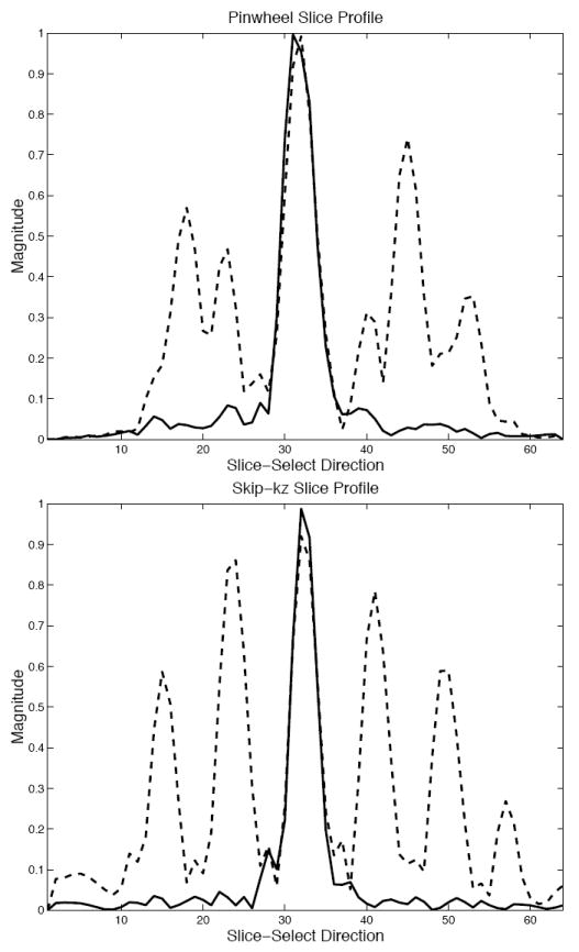
Plots of the magnitude profiles along the slice-select direction from the phantom images shown in Fig. 5 that were produced by excitation using four-shot pinwheel (top) and skip-k_z (bottom) 3D SSTRF pulses. The dashed and solid lines are the profiles produced from one shot and from all four shots, respectively.

Figure 7 shows brain images from the susceptibility artifact reduction experiments in humans. Figure 7 (a) and (b) show images of a typical 5 mm thick slice profile (x-z plane) acquired in the brain above the sinus from one and all four shots of the four-shot skip-k_z 3D SSTRF pulse. These images are qualitatively similar to both the simulations and the phantom images. The sidelobes present in Fig. 7 (a) are significantly reduced in (b). Figure 7 (c) and (d) show the same brain slice in using the four-shot skip-k_z 3D SSTRF pulse without and with a phase correction term. The small disk magnetization had a radius of approximately 1.5 cm and 5 points of shift (5π of phase dispersion through the slice). The image in Fig. 7 (d) shows recovery of signal magnitude in the sinus region compared to the image in shown in Fig. 7 (c). Figure 8 shows plots of the image magnitude profiles from the brain images indicated by the dotted lines in Fig. 7. The top plot shows profiles from Fig. 7 (a) and (b) along the slice select direction from the brain images excited with one (dashed line) and four (solid line) shots of the four-shot skip-k_z 3D SSTRF pulse. The magnitude of the residual signal from the sidelobes is 2-3% of the maximum signal of the central slice. The bottom figure shows a profile along the L-R direction from the brain slice shown in Fig. 7 (c) and (d) excited without (dashed line) and with (solid line) a localized linear through-plane phase correction in the 3D SSTRF pulse. There is approximately two times more signal in the sinus region using the pulse with the phase correction.

Figure 7.

Images (a) and (b) show 5 mm thick slice profiles (x-z plane) acquired in the brain above the sinus from one and all four shots of a four-shot skip-k_z 3D SSTRF pulse. The sidelobes in (a) are significantly reduced in (b). Images (c) and (d) show the same brain slice acquired using the four-shot skip-k_z 3D SSTRF pulse without and with a phase correction term. The image in (d) shows more signal magnitude in the sinus region than the image in (c). The dotted lines indicate the locations of the profile plots shown in Fig. 8.

Figure 8.

Plots of the magnitude profiles from the brain images shown in Fig. 7. The top figure shows a profile along the slice select direction excited with one (dashed line) and four (solid line) shots of the four-shot skip-k_z 3D SSTRF pulse used in Fig. 7. The magnitude of the residual signal from the sidelobes is 2-3% of the maximum signal. The bottom figure shows a profile along the L-R direction from the brain slice shown in Fig. 7 excited without (dashed line) and with (solid line) the localized linear through-plane phase correction in the 3D SSTRF pulse. There is approximately two times more signal magnitude in the sinus region using the pulse with the phase correction.

DISCUSSION

This work demonstrates that multi-shot 3D SSTRF pulses can be used to excite slices with arbitrary resolution through the use of simulations, phantom experiments, and human brain images. In all cases the simulated profiles agreed qualitatively with the actual profiles observed using the scanner for the flip angles used in the experiments. It was shown that at most four shots were needed to excite a 5 mm thick slice in the brain at 3T with reduced through-plane dephasing due to susceptibility induced field inhomogeneity. A four-shot pulse is practical for a number of fMRI experiments and is comparable to the number of steps needed for gradient compensation. An advantage of the multi-shot 3D SSTRF method is that theoretically an SNR increase equal to the square root of the number of shots is obtainable if flip angle is increased by a factor equal to the number of shots (28). Leaving the flip angle at the single-shot value will decrease SNR. Another advantage of the 3D SSTRF method over gradient compensation is that it is theoretically complete in its sampling requirements. Gradient compensation techniques tend to be arbitrary in the choice of step number and step size. As with gradient compensation, head motion is problematic. To investigate the effects of motion, we performed a simulation using a four shot skip-k_z 3D SSTRF pulse with parameters similar to those used in the brain imaging experiments. In the simulation, two of the shots were applied after a 1 cm in-plane displacement of the imaged object. We found that this introduced a variability of ±10%, more pronounced on the edges, in the excited magnetization profile. Variations of similar magnitude were introduced by a 1 cm through-plane shift. Although the utility of a multi-shot approach was stressed in this work, the 3D SSTRF is potentially a single-shot method. There are several approaches that can be used to reduce pulse length and shot number. Two possibilities are the use of variable density spiral trajectories and advanced imaging gradients. Variable density spiral methods are ideal for this technique because the magnetization profiles are already of the form of a Gaussian or other filter functions that do not require uniform sampling densities for the high spatial frequencies. Preliminary designs using variable density 3D SSTRF pulses show a 30% reduction in pulse length with little observable impact on the slice profiles. Further reductions in pulse length are possible with head gradient systems that are capable of high slew rates. A factor of four in slew rate will halve the length of the 3D SSTRF pulses.

Other works show multi-shot tailored RF methods can obtain high-resolution excitation profiles when used as inversion pulses. The use of tailored RF methods for slice-select pulses poses a greater demand on the sampling requirements needed for true slice selection. The slice-select nature of these pulses will also allow for multi-slice imaging applications. The ability to acquire multiple slices using the multi-shot 3D SSTRF method depends on the locations of the sidelobes produced by each individual shot for a given k-space trajectory. The maximum coverage along the slice-select direction using the skip-k_z design will be equal to the FOV along z divided by the number of shots. For the brain imaging example described above, this was 5 (20/4) cm or a maximum of ten 5 mm thick slices. The 90° rotations of the in-out spiral pairs, implemented to reduced the magnitude of the radial sidelobes, used in the pinwheel pulse design produced a z-dependence of the radial sidelobes. The rotations were actually unnecessary because the radial sidelobes appear outside of the imaged object. Removal of the 90° rotations but leaving in the in-out spirals will place the sidelobes at half of the FOV along z. This would allow for twenty 5 mm thick slices using a four-shot pulse with a 20 cm FOV along z. Another confound with multi-slice imaging is the need for extensive waveform memory. Each pulse had approximately 10,000 points (saved as short integers) for each of the five channels (rho, theta, x, y, and z) for each shot. This means that for a sixteen-slice, four-shot acquisition 131 (16 slices × 4 shots × 2 channels + 3 gradients) unique waveforms, or approximately 2.5 MB of free memory, are needed. Redundancy in the x, y, and z gradients has been exploited to reduce this number.

The shorter pulse lengths provided by the multi-shot 3D SSTRF pulse approach reduces the effects of both slice shifting due to field inhomogeneity and spatial variability of the echo time. The primary effect of off-resonance phase accrual during the pulse is a shift in the slice location along z (in-plane blurring effects can be ignored due to the relatively short length of the spirals in the pulse). Every n cycle of phase across the length of the pulse, produced by field inhomogeneity in a given spatial location, shifts that location an amount equal to n times the z-resolution of the pulse. For example, a 40 ms long 3D SSTRF pulse with a 1 mm resolution will experience a shift of 1 mm from a 0.15 radian/ms source of inhomogeneity, whereas a 160 ms pulse will experience a 4 mm shift. In particular, the accumulation of phase during the pulse needs to be accounted for in the design of the skip-k_z 3D SSTRF pulse, similar to multi-shot EPI (33). Each successive shot needs to be time-shifted an amount equal to the distance between z blips divided by the number of shots otherwise the cancellation of the sidelobes will be incomplete. The spatial variability of TE results from the feature that the RF pulse excites specific spatial locations at different times along the length of the pulse to correct for the localized through-plane intravoxel-dephasing artifact. The four-shot pulse used in this work, for example, excited the center of k-space of the region above the sinus approximately 2-3 ms earlier than the center of k-space of the rest of the brain to produce the through-plane phase correction in the frontal cortex. Therefore, the TE of the frontal cortex was approximately 2-3 ms longer than the TE of the rest of the brain. A comparable single-shot pulse would have an 8-12 ms variability. A 2-3 ms TE variability is not much of a concern in an application such as fMRI due to the wide range of TE’s over which adequate BOLD T2* contrast can be obtained.

One powerful feature of the 3D SSTRF method is that it allows for the use of anatomical maps of the desired magnitude and phase of the excited slice through the use of Eq. [3]. The analytical approximation given by Eq. [5] was used in this work because it greatly simplified the implementation of the technique. Furthermore, the measured phase maps will also allow for the correction of slice profile shifting due to the local field gradients and for spatially dependent TE effects. If we assume that the induced phase accumulation along the pulse is linear, Eq. [1] can be modified by including the multiplicative factor exp[iω(k(t))t], where ω(k)(t)) is the Fourier transform of the rate of phase change due to field inhomogeneity evaluated at each z blip. Spatial variability in the echo times in the slice due to the 3D SSTRF excitation can also be removed with the measured phase map because the shift in TE is directly proportional to the amount of through plane phase correction that is needed. Future work will focus on 3D SSTRF pulses that use in vivo maps of the desired phase distribution and the corrections for the above effects.

CONCLUSIONS

Three-dimensional slice-select tailored RF (3D SSTRF) pulse methods are useful for exciting arbitrary slice volumes. A major limitation of these methods is that unreasonably long pulse lengths are required for applications requiring high-resolution slice volumes. Problems associated with long pulses include off-resonance shifting, long echo times, and spatially varying TE’s. This work proposes the use of multi-shot 3D SSTRF pulses to overcome this limitation. Each shot of the 3D SSTRF pulse is applied in separate excitations and acquisitions. The final image is obtained by a complex summation of the images acquired from each individual excitation. The simulations and imaging experiments demonstrated that the two multi-shot approaches proposed, the pinwheel and skip-k_z stacked spiral trajectories, accurately excited slices with little contamination from sidelobes. The experiments using phantoms demonstrated that arbitrary patterns with high in-plane resolution can excited in the slice. Pulses were also designed that were capable of exciting a 5 mm thick slice with reduced through-plane dephasing artifacts in human brain images at 3T. The four-shot pulses used in this application were 40 ms long compared to the impractical 160 ms needed for a single-shot pulse with identical resolution.

References

- 1.Ahn CB, Kim JH, Cho ZH. High-speed spiral-scan echo planar NMR imaging- I. IEEE Transactions on Medical Imaging. 1986;MI-5:2–7. doi: 10.1109/TMI.1986.4307732. [DOI] [PubMed] [Google Scholar]
- 2.Meyer C, Hu B, Nishimura D, Macovski A. Fast Spiral Coronary Artery Imaging. Magn Reson Med. 1992;28:202–213. doi: 10.1002/mrm.1910280204. [DOI] [PubMed] [Google Scholar]
- 3.Noll DC, Cohen JD, Meyer CH, Schneider W. Spiral K-space MR Imaging of Cortical Activation. J Magn Reson Imaging. 1995;5:49–56. doi: 10.1002/jmri.1880050112. [DOI] [PubMed] [Google Scholar]
- 4.Mansfield P. Multi-planar image formation using NMR spin echoes. J Phys C. 1977;10:L55–L58. [Google Scholar]
- 5.Turner R, Bihan DL, Moonen C, Despres D, Frank J. Echo-planar time course MRI of cat brain oxygenation changes. Magn Reson Med. 1991;22:159–166. doi: 10.1002/mrm.1910220117. [DOI] [PubMed] [Google Scholar]
- 6.Belliveau J, Kennedy D, McKinstry R, Buchbinder B, Weisskoff R, Cohen M, Vevea J, Brady T, Rosen B. Functional mapping of the human visual cortex by magnetic resonance imaging. Science. 1991;254:716–719. doi: 10.1126/science.1948051. [DOI] [PubMed] [Google Scholar]
- 7.Ogawa S, Tank DW, Menon R, Ellerman JM, Kim S-G, Merkle H, Ugurbil K. Intrinsic signal changes accompanying sensory stimulation: Functional brain mapping with magnetic resonance imaging. Proc Natl Acad Sci USA. 1992;89:5951–5955. doi: 10.1073/pnas.89.13.5951. [DOI] [PMC free article] [PubMed] [Google Scholar]
- 8.Reese T, Davis T, Weisskoff R. Automated Shimming at 1.5T Using Echo-Planar Image Frequency Maps. J Magn Reson Imag. 1995;5(6):739–745. doi: 10.1002/jmri.1880050621. [DOI] [PubMed] [Google Scholar]
- 9.Noll DC, Meyer CH, Pauly JM, Nishimura DG, Macovski A. A homogeneity correction method for magnetic resonance imaging with time-varying gradients. IEEE Trans Med Imaging. 1991;10(4):629–637. doi: 10.1109/42.108599. [DOI] [PubMed] [Google Scholar]
- 10.Noll D, Pauly J, Meyer C, Nishimura D, Macovski A. Deblurring for Non-2D Fourier Transform Magnetic Resonance Imaging. Magnetic Resonance in Medicine. 1992;25(2):319–333. doi: 10.1002/mrm.1910250210. [DOI] [PubMed] [Google Scholar]
- 11.Irarrazabal P, Meyer CH, Nishmura DG, Macovski A. Inhomogeneity correction using an estimated linear field map. Magn Reson Med. 1996;35:278–282. doi: 10.1002/mrm.1910350221. [DOI] [PubMed] [Google Scholar]
- 12.Kadah YM, Hu X. Simulated phase evolution rewinding (SPHERE): A technique for reducing B0 inhomogeneity effects in MR images. Magn Reson Med. 1997;38:615–627. doi: 10.1002/mrm.1910380416. [DOI] [PubMed] [Google Scholar]
- 13.Constable R. Functional Imaging Using Gradient-Echo Echo-Planar Imaging in the Presence of Large Static Field Inhomogeneities. J Magn Reson Imag. 1995;5(6):746–752. doi: 10.1002/jmri.1880050622. [DOI] [PubMed] [Google Scholar]
- 14.Frahm J, Merboldt KD, Haenicke W. Direct FLASH MR Imaging of magnetic field inhomogeneities by gradient compensation. Magnetic Resonance in Medicine. 1988;6:474–480. doi: 10.1002/mrm.1910060412. [DOI] [PubMed] [Google Scholar]
- 15.Frahm J, Merboldt K-D, Hanicke W. The Influence of the Slice-Selection Gradient on Functional MRI of Human Brain Activation. J Magn Reson B. 1994;103:91–93. doi: 10.1006/jmrb.1994.1015. [DOI] [PubMed] [Google Scholar]
- 16.Yang Q, Edmister W, Kwong K, Demeure R, Smith M. Removal of Signal Loss Artifacts in T2*-Weighted EPI. Int Soc of Magn Reson in Med, 5th Scientific Meeting. 1998:1443. [Google Scholar]
- 17.Yang Q, Dardzinski B, Li S, Eslinger P, Smith M. Removal of Local Field Gradient Artifacts in T2*-Weighted Images at High Fields by Gradient-Echo Slice Excitation Profile Imaging. Magnetic Resonance in Medicine. 1998;39:402–409. doi: 10.1002/mrm.1910390310. [DOI] [PubMed] [Google Scholar]
- 18.Glover G. 3D z-Shim Method for Reduction of Susceptibility Effects in BOLD fMRI. Magnetic Resonance in Medicine. 1999;42:290–299. doi: 10.1002/(sici)1522-2594(199908)42:2<290::aid-mrm11>3.0.co;2-n. [DOI] [PubMed] [Google Scholar]
- 19.Haacke E, Tkach J, Parrish T. Reduction of T2* dephasing in gradient field-echo imaging. Radiology. 1989;170:457–462. doi: 10.1148/radiology.170.2.2911669. [DOI] [PubMed] [Google Scholar]
- 20.Zaim Y, Johnson G, Turnbull D. Sensitivity and Performance Time in MRI Dephasing Artifact Reduction Methods. Magnetic Resonance in Medicine. 2001;45:470–476. doi: 10.1002/1522-2594(200103)45:3<470::aid-mrm1062>3.0.co;2-e. [DOI] [PubMed] [Google Scholar]
- 21.Merboldt K-D, Finsterbusch J, Frahm J. Reducing Inhomogeneity Artifacts in Functional MRI of Human Brain Activation-Thin Slices vs Gradient Comepensation. Journal of Magnetic Resonance. 2000;145:184–191. doi: 10.1006/jmre.2000.2105. [DOI] [PubMed] [Google Scholar]
- 22.Cho Z, Ro Y. Reduction of susceptibility artifact in gradient-echo imaging. Magn Reson Med. 1992;23:193–200. doi: 10.1002/mrm.1910230120. [DOI] [PubMed] [Google Scholar]
- 23.Glover G, Lai S. Reduction of Susceptibility Effects in BOLD fMRI using Tailored RF Pulses. Int Soc of Magn Reson in Med, 6th Scientific Meeting. 1998:298. [Google Scholar]
- 24.Chen N, Wyrwicz A. Removal of Intravoxel Dephasing Artifact in Gradient-Echo Images Using a Field-Map Based RF Refocusing Technique. Magnetic Resonance in Medicine. 1999;42:807–812. doi: 10.1002/(sici)1522-2594(199910)42:4<807::aid-mrm25>3.0.co;2-8. [DOI] [PubMed] [Google Scholar]
- 25.Stenger VA, Boada FE, Noll DC. Three-Dimensional Tailored RF Pulses for the Reduction of Susceptibility Artifacts in T2*-Weighted Functional MRI. Magnetic Resonance in Medicine. 2000;44:525–531. doi: 10.1002/1522-2594(200010)44:4<525::aid-mrm5>3.0.co;2-l. [DOI] [PMC free article] [PubMed] [Google Scholar]
- 26.Pauly JM, Nishimura D, Macovski A. A k-space analysis of small-tip-angle excitation. J Magn Reson. 81:1989. 43–56. doi: 10.1016/j.jmr.2011.09.023. [DOI] [PubMed] [Google Scholar]
- 27.Hardy CJ, Bottomley PA. 31P Spectroscopic Localization using Pinwheel NMR Excitation Pulses. Magnetic Resonance in Medicine. 1991;17:315–327. doi: 10.1002/mrm.1910170204. [DOI] [PubMed] [Google Scholar]
- 28.Panych LP, Oshio K. Selection of High-Definition 2D Virtual Profiles with Multiple RF Excitations Along Interleaved Echo-Planar k-Space Trajectories. Magnetic Resonance in Medicine. 1999;41:224–229. doi: 10.1002/(sici)1522-2594(199902)41:2<224::aid-mrm2>3.0.co;2-g. [DOI] [PubMed] [Google Scholar]
- 29.Hardy CJ, Cline HE, Bottomley PA. Correcting for Nonuniform k-Space Sampling in Two-Dimensional NMR Selective Excitation. Journal of Magnetic Resonance. 1990;87:639–645. [Google Scholar]
- 30.Pauly JM, Hu BS, Wang SJ, Nishimura DG, Macovski A. A Three Dimensional Spin-Echo or Inversion Pulse. Magnetic Resonance in Medicine. 1993;29:2–6. doi: 10.1002/mrm.1910290103. [DOI] [PubMed] [Google Scholar]
- 31.Irarrazabal P, Nishimura D. Fast Three Dimensional Magnetic Resonance Imaging. Magn Reson Med. 1995;33(5):656–662. doi: 10.1002/mrm.1910330510. [DOI] [PubMed] [Google Scholar]
- 32.Glover GH. Simple Analytical Spiral K-Space Algorithm. Magnetic Resonance in Medicine. 1999;42:412–415. doi: 10.1002/(sici)1522-2594(199908)42:2<412::aid-mrm25>3.0.co;2-u. [DOI] [PubMed] [Google Scholar]
- 33.Feinberg D, Oshio K. Phase Errors in Multi-Shot Echo Planar Imaging. Magentic Resonance in Medicine. 1994;32:535–539. doi: 10.1002/mrm.1910320418. [DOI] [PubMed] [Google Scholar]