Biomedical Engineering Strategies in System Design Space

Abstract

Modern systems biology and synthetic bioengineering face two major challenges in relating properties of the genetic components of a natural or engineered system to its integrated behavior. The first is the fundamental unsolved problem of relating the digital representation of the genotype to the analog representation of the parameters for the molecular components. For example, knowing the DNA sequence does not allow one to determine the kinetic parameters of an enzyme. The second is the fundamental unsolved problem of relating the parameters of the components and the environment to the phenotype of the global system. For example, knowing the parameters does not tell one how many qualitatively distinct phenotypes are in the organism's repertoire or the relative fitness of the phenotypes in different environments. These also are challenges for biomedical engineers as they attempt to develop therapeutic strategies to treat pathology or to redirect normal cellular functions for biotechnological purposes. In this article, the second of these fundamental challenges will be addressed, and the notion of a “system design space” for relating the parameter space of components to the phenotype space of bioengineering systems will be focused upon. First, the concept of a system design space will be motivated by introducing one of its key components from an intuitive perspective. Second, a simple linear example will be used to illustrate a generic method for constructing the design space in which qualitatively distinct phenotypes can be identified and counted, their fitness analyzed and compared, and their tolerance to change measured. Third, two examples of nonlinear systems from different areas of biomedical engineering will be presented. Finally, after giving reference to a few other applications that have made use of the system design space approach to reveal important design principles, some concluding remarks concerning challenges and opportunities for further development will be made.

Introduction

One of the grand challenges in biology today is elucidation of the relationship between the information encoded in the genome and the context-dependent expression of that information as manifested in the phenotypic repertoire of an organism.² This also represents a major challenge for bioengineers in their attempt to model, predict and control biological processes with the aim of developing effective therapeutic strategies or optimizing a biotechnological process.

We now have a good idea of what is meant by the genotype, given the complete DNA sequence for the genome of numerous organisms including humans. However, it is not very clear regarding what is meant by the phenotype. At the level of the organism we have a sampling of phenotypes such as hair color of cats, shape and size of flowers, height and weight of livestock, not to mention disease states in humans. The difficulty in relating these two levels of biological organization and function is hard to over-estimate. Moreover, between the levels of genotype and phenotype of the organism there are many intervening levels that form a rich hierarchy of cell and molecular subsystems. Although there are some intuitive notions of what is meant by phenotype at the level of the organism, it is far from clear what the term phenotype means at the level of the intervening systems and what the phenotypic repertoire of any given system might be.

One approach to addressing these challenges involves the concept of a “system design space” in which qualitatively distinct phenotypes can be identified and counted, their relative fitness analyzed and compared, and their tolerance to global change measured.²⁵ In this context, consider the two fundamental challenges that need to be overcome in relating genotype to phenotype in a given environment: (1) the task of translating the genome sequence into the quantitative values for the parameters of the system, and (2) the task of translating a model of the system into the phenotype of the system in the given environment. The first task is the ongoing effort of experimental biology, and, whether considered from the bottom-up approach of molecular biology or the top-down approach of high-throughput technologies and computation, the magnitude of the problem is enormous.¹⁴ The difficulties of arriving at such a model involve issues of parameter estimation requiring model reduction⁷ and sensitivity analysis.¹² The second task, assuming that an explicit model or suite of models is in hand, is also a daunting problem. Exploring the full phenotypic potential of even a relatively small nonlinear model, say with 15 parameters, by analytic methods is intractable. Furthermore, simulations that involve an empirical sampling of alternative values suffer from a combinatorial explosion. (If one were to sample just 10 values of each parameter in all combinations it would require 10¹⁵ simulations, and one might still have missed some important behavior beyond the sampled range, or between the sampled points.)

This article addresses the second of these fundamental unsolved problems and shows how complex models consisting of nonlinear differential equations can be generically partitioned into a set of simpler sub-models expressed in a tractable canonical form. The conceptual framework is manifested graphically in a “system design space” consisting of well-defined regions in which specific constellations of parameters give rise to distinct behavior. In the general nonlinear case, the “form” of the equations characteristic of the sub-models differs from region to region, which provides the basis for defining “qualitatively distinct” phenotypes. For example, in one region the form of the equations might lead to behavior involving a square-root function, whereas in an adjacent region the form of the equations might lead to behavior involving a cubic function. In this manner the system design space relates the parameters of a model to its qualitatively distinct phenotypes. These concepts will be motivated first by considering the intuitive notion of a dominant sub-system model. Next, a simple pharmacokinetic model will be used to illustrate the steps in the generic construction of the system design space and the various types of comparative analysis that are facilitated by this approach. Two examples will then show areas of potential biomedical engineering application, one suggested by problems in targeted molecular imaging and the other by efforts to couple biochemical and biomechanical mechanisms in cell migration. Finally, a conclusion will give reference to other recent applications of the system design space methodology and summarize existing challenges and opportunities for further development.

Dominant Subsystems

A simple pharmacokinetic model illustrates one of the key features in the generic construction of the system design space for more complex models. When a drug is administered, here assumed to be by infusion, it becomes distributed with various concentrations among the organs of the body as a result of transport and biochemical reaction. Pharmacokinetic analysis utilizes compartmental models³ to predict this distribution as a function of parameters that characterize the drug and the various transport and reaction processes in the body.²⁰ A simplified case involving two compartments is represented in Fig. 1, with compartment 1 being nonspecific and compartment 2 being the specific target for the drug.

FIGURE 1.

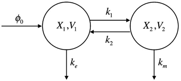
Two-compartment pharmacokinetic model. A drug is infused into the blood stream at a constant rate ϕ₀. The drug has concentration X₁ in compartment 1, which represents the blood with volume V₁, is excreted by a first-order process with rate constant k_e, and is transported to compartment 2 with a rate constant k₁. The drug has concentration X₂ in compartment 2, which represents the target organ with volume V₂, is metabolized by a first-order process with rate constant k_m, and is transported to compartment 1 with a rate constant k₂. The relative sizes of the compartments is given by ρ = V₂/V₁.

What is the repertoire of qualitatively distinct phenotypes for this simple system? If we could analytically solve for the steady states of this system, then we might be able to characterize the fixed points and the local dynamics they represent as well as identify distinct operating regimes from the structure of the solution.

Phenotypes from the Analytic Solution

In fact, we can solve for the steady-state behavior of this simple linear system. The differential equations governing this system,

$$\begin{array}{l}\frac{d{X}_1}{\mathit{\text{dt}}}={\phi }_0+\rho k_2{X}_2-k_1{X}_1-k_{\text{e}}{X}_1\hfill \\ \rho \frac{d{X}_2}{\mathit{\text{dt}}}=k_1{X}_1-\rho k_2{X}_2-\rho k_{\text{m}}{X}_2\hfill \end{array}$$ (1)

yield the following steady-state solution:

$$\begin{array}{l}{X}_1=\frac{{\phi }_0{k}_2+{\phi }_0{k}_{\text{m}}}{k_{\text{1}}{k}_{\text{m}}+k_{\text{e}}{k}_2+k_{\text{e}}{k}_{\text{m}}}\hfill \\ X_2=\frac{{\phi }_0{k}_1/\rho }{k_{\text{1}}{k}_{\text{m}}+k_{\text{e}}{k}_2+k_{\text{e}}{k}_{\text{m}}}.\hfill \end{array}$$ (2)

The solution is characterized by the relative volumes of the compartments (ρ = V₂/V₁) that can be considered as fixed, two kinetic parameters representing transport (k₁ and k₂) and two kinetic parameters representing excretion and metabolism of the drug (k_e and k_m) that might be subject to change with the design of a drug, and an infusion rate (ϕ₀) that is subject to direct experimental manipulation.

The solution in Eq. (2) suggests six qualitatively distinct phenotypes based on the dominance of terms in the numerator and denominator of each expression. By dominance, we mean that, in each component of the solution, there is one term in the numerator that is larger in value than the other terms while there is one term in the denominator that is larger than the others; there is no dominance if there are terms that contribute equally to the numerator or denominator. However, two of the six in this case are invalid because the conditions for dominance cannot be satisfied (if the first term in the numerator of X₁ is dominant over the second, then it is impossible for the third term to be dominant over the second in the denominator; conversely, if the second term in the numerator of X₁ is dominant over the first, then it is impossible for the second term to be dominant over the third in the denominator). Thus, four qualitatively distinct phenotypes can be identified for this system.

$$\begin{array}{l}\text{Case}1:X_1\approx \frac{{\phi }_0}{k_1}\text{and}{X}_2\approx \frac{{\phi }_0}{\rho k_{\text{m}}},\\ \text{for}{k}_{\text{m}}>k_2\text{and}{k}_{\text{e}}<k_1\end{array}$$ (3)

$$\begin{array}{l}\text{Case}2:X_1\approx \frac{{\phi }_0}{k_{\text{e}}}\text{and}{X}_2\approx \frac{{\phi }_0{k}_1}{\rho k_{\text{e}}{k}_{\text{m}}},\\ \text{for}{k}_{\text{m}}>k_2\text{and}{k}_{\text{e}}>k_1\end{array}$$ (4)

$$\begin{array}{l}\text{Case}3:X_1\approx \frac{{\phi }_0{k}_2}{k_1{k}_{\text{m}}}\text{and}{X}_2\approx \frac{{\phi }_0}{\rho k_{\text{m}}},\\ \text{for}{k}_{\text{m}}<k_2\text{and}{k}_{\text{e}}{k}_2<k_1{k}_{\text{m}}\end{array}$$ (5)

$$\begin{array}{l}\text{Case}4:X_1\approx \frac{{\phi }_0}{k_{\text{e}}}\text{and}{X}_2\approx \frac{{\phi }_0{k}_1}{\rho k_{\text{e}}{k}_{\text{2}}},\\ \text{for}{k}_{\text{m}}<k_2\text{and}{k}_{\text{e}}{k}_2>k_1{k}_{\text{m}}.\end{array}$$ (6)

An example to illustrate the physical meaning of dominance in this case is the following. The concentration of drug in the specific compartment (X₂) is the same for Cases 1 and 3 (determined by the volumes of the compartments and metabolism of the drug in compartment 2); whereas that in the non-specific compartment (X₁) is less for Case 1 (determined by the transport from compartment 1) than that for Case 2 (which is also determined by the transport from compartment 2 being greater than the metabolism in compartment 2).

This provides an attractive approach to the identification of molecular phenotypes when an analytic solution is available. However, such a solution is seldom available for the more complex nonlinear systems that are characteristic of nearly all biomedical engineering systems of interest.

Phenotypes from the Differential Equation

Might the same approach, based on the identification of dominant terms, be applied to the differential equation without having an analytic solution? The answer is yes, as shown below.

Examination of Eq. (1) suggests potentially eight qualitatively distinct phenotypes based on dominance among the positive and negative terms. However, four of these are invalid because the conditions for dominance cannot be satisfied. The remaining four cases are the following:

$$\begin{array}{l}\text{Case}1:\frac{d{X}_1}{dt}\approx {\phi }_0-k_1{X}_1\text{and}\rho \frac{d{X}_2}{dt}\approx k_1{X}_1-\rho k_{\text{m}}{X}_2\\ \text{for}{k}_{\text{m}}>k_2\text{and}{k}_{\text{e}}<k_1\end{array}$$ (7)

$$\begin{array}{l}\text{Case}2:\frac{d{X}_1}{dt}\approx {\phi }_0-k_{\text{e}}{X}_1\text{and}\rho \frac{d{X}_2}{dt}\approx k_1{X}_1-\rho k_{\text{m}}{X}_2\\ \text{for}{k}_{\text{m}}>k_2\text{and}{k}_{\text{e}}>k_1\end{array}$$ (8)

$$\begin{array}{l}\text{Case}3:\frac{d{X}_1}{dt}\approx \rho k_2{X}_2-k_1{X}_1\text{and}\rho \frac{d{X}_2}{dt}\approx k_1{X}_1-\rho k_2{X}_2\\ \text{for}{k}_{\text{m}}<k_2,k_{\text{e}}<k_1\text{and}{k}_{\text{e}}{k}_2<k_1{k}_{\text{m}}\end{array}$$ (9)

$$\begin{array}{l}\text{Case}4:\frac{d{X}_1}{dt}\approx {\phi }_0-k_{\text{e}}{X}_1\text{and}\rho \frac{d{X}_2}{dt}\approx k_1{X}_1-\rho k_2{X}_2\\ \text{for}{k}_{\text{m}}<k_2\text{and}{k}_{\text{e}}>k_1.\end{array}$$ (10)

Case 3 is rank deficient and requires a different treatment as discussed in the following paragraph. Thus, four qualitatively distinct phenotypes can be identified for this system. This method of selecting one dominant positive term and one dominant negative term generates a local S-system,^21,22 which for more complex systems is a specific class of ordinary nonlinear differential equations within the power-law formalism, that in steady state reduces to a linear system for which there is an explicit steady-state solution. The steady-state solutions of Eqs. (7), (8), and (10) are obtained by setting the derivatives to zero and solving for the dependent variables, and the results are seen to be exactly the same as those in Eqs. (3), (4), and (6).

Case 3 exhibits a singularity that is removed when placed in the context of the full system, and it is actually composed of two sub-cases. This situation arises because there is a dominant rapid equilibrium between X₁ and X₂, which causes the other terms, representing fluxes into or out of these pools, to be neglected. This leads to a linear dependency in the solution that dictates a constraint between X₁ and X₂. In effect, the rapid equilibrium causes these pools to behave as an aggregate of the two pools in the context of the complete model, thereby creating a virtual branch point with a single influx (ϕ₀) and two effluxes (loss from either the X₁ or the X₂ pool). The selection of a dominant loss term from the virtual branch point yields an additional dominance condition. The constraint relation between X₁ and X₂, together with the steady-state equation that results from the choice of a dominant loss term, yields the steady-state solution. For this solution to be valid, it must satisfy all of the dominance conditions (the original ones plus the additional one associated with the virtual branch point).

The first sub-case of Eq. (9) is

$$\begin{array}{l}\text{Case}3:\frac{d{X}_1}{dt}\approx \rho k_2{X}_2-k_1{X}_1\text{and}\rho \frac{d{X}_2}{dt}={\phi }_0-\rho k_{\text{m}}{X}_2\\ \text{for}{k}_{\text{m}}<k_2\text{and}{k}_{\text{e}}{k}_2<k_1{k}_{\text{m}}\end{array}$$

which has a steady-state solution that is identical to that of Case 3 determined from the analytic solution [Eq. (5)]. The second sub-case, is the following:

$$\begin{array}{l}\text{Case}3\prime :\frac{d{X}_1}{dt}\approx {\phi }_0-k_{\text{e}}{X}_1\text{and}\rho \frac{d{X}_2}{dt}=k_1{X}_1-\rho k_2{X}_2\\ \text{for}{k}_{\text{e}}<k_1\text{and}{k}_{\text{e}}{k}_2>k_1{k}_{\text{m}}\end{array}$$

which has a steady-state solution that is identical to that of Case 4 [Eq. (6)]; thus, it also can be considered as a sub-case Case 4′.

Thus, after this situation with sub-cases is taken into account, both methods—the one based on the analytic solution and the other based on the differential equations—generate exactly the same set of four cases. The method involving dominance among positive and negative terms in the differential equation has several advantages. First, solving for the steady state of Eqs. (7)–(10) is much simpler than solving for the full analytic solution. Moreover, as we shall see shortly, the steady-state solution of the differential equations resulting from dominant terms can be obtained for more general cases, including systems that have no corresponding analytic solution. Second, having the differential equations based on dominant positive and negative terms means that we also have access to the local dynamic behavior for each of the cases.^21,22 However, can this method tell us how many distinct phenotypes the system is capable of exhibiting? By integrating all the information from the steady-state solutions and their corresponding boundaries, we can address this question in the context of the system design space.^9,25

Phenotypes in System Design Space

The conditions that must be met to justify dominance among the positive and negative terms can be expressed in terms of the ratios k_m/k₂ and k_e/k₁, and summarized as follows:

$$\begin{array}{l}\text{Case}1:\frac{k_{\text{m}}}{k_2}>1\text{and}\frac{k_{\text{e}}}{k_1}<1\\ \text{Case}2:\frac{k_{\text{m}}}{k_2}>1\text{and}\frac{k_{\text{e}}}{k_1}>1\\ \text{Case}3:\frac{k_{\text{m}}}{k_2}>\frac{k_{\text{e}}}{k_1}\text{and}\frac{k_{\text{m}}}{k_2}<1\\ \text{Case}4:\frac{k_{\text{m}}}{k_2}<\frac{k_{\text{e}}}{k_1}\text{and}\frac{k_{\text{e}}}{k_1}<1.\end{array}$$

The result is a set of boundaries delimiting regions that define qualitatively distinct phenotypes of the system. These regions can be visualized graphically in the system design space as shown in Fig. 2.

FIGURE 2.

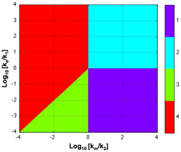
System design space for the model in Fig. 1. Case 1 (Purple): the same dominant flux into pool 1, between pool 1 and pool 2, and from pool 2 by metabolism. Case 2 (Blue): a dominant flux into pool 1 and from pool 1 by excretion; a second dominant flux into pool 2 and from pool 2 by metabolism. Case 3 (Green): rapid quasi-equilibrium between pools 1 and 2; an influx to pool 1 and an equivalent efflux from pool 2. Case 4 (Red): rapid quasi-equilibrium between pools 1 and 2; an influx to pool 1 and an equivalent efflux from pool 1 by excretion. See Fig. 3 and text for discussion.

Enumeration of Phenotypes

The primary function of the system design space is to precisely define boundaries between regions of qualitatively distinct phenotypes. In retrospect, these phenotypes can be seen to agree with our intuition for this simple system; there are four distinct phenotypes as depicted in Fig. 3. Case 1: There is an essentially irreversible flux through pool 1 into pool 2 and out of pool 2 (lower right-hand quadrant). Case 2: There is an irreversible flux into and out of pool 1 and a smaller essentially irreversible flux into and out of pool 2 (upper right-hand quadrant). Case 3: There is a small irreversible flux into pool 1 matched by an irreversible flux out of pool 2 and a rapid quasi-equilibrium flux between pools 1 and 2 (lower portion of the lower left-hand quadrant). Case 4: There is an irreversible flux into and out of pool 1 and a small equilibrium flux between pools 1 and 2 (upper left-hand quadrant), or a small irreversible flux into and out of pool 1 and a large rapid equilibrium flux between pools 1 and 2 (upper portion of the lower left-hand quadrant).

FIGURE 3.

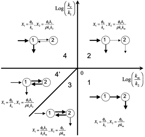
System design space for the model in Fig. 1. In each phenotypic region the pools associated with the variables X₁ and X₂ are represented graphically. The relative thickness of the arrows suggests the dominant fluxes for each pool. See legend for Fig. 2 and text for discussion.

Accuracy

Clearly the approximate solutions and the actual solution will only agree quantitatively in regions far removed from the boundaries; by definition, there is no dominance at the boundaries. A plot of the system design space with the z-axis representing the differences between the actual values of X₁ and X₂ and their approximate values in each region (Fig. 4) shows that the maximum error occurs along the boundaries (the vertical and horizontal axis and the diagonal line). Discrepancies will occur in the neighborhood of the boundaries, which are intended to identify changes in qualitative phenotype, and so care needs to be exercised in evaluating the situation near the boundaries.

FIGURE 4.

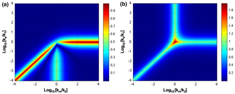
Accuracy of representation within system design space for the model in Fig. 1. (a) X₁ and (b) X₂. Differences between the values determined by the analytic solution and by the approximate solution within each phenotypic region are shown as a heat map on the z-axis. Error is measured as fold difference relative to the actual value. See text for discussion.

Dynamics

Another pharmacokinetic application, perhaps the more common, involves the periodic administration of a drug as a bolus rather than as a constant infusion. In this case, the input to the X₁ pool is a bolus, assumed to mix rapidly, that raises the concentration instantaneously from X_1,Min to X_1,Max, and there is loss from the pool for a period Δt until the next bolus is administered (Fig. 5).

FIGURE 5.

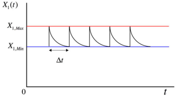
Concentration in pool 1 for the model in Fig. 1 when the input ϕ₀(t) is a periodic bolus. See text for discussion.

The differential equations that govern the system from one bolus to the next, t_i < t < t_i + Δt, for Case 1 (k₁ > k_e and k_m > k₂) are the following:

$$\frac{d{X}_1}{dt}\approx -k_1{X}_1\text{and}\rho \frac{d{X}_2}{dt}\approx k_1{X}_1-\rho k_{\text{m}}{X}_2.$$

The solution for X₁(t) is a simple decaying exponential function whose final value before the next bolus is given by

$$X_{1,\text{Min}}=X_{1,\text{Max}}exp(-k_1\Delta t).$$

The average value of X₁(t) is given by

$$\langle X_1(t)\rangle =\frac{{\int }_{t_i}^{t_i+\Delta t}{X}_{1,max}{e}^{-k_{1}t}dt}{\Delta t}=\frac{X_{1,\text{max}}}{k_1\Delta t}\left[1-e^{-k_1\Delta t}\right].$$

If the bolus is defined as ΔX₁ = X_1,Max − X_1,Min, then

$$\langle X_1(t)\rangle =\frac{X_{1,\text{max}}}{k_1\Delta t}\left[1-e^{-k_1\Delta t}\right]=\frac{1}{k_1\Delta t}\Delta X_1.$$ (11)

The corresponding average value for X₂(t) is given by

$$\langle X_2(t)\rangle =\frac{k_1}{\rho k_{\text{m}}}\langle X_1(t)\rangle .$$ (12)

The averages for the other cases are obtained in a similar fashion. Thus,

$$\text{Case}2:\langle X_1(t)\rangle =\frac{1}{k_{\text{e}}\Delta t}\Delta X_1\text{and}\langle X_2(t)\rangle =\frac{k_1}{\rho k_{\text{m}}}\langle X_1(t)\rangle$$ (13)

$$\text{Case}3:\langle X_1(t)\rangle =\frac{1}{k_{\text{m}}\Delta t}\Delta X_1\text{and}\langle X_2(t)\rangle =\frac{k_1}{\rho k_2}\langle X_1(t)\rangle$$ (14)

$$\text{Case}4:\langle X_1(t)\rangle =\frac{1}{k_{\text{e}}\Delta t}\Delta X_1\text{and}\langle X_2(t)\rangle =\frac{k_1}{\rho k_{\text{2}}}\langle X_1(t)\rangle .$$ (15)

It should be noted that ΔX₁ is not the actual bolus in Case 3, instead it is less by the fraction ρk₂/(k₁ + ρk₂) because of the rapid equilibrium between the two pools.

If the parameters and the constant infusion rate locate the operating point in a particular phenotypic region of the system design space, then the same operating point would be established on average with frequent small boluses. From the Eqs. (11)–(15), one can see that there is a tradeoff between the dominant rate constants and the period between boluses. In Case 4, if k_e can be made small then Δt can be large and the concentration of X₁(t) will be maintained with small fluctuations about its average. For example, suppose the aim is to maintain an average concentration of X₁ = 95 units and stay between a maximum concentration of 100 and a minimum of 90. This could be achieved with a dose of 10 units every 12 h provided the first-order rate constant for excretion of the drug k_e is approximately 0.211 per day, or every 4 h if k_e is ∼0.632 per day.

This is consistent with existing strategies in which one aims to design a drug that has the preferred distribution (pool X₂ vs. X₁) and slow decay, generally k_e ≪ k₁ and k_m ≪ k₂, thereby allowing for long periods between doses.

Evaluating Phenotypes

The performance of the system represented within each of the phenotypic regions can be assessed and compared according to both local and global criteria.

Local Performance

The local performance in each of the phenotypic regions can be readily compared on the basis of relevant quantitative criteria, since the system representation within each phenotypic region is in general a simple but nonlinear S-system within the power-law formalism for which determination of local behavior reduces to conventional linear analysis.^22,21 Thus, the behavior involving local (small) variations is completely determined and there are criteria that can be defined and evaluated to characterize performance of the system. These criteria are quantified using logarithmic gains, parameter sensitivities, and response times.

Logarithmic gains in concentrations and fluxes in response to changes in value for an independent variable are defined by the relative derivative of the explicit steady-state solution. For example, using the concentration X₁, metabolic flux ϕ_m and independent infusion rate ϕ₀, representative logarithmic gains for the system in Fig. 1 are:

$$\begin{array}{l}L(X_1,{\phi }_0)=\frac{\partial \text{Log}{X}_1}{\partial \text{Log}{\phi }_0}=\frac{\partial X_1}{\partial {\phi }_0}\frac{{\phi }_0}{X_1},\\ L({\phi }_m,{\phi }_0)=\frac{\partial \text{Log}{\phi }_m}{\partial \text{Log}{\phi }_0}=\frac{\partial {\phi }_m}{\partial {\phi }_0}\frac{{\phi }_0}{{\phi }_m}.\end{array}$$

Parameter sensitivities of such state variables in response to changes in value for the parameters that define the structure of the system (e.g., the independent rate constants) are defined by the relative derivative of the explicit steady-state solution. For example,

$$\begin{array}{l}S(X_1,k_{-1})=\frac{\partial \text{Log}{X}_1}{\partial \text{Log}{k}_{-1}}=\frac{\partial X_1}{\partial k_{-1}}\frac{k_{-1}}{X_1},\\ S({\phi }_{\text{e}},k_2)=\frac{\partial \text{Log}{\phi }_{\text{e}}}{\partial \text{Log}{k}_2}=\frac{\partial {\phi }_{\text{e}}}{\partial k_2}\frac{k_2}{{\phi }_{\text{e}}}.\end{array}$$

Response times are determined by the inverse of the real part of the dominant eigenvalue.

Comparisons of Local Performance

The local performance of designs in the various phenotypic regions can be readily compared on the basis of relevant quantitative criteria. For this didactic example, let us postulate the four criteria in Table 1. Criteria 1–3 are relevant for maximizing the steady-state fraction of drug in the specific compartment (compartment 2 in Fig. 1); Criterion 4 is relevant for persistence of the drug in the specific compartment following a bolus of input. The comparative results are summarized in Table 2.

TABLE 1. Criteria for the local performance of the system in Fig. 1.

Criterion number	Definition	Calculation
1	Maximize the gain in concentration X2 in response to changes in input flux ϕ0	Max L (X2, ϕ0)
2	Maximize ratio of X2 to X1	Max (X2/X1)
3	Maximize robustness of concentration X2 to variations in parameters pi	Min Σi|S(X2, pi)|
4	Maximize response time	Max τ1/2 (Max λ)

TABLE 2. Comparison of local performance in the four phenotypic regions of Fig. 2.

	Criteriona
Phenotypic region	1 ⇑b	2 ⇑	3 ⇓	4 ⇓
1	1	k1/(ρkm)	2	1/k2
2	1	k1/(ρkm)	4	1/ke
3	1	k1/(ρk2)	4	1/ke
4	1	k1/(ρk2)	2	1/km

^aThe criteria are described in the text and their quantification is defined in Table 1.

^bTo improve the performance according to the definitions in Table 1, one must have either a high (⇑) or a low (⇓) value for the associated criterion.

All the phenotypic regions are equivalent with respect to the logarithmic gain in the concentration of the target pool, X₂, with respect to a change in the input, ϕ₀ (Criterion 1). Phenotypic regions 1 and 4 are best with respect to robustness (Criterion 3). There is a tradeoff between phenotypic regions 1 and 4 with respect to the ratio of the target pool, X₂, to the nonspecific pool, X₁ (Criterion 2) and response time (Criterion 4): when region 1 is better than region 4 with respect to Criterion 2, region 4 is better than region 1 with respect to Criterion 4, and vice a versa. Thus, phenotypic regions 1 and 4 exhibit the best performance, with a tradeoff between Criteria 2 and 4. This implies the following relationship among the parameters: 1 > k_m/k₂ > k_e/k₁ when the tradeoff favors Case 4, and k_m/k₂ > 1 > k_e/k₁ when it favors Case 1.

Global Tolerance

Large changes in parameters and independent variables can change the qualitative character of the phenotype, in some cases from one that is physiological to one that is pathological. In order to characterize such large changes we need a global equivalent of local robustness, which is defined as insensitivity to local changes. We call this concept global tolerance and define it as the value of a parameter at the boundary between adjacent phenotypic regions relative to the normal operating value within a region, or the inverse if the normal value is greater than the value at the boundary.⁵ We will use the expression “[T_D, T_I]” to describe the global tolerances, where T_D = tolerance to a fold decrease and T_I = tolerance to a fold increase (since boundaries can be crossed either by decreasing or increasing the value of a parameter).

For purposes of illustration, let us assume operating points in each of the four regions depicted in Fig. 2. In phenotypic region 1 we shall assume the nominal values are Log(k_m/k₂) = +2 and Log(k_e/k₁) = −1. Although the global tolerances for each of the parameters and independent variables will require a calculation in general, the geometry of the system design space in Fig. 2 is so simple that one can determine the global tolerances from the boundaries by inspection. In this case, the results are shown on the first line of entries in Table 3; similar results are shown on subsequent lines for the other regions and assumed operating points. These results make evident a number of symmetries in this system. Since the assumed operating points were all well removed from the boundaries, it is not surprising that the tolerances are all large fold changes, which is in contrast to the values for local robustness, which are often manifested as percentage changes.

TABLE 3. Global tolerances to change in parameters and independent variables with assumed values for each of the operating points in the system design space (see Fig. 2).

		Parameters
Region	Log (operating point)	ke	k1	km	k2
1	(+2, −2)	[100, ∞]a	[∞, 100]	[100, ∞]	[∞, 100]
2	(+2, +1)	[∞, 10]	[10, ∞]	[100, ∞]	[∞, 100]
3	(−2, +1)	[∞, 10]	[10, ∞]	[∞, 100]	[100, ∞]
4	(−1, −2)	[100, ∞]	[∞, 100]	[10, 10]	[10, 10]

^aNotation: [fold decrease, fold increase].

The criteria for effective performance will vary depending upon the system of interest, but the types of calculations needed to characterize the local and global behavior typically will be the same. However, the details of the calculations will become more complex for realistic systems. Examples can be found in the following sections and in the references cited in the “Conclusion” section. Although the entire analysis and plotting in this case could be accomplished analytically, for more complex systems this becomes impractical. A Matlab Toolbox has been developed to assist in the construction and analysis of the system design space.⁹ Its use will be illustrated in the following examples of more realistic applications.

Targeted Molecular Imaging

In the search for agents that can be specifically targeted to tumors for their localization and destruction, extensive in vitro testing is used to identify lead compounds. However, in vitro success does not always correspond to in vivo success for reasons that are not always understood; as a result, many compounds with favorable in vivo characteristics may be overlooked. Gagnon et al.¹⁰ have addressed this issue by developing a method for high-throughput in vivo screening of targeted molecular imaging agents based on the one-bead-one-compound (OBOC) library approach,^11,15 fast and efficient solid-phase radiolabeling,^13,26 and in vivo imaging with microPET.^18,27 This approach allows promising compounds that might have escaped detection during in vitro screening to be identified much earlier in the development process (i.e., providing a go or no-go decision to be made sooner). An example of the imaging results for a mouse with two tumors, one targeted (termed the positive tumor in the original studies) and the other non-targeted (termed the negative tumor) by the specific test peptide is shown in Fig. 6. In some cases, counterintuitive results are obtained when compounds with high affinity give poorer results than compounds with lower affinity.¹⁰

FIGURE 6.

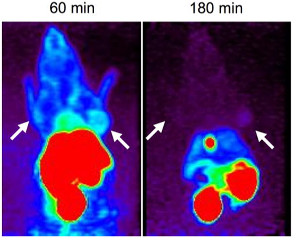
MicroPET images obtained from one of the most promising lead peptides obtained from high-throughput screening. Arrows indicate location of positive and negative tumors at 60 and 180 min following injection of the test peptide. The animal is oriented supine and the α_vβ₆-positive tumor is on the right side of the mouse. From Gagnon et al.¹⁰

The effectiveness of targeting can be analyzed using compartmental models. Although a fully developed realistic model will not be attempted here, a simplified model (Fig. 7) that illustrates features of the system design space approach, without performing a full analysis, will begin to address the method developed by Gagnon et al.¹⁰

FIGURE 7.

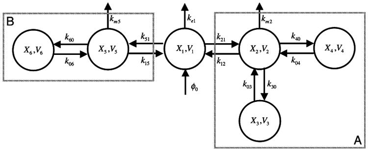
Six-compartment model. Compartment 1 represents the blood with volume V₁ and free peptide concentration X₁. Compartment A represents the tissue type in which the tumors are transplanted. Compartment 2 represents the non-tumor tissue with volume V₂ and free peptide concentration X₂. Compartment 3 represents the positive-tumor with volume V₃ and bound-peptide with concentration X₃. Compartment 4 represents the negative-tumor with volume V₄ and bound-peptide concentration X₄. Compartment B represents an aggregate of all other tissues in the body. Compartment 5 represents this aggregate with volume V₅ and free peptide concentration X₅. Compartment 6 represents non-specific targets within this aggregate with volume V₆ and bound-peptide concentration X₆ (see text for discussion).

Phenotypes from the Differential Equations

The set of differential equations governing the system represented in Fig. 7 is

$$\begin{array}{cc}\hfill \frac{d{X}_1}{dt}& ={\phi }_0+k_{12}{\rho }_{21}{X}_2+k_{15}{\rho }_{51}{X}_5-k_{\text{e}1}{X}_1-k_{21}{X}_1-k_{51}{X}_1\hfill \\ \hfill {\rho }_{21}\frac{d{X}_2}{dt}& =k_{21}{X}_1+k_{03}{\rho }_{31}{X}_3+k_{04}{\rho }_{41}{X}_4-k_{\text{m}2}{\rho }_{21}{X}_2-k_{12}{\rho }_{21}{X}_2-k_{30}{\rho }_{31}{V}_2{X}_2{T}_{3\text{f}}-k_{40}{\rho }_{41}{V}_2{X}_2{T}_{4\text{f}}\hfill \\ \hfill \frac{d{X}_3}{dt}& =k_{30}{V}_2{X}_2{T}_{3\text{f}}-k_{03}{X}_3\hfill \\ \hfill \frac{d{X}_4}{dt}& =k_{40}{V}_2{X}_2{T}_{4\text{f}}-k_{04}{X}_4\hfill \\ \hfill {\rho }_{51}\frac{d{X}_5}{dt}& =k_{51}{X}_1+k_{06}{\rho }_{61}{X}_6-k_{\text{m}5}{\rho }_{51}{X}_5-k_{15}{\rho }_{51}{X}_5-k_{60}{\rho }_{61}{V}_5{X}_5{T}_{6\text{f}}\hfill \\ \hfill \frac{d{X}_6}{dt}& =k_{60}{V}_5{X}_5{T}_{6\text{f}}-k_{06}{X}_6\hfill \end{array}$$ (16)

where the relative volumes ρ_ij = V_i/V_j, single-site binding is assumed for each target, and the concentration of total target for each type T_i is conserved (i.e., the concentration of free target T_if = the concentration of total target T_i − the concentration of bound target X_i). The corresponding set of steady-state equations is the following:

$$\begin{array}{c}0={\phi }_0+k_{12}{\rho }_{21}{X}_2+k_{15}{\rho }_{51}{X}_5-k_{\text{e}1}{X}_1-k_{21}{X}_1-k_{51}{X}_1\hfill \\ 0=k_{21}{X}_1-k_{\text{m}2}{\rho }_{21}{X}_2-k_{12}{\rho }_{21}{X}_2\hfill \\ 0=k_{30}{V}_2{X}_2{T}_{3\text{f}}-k_{03}{X}_3\hfill \\ 0=k_{40}{V}_2{X}_2{T}_{4\text{f}}-k_{04}{X}_4\hfill \\ 0=k_{51}{X}_1-k_{\text{m}5}{\rho }_{51}{X}_5-k_{15}{\rho }_{51}{X}_5\hfill \\ 0=k_{60}{V}_5{X}_5{T}_{6\text{f}}-k_{06}{X}_6\hfill \\ 0=T_3-X_3-T_{3\text{f}}\hfill \\ 0=T_4-X_4-T_{4\text{f}}\hfill \\ 0=T_6-X_6-T_{6\text{f}}.\hfill \end{array}$$ (17)

A bound on the total number T of qualitatively distinct phenotypic regions is given by the number of combinations involving the number of positive P_i and negative N_i terms in the n equations:

$$T=\prod _{i=1}^n(P_i\ast N_i).$$

In this case, T = (3 * 3)(1 * 2)(1 * 1)(1 * 1)(1 * 2) (1 * 1)(1 * 2)(1 * 2)(1 * 2) = 288. Assuming nominal values for the parameters based on data from Gagnon et al.¹⁰ yields the system design space in Fig. 8 with only four valid regions. Moreover, in steady state

FIGURE 8.

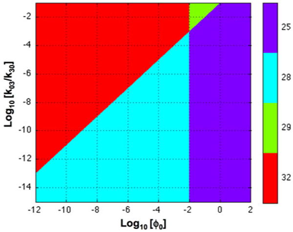
System design space for the system in Fig. 7. The x-axis represents the various levels of peptide input, ϕ_o, and the y-axis represents the equilibrium dissociation constant for binding to the positive tumor, k₀₃/k₃₀. The nominal values of the parameters in arbitrary units are assumed to be the following: k₁₂ = k₂₁ = k₁₅ = k₅₁ = 1300, V₁ = 10⁴, V₂ = 10³, V₃ = V₄ = 10, V₅ = 10⁴, V₆ = 10³, T₃ = 10, T₄ = T₆ = 1.5 × 10⁶, k₃₀ = k₄₀ = k₆₀ = 1, k₀₃ = 10⁻⁸, k₀₄ = k₀₆ = 10⁻³, k_m2 = k_m5 = 10⁻⁹, k_e1 = 10⁵, and ϕ₀ = 10⁻⁵. The numbering of the regions and the corresponding color are indicated in the sidebar. The plot was generated by using the Design Space Toolbox.⁹

$$\begin{array}{cc}\hfill V_5{X}_5& =\frac{k_{51}(k_{\text{m}2}+k_{12})}{k_{21}(k_{\text{m}5}+k_{15})}{V}_2{X}_2\hfill \\ \hfill X_3& =\frac{T_3{V}_2{X}_2}{(K_3+V_2{X}_2)},X_4=\frac{T_4{V}_2{X}_2}{(K_4+V_2{X}_2)},X_6=\frac{T_6{V}_5{X}_5}{(K_6+V_5{X}_5)}\hfill \end{array}$$

where the equilibrium dissociation constant for the bound targets is K_i = k_0i/k_i0.

Discrimination Ratios

We assume that the positive tumor has the same non-specific targets as the negative tumor, and that the total amount of bound target is the product of the concentration of bound target and a corresponding volume. If we make the further simplifying assumption that the initial peak values are represented by a large value of ϕ₀ (in region 25), and that a quasi-steady state is established, which slowly transitions with time from region 25 through region 28 to region 32, then the following trend in discrimination would be as follows.

Worst-Case Discrimination

In the Case 25 region of Fig. 8, all the targets are saturated. Thus,

$$X_3=T_3,X_4=T_4,X_6=T_6$$

and the discrimination ratios are

$$D_{3/4}=\frac{V_3{X}_3}{V_4{X}_4}+\frac{V_3}{V_4}=\frac{T_3}{T_4}+1=\frac{10}{1.5\times {10}^6}+1\approx 1$$

and

$$D_{3/6}=\frac{V_3{X}_3}{V_6{X}_6}=\frac{V_3}{V_6}\frac{T_3}{T_6}=\frac{10}{{10}^3}\frac{10}{1.5\times {10}^6}\approx 7\times {10}^{-8}.$$

Intermediate-Case Discrimination

In the Case 28 region of Fig. 8, only the T₃ targets are saturated. Thus,

$$X_3=T_3,X_4=\frac{T_4}{K_4}{V}_2{X}_2,X_6=\frac{T_6}{K_6}{V}_5{X}_5$$

and the discrimination ratios are

$$\begin{array}{c}\frac{T_3{K}_4}{T_4{K}_3}+1>D_{3/4}>\frac{T_3}{T_4}\frac{K_4}{V_2{X}_2}+1>\frac{T_3}{T_4}+1\hfill \\ 1.7>D_{3/4}>1\hfill \end{array}$$

and

$$\begin{array}{cc}\hfill \frac{V_3}{V_6}\frac{T_3}{T_6}\frac{K_6}{K_3}& \approx \frac{V_3}{V_6}\frac{T_3}{T_6}\frac{K_6}{K_3}\frac{k_{21}(k_{\text{m}5}+k_{15})}{k_{51}(k_{\text{m}2}+k_{12})}\hfill \\ \hfill >D_{3/6}& =\frac{V_3{X}_3}{V_6{X}_6}=\frac{V_3}{V_6}\frac{T_3}{T_6}\frac{K_6}{V_5{X}_5}>\frac{V_3}{V_6}\frac{T_3}{T_6}\hfill \\ \multicolumn{2}{c}{7\times {10}^{-3}>D_{3/6}>7\times {10}^{-8}.}\end{array}$$

Best-Case Discrimination

In the Case 32 region of Fig. 8, all the targets are unsaturated. Thus,

$$X_3=\frac{T_3}{K_3}{V}_2{X}_2,X_4=\frac{T_4}{K_4}{V}_2{X}_2,X_6=\frac{T_6}{K_6}{V}_5{X}_5$$

and the discrimination ratios are

$$D_{3.4}=\frac{V_3{X}_3}{V_4{X}_4}+\frac{V_3}{V_4}=\frac{T_3{K}_4}{T_4{K}_3}+1=\frac{10}{1.5\times {10}^6}\frac{{10}^{-3}}{{10}^{-8}}+1\approx 1.7$$

and

$$\begin{array}{cc}\hfill D_{3/6}& =\frac{V_3{X}_3}{V_6{X}_6}=\frac{V_3}{V_6}\frac{T_3}{T_6}\frac{K_6}{K_3}\frac{k_{21}(k_{\text{m}5}+k_{15})}{k_{51}(k_{\text{m}2}+k_{12})}\hfill \\ \hfill & \approx \frac{V_3}{V_6}\frac{T_3}{T_6}\frac{K_6}{K_3}=\frac{10}{{10}^3}\frac{10}{1.5\times {10}^6}\frac{{10}^{-3}}{{10}^{-8}}\approx 7\times {10}^{-3}.\hfill \end{array}$$

A plot of the ratio between the peptide bound to the positive target, X₃, and the negative target, X₄, is shown in Fig. 9a. These results, with the parameters having the values assumed in Fig. 8, suggest marginal ability to discriminate between the positive and negative tumor and only at very low values of the input (ϕ₀ < 10⁻⁷).

FIGURE 9.

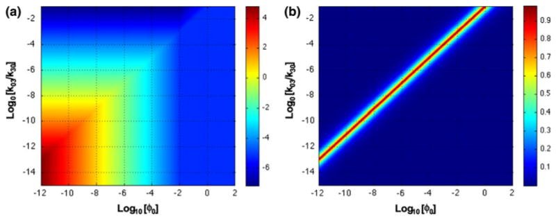
Discrimination and accuracy in system design space. (a) Discrimination between peptide bound to positive and negative tumors. The function Log₁₀(V₃X₃/(V₄X₄)) is plotted as a heat map on the z-axis. Red corresponds to high discrimination and blue to low. (b) Accuracy of X₃ determined from design space analysis. The function |X_3,Approx − X_3,Actual|/X_3,Actual is plotted as a heat map on the z-axis. See legend for Fig. 8.

The discrepancy between these results obtained from the design space analysis and those from the solution of the original equations are the largest along the diagonal border between regions 28 and 32 and regions 25 and 29, as can be seen from the difference plotted in Fig. 9b. Everywhere else, the results are nearly identical, and can be obtained much more easily from the analysis of the S-system approximation in each region. If we assume a low nominal value for the input (ϕ₀ = 10⁻¹⁰) and compare the discrimination ratio in response to variation in each of the parameters, then the results can be summarized as follows. There is essentially no change in discrimination ratio for changes in parameters related to tissue B in Fig. 7 (k₁₅, k₅₁, k_m5, V₅, k₀₆, k₆₀, T₆), for parameters related to the common part of tissue A (k₁₂, k₂₁, k_m2, V₂), and for the parameters of the central pool (k_e1, V₁). Discrimination is improved only in response to an increase or decrease in value of the remaining parameters. An improvement is observed for any increase in the parameters k₀₄ and T₃, and for an increase in k₃₀ up to a saturating value of 1000. Alternatively, an improvement is observed for any decrease in the parameters k₀₃, k₄₀ and T₄. Of these, the off rates (k₀₃ and k₀₄, the rate constants for dissociation of targets bound with labeled material) and the number of targets are probably the most significant parameters in practice.

A plot of discrimination as a function of the off rates for the specific and non-specific targets in tissue A (Fig. 10) suggests an explanation for the counterintuitive observation that compounds with high affinity for the specific target occasionally yield poorer discrimination than compounds with lower affinity.¹⁰ By comparing values of discrimination for the nominal compound (as shown in Fig. 10a with off rates of k₀₃ = 10⁻⁸ and k₀₄ = 10⁻³) with those for related compounds having alternative values that are assumed to be proportional (diagonal line in Fig. 10a), one can see that discrimination increases for compounds having lower affinity and decreases for those having higher affinity. This counterintuitive effect is eliminated when the input is much lower (ϕ₀ = 10⁻¹⁰), as shown in Fig. 10b.

FIGURE 10.

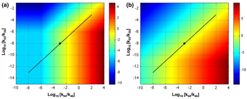
Discrimination as a function of equilibrium dissociation constants. The function Log₁₀(V₃X₃/(V₄X₄)) is plotted as a heat map on the z-axis for different values of the equilibrium dissociation constants k₀₃/k₃₀ on the y-axis for the specific target and k₀₄/k₄₀ on the x-axis for the non-specific target. Input (a) ϕ₀ = 10⁻⁵ and (b) ϕ₀ = 10⁻¹⁰. The black dot is the location of the operating point with the nominal values of the parameters given in Fig. 8. The diagonal line is the locus of alternative equilibrium dissociation constants if the values of the specific and non-specific constants of the test compound are proportional. See text for discussion.

Dynamic Discrimination

The dynamic responses that are the analog of the quasi-steady-state analysis in the previous section are show in Fig. 11. Before time zero the system is assumed to be in a steady state established with an input flux of peptide ϕ₀ = 100, and at time zero the infusion is stopped (or equivalently, at time zero there is an injection of a large bolus that is sufficient to saturate all targets). The labeled material then slowly leaves the system. The results with the nominal parameter values are shown in Fig. 11a. The dynamic discrimination at some intermediate time is better than expected on the basis of the quasi-steady state analysis, and is related to the large differences in off times for the specific and non-specific targets. These results are roughly comparable to the results of Gagnon et al.¹⁰ reproduced in Fig. 7, which show improved discrimination at 180 min after a bolus of peptide.

FIGURE 11.

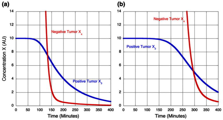
Time course for the concentration of peptide bound to specific and non-specific targets associated with positive and negative tumors. (a) Discrimination with the nominal concentration of non-specific targets (T₄ = 1.5 × 10⁶). (b) Discrimination with twice the nominal concentration of non-specific targets (T₄ = 3.0 × 10⁶). See text for discussion.

All the results in this section depend on the choice of parameter values, which can only be guesses at this point. The order of magnitude for the nominal values used above were estimated from data of Gagnon et al.¹⁰; more realistic values will require experiments specifically designed for the purpose. Indeed, the goal of modeling and analysis in this case is to make predictions that can guide experimental determination of the critical parameters.

The results are very sensitive to the concentration of non-specific targets, T₄, as shown in Fig. 11b. If the concentration of non-specific targets is increased by a factor of two, then the discrimination is nearly abolished at 180 min. The volumes V₃, V₄, and V₆ have no influence on the steady-state discrimination ratios because they do not appear in the steady-state equations. The dynamic discrimination between the positive and negative tumors in tissue B is not influenced by changes in the volume of targets in tissue A, V₆. The logarithmic gain of dynamic discrimination in response to a change in the volume of the targets for the positive tumor, V₃, is +0.1. For example, a 30-fold increase in volume results in an ∼3-fold increase in discrimination between the positive and negative targets. The logarithmic gain of dynamic discrimination in response to a change in the volume of the targets for the negative tumor, V₄, is −1. For example, a 10-fold decrease in volume results in an ∼10-fold increase in discrimination between the positive and negative targets.

The most sensitive parameters are the equilibrium dissociation constants (k_0i/k_i0) and the total amount of targets (concentration T_i times volume V_i). Thus, the results from both the steady-state and dynamic analyses can be roughly summarized in the following relationship for the best-case discrimination between positive and negative tumors:

$$D_{3.4}\approx \frac{k_3{k}_{04}{V}_3{T}_3}{k_4{k}_{03}{V}_4{T}_4}.$$

Tradeoffs

These results are consistent with the well-known tradeoffs associated with targeted molecular imaging. Higher input of targeting peptide yields the worst discrimination; lower input yields the best discrimination, but lower input means lower signal to noise ratio. At intermediate discrimination, the relative binding constants play a significant role. In some cases, a compound with a high binding constant for the specific target can yield the counterintuitive result that it provides less discrimination than a compound with a lower binding constant.¹⁰ As seen in Fig. 10, this can occur when a compound with tight binding to a few specific targets also has a marginal binding constant for many non-specific targets. The net result is an interplay among target sizes, binding constants, transport among pools, and metabolic clearance (proteolysis). With more accurate experimental estimates of the relevant parameters, and with corresponding model refinement, there is the possibility of making significant improvements in targeted therapies.

Membrane Protrusion of Migrating Cells

An application of a different type is based on the study of Welf and Haugh.³⁰ These authors formulated a conceptual model for the dynamics of membrane protrusion in migrating cells, proposed differential equations to represent the underlying processes, and performed stochastic simulations of the model behavior. Although mathematical modeling of the biomechanical aspects of cell adhesion and migration has received considerable attention,^1,8,16,17 few models have addressed the regulation of cell motility by coupling the mechanical aspects with the biochemical signaling pathways.^4,29 The following is an abbreviated summary of the conceptual model (Fig. 12) proposed by Welf and Haugh³⁰ in addressing this coupling.

FIGURE 12.

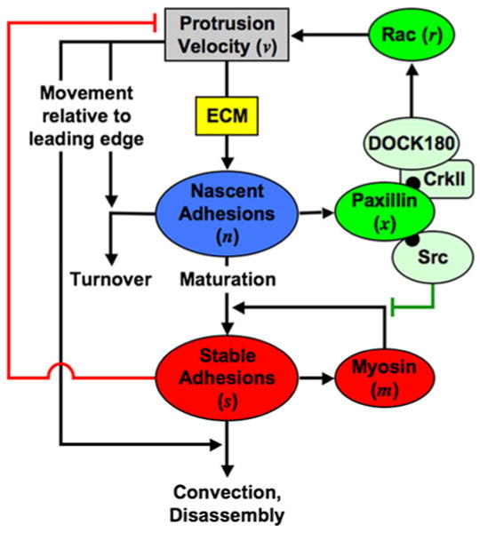
Conceptual model integrating biomechanical and biochemical aspects of membrane protrusion and cell migration. The spatial reference point for the model is the leading edge of a protruding region of the cell, and the modeled control volume represents the region directly behind the protruding edge, encompassing the lamellipodium and a portion of the lamella. See text for discussion. From Welf and Haugh.³⁰

Nascent adhesions (n) foster the activation of the small GTPase Rac (r). Active Rac in turn enhances the rate of protrusion of the cell's leading edge (v), which enhances the rate of nascent adhesion nucleation as a function the extracellular matrix (ECM); this feedback mechanism represents the core protrusion cycle. Nascent adhesions either turn over, at a rate that depends on the protrusion velocity, or they mature to form stable adhesions (s) under the influence of myosin (m) and a feedforward mechanism mediated by Src. Stable adhesions antagonize the rate of protrusion, so as to allow transient protrusion at higher densities of ECM, and disappear from the control volume either by disassembly or by rearward convection (which depends on protrusion velocity). Welf and Haugh show that the “buffering of inhibition” mechanism, coupled with the core protrusion cycle, is capable of tuning the frequencies of protrusion and adhesion maturation events.

Phenotypes from the Differential Equations

The nonlinear differential equations proposed by Welf and Haugh³⁰ for the system represented in Fig. 12 are

$$\begin{array}{c}\frac{dn}{dt}=k_{a,n}[1+E_{n}v]-k_{d,n}[1+C_{n}v]n-k_{a,s}\left[1+E_s\frac{m}{(1+I_{s}x)}\right]n\hfill \\ \frac{ds}{dt}=k_{a,s}\left[1+E_s\frac{m}{(1+I_{s}x)}\right]n-k_{d,s}[1+C_{s}v]s\hfill \\ \frac{dm}{dt}=k_{d,m}(s-m)\hfill \\ \frac{dx}{dt}=k_{d,x}{K}_{x}n-k_{d,x}{K}_{x}x-k_{d,x}x\hfill \\ \frac{dr}{dt}=k_{d,r}(x-r)\hfill \end{array}$$ (18)

where

$$v=\frac{K_{v}r}{(1+K_{v}r)(1+I_{n}s)}.$$

The corresponding steady-state equations can be recast into the following system of generalized mass-action equations in the power-law formalism ^22,24,25:

$$\begin{array}{c}0=k_{a,n}+k_{a,n}{E}_n{X}_6-k_{d,n}{X}_1-k_{d,n}{C}_n{X}_1{X}_6-X_{10}\hfill \\ 0=X_{10}-k_{d,s}{X}_2-k_{d,s}{C}_s{X}_2{X}_6\hfill \\ 0=X_2-X_3\hfill \\ 0=K_x{X}_1-K_x{X}_4-X_4\hfill \\ 0=X_4-X_5\hfill \\ 0=X_6-K_v{X}_5{X}_7^{-1}{X}_8^{-1}\hfill \\ 0=X_7-1-K_v{X}_5\hfill \\ 0=X_8-1-I_n{X}_2\hfill \\ 0=X_9-1-I_s{X}_4\hfill \\ 0=X_{10}-k_{a,s}{X}_1-k_{a,s}{E}_s{X}_1{X}_3{X}_9^{-1}\hfill \end{array}$$ (19)

where X₁ = n, X₂ = s, X₃ = m, X₄ = x, X₅ = r, and X₆ = v (protrusion velocity) are the fundamental variables in the original model, and X₇ through X₁₀ are auxiliary variables introduced in the recasting step by the following definitions:

$$X_7=1+K_v{X}_5,X_8=1+I_n{X}_2,X_9=1+I_s{X}_4,X_{10}=k_{a,s}\left[1+E_s\frac{m}{(1+I_{s}x)}\right]n.$$

A bound, T, on the total number of qualitatively distinct phenotypic regions in this case is 384 (or 192 when K_x = 1.0, as in Welf and Haugh,³⁰ and the fourth of Eq. (19) is written as 0 = X₁ − 2X₄).

Welf and Haugh³⁰ estimated the model parameters based on experimental evidence where possible and systematically varied parameters to determine their effect on protrusion and adhesion dynamics. Assuming their nominal values for parameters yields the system design space in Fig. 13 with only seven valid regions.

FIGURE 13.

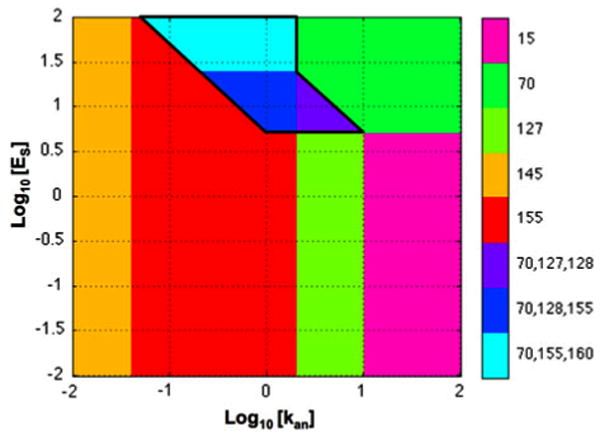
System design space for the system in Fig. 12. The x-axis represents the density and character of the extracellular matrix, k_an; the y-axis represents the enhancement of adhesion maturation by myosin, E_s. The nominal values of the parameters are the following: k_an = 1, k_d,n = 0.1, k_a,s = 0.01, k_d,s = 0.1, k_d,x = 10, k_d,r = 4, k_d,m = 4, E_n = 100, C_n = 20, E_s = 100, C_s = 100, K_v = 1, K_x = 1, I_n = 10, I_s = 1.

The regions associated with three Case numbers have the signature of hysteretic bistability (see also Savageau and Fasani^23,24). In these regions there are two stable steady states and one saddle-point instability. For clarity, the Cases representing saddle-point instability are shown as isolated regions in Fig. 14.

FIGURE 14.

Regions representing saddle-point instability. (a) Case 150, (b) Case 160, and (c) Case 128. See legend of Fig. 13 for details.

Local Analysis of the Steady States in a Region of Overlapping Cases

The ease with which one can analyze the dominant S-system equations will be illustrated in the treatment of a region with overlapping cases. The following makes use of well-established methods for analyzing the local behavior of nonlinear S-system equations.^22,21 The system design space methodology²⁵ yields the dominant S-system equations for each of the cases. Except for three cases in Fig. 14, all of the cases exhibit a locally stable steady state. An example of the three cases that overlap in a given region is the following.

Case 70	Case 155	Case 160
$\frac{dn}{dt}=k_{an}-0.01E_{s}nm$	$\frac{dn}{dt}=100k_{an}-2n$	$\frac{dn}{dt}=10k_{an}{s}^{-1}-0.2n{s}^{-1}$
$\frac{ds}{dt}=0.01E_{s}nm-0.1s$	$\frac{ds}{dt}=0.01n-10s$	$\frac{ds}{dt}=0.01E_{s}nm{x}^{-1}-1$
$\frac{dm}{dt}=4s-4m$	$\frac{dm}{dt}=4s-4m$	$\frac{dm}{dt}=4s-4m$
$\frac{dx}{dt}=10n-20x$	$\frac{dx}{dt}=10n-20x$	$\frac{dx}{dt}=10n-20x$
$\frac{dr}{dt}=4x-4r$	$\frac{dr}{dt}=4x-4r$	$\frac{dr}{dt}=4x-4r$

The steady-state solutions for values of k_an = 1 and E_s = 50 (within the region of overlapping cases) are obtained in general by a logarithmic transformation and solution of the resulting linear equations.

Case 70	Case 155	Case 160
$n=2x=10/E_s=0.2$	$n=2x=50k_{an}=50$	$n=2x=10k_{an}/0.2=50$
$s=m=500k_{an}/E_s=10$	$s=m=0.001n=0.05$	$s=m=100/(2E_s)=1$
$r=x=n/2=0.1$	$r=x=n/2=25$	$r=x=n/2=25$
$v=0.000900$	$v=0.641$	$v=0.0874$

The pseudo first-order rate constants for the linearized equations are given by

Case 70	Case 155	Case 160
$F_1=0.5nm/n=5$	$F_1=2n/n=2$	$F_1=0.2n{s}^{-1}/n=0.2$
$F_2=0.1s/s=0.1$	$F_2=10s/s=10$	$F_2=1/s=1$
$F_3=4m/m=4$	$F_3=4m/m=4$	$F_3=4m/m=4$
$F_4=20x/x=20$	$F_4=20x/x=20$	$F_4=20x/x=20$
$F_5=4r/r=4$	$F_5=4r/r=4$	$F_5=4r/r=4$

The linearized S-system equations are then

Case 70	Case 155	Case 160
$\frac{d{u}_1}{dt}=F_1[-u_1-u_3]$	$\frac{d{u}_1}{dt}=F_1[-u_1]$	$\frac{d{u}_1}{dt}=F_1[-u_1]$
$\frac{d{u}_2}{dt}=F_2[u_1-u_2+u_3]$	$\frac{d{u}_2}{dt}=F_2[u_1-u_2]$	$\frac{d{u}_2}{dt}=F_2[u_1+u_3-u_4]$
$\frac{d{u}_3}{dt}=F_3[u_2-u_3]$	$\frac{d{u}_3}{dt}=F_3[u_2-u_3]$	$\frac{d{u}_3}{dt}=F_3[u_2-u_3]$
$\frac{d{u}_4}{dt}=F_4[u_1-u_4]$	$\frac{d{u}_4}{dt}=F_4[u_1-u_4]$	$\frac{d{u}_4}{dt}=F_4[u_1-u_4]$
$\frac{d{u}_5}{dt}=F_5[u_4-u_5]$	$\frac{d{u}_5}{dt}=F_5[u_4-u_5]$	$\frac{d{u}_5}{dt}=F_5[u_4-u_5]$

The characteristic equations follow directly from the linearized S-system equations.

Case 70

$$(\lambda +F_4)(\lambda +F_5)[{\lambda }^3+(F_1+F_2+F_3){\lambda }^2+(F_1{F}_2+F_1{F}_3)\lambda +F_1{F}_2{F}_3]=0.$$

Application of the Routh criteria for stability shows that there are no roots with positive real part, no matter what the values are for the F-factors. Thus, this subsystem is locally stable throughout the region.

Case 155

$$(\lambda +F_1)(\lambda +F_2)(\lambda +F_3)(\lambda +F_4)(\lambda +F_5)=0.$$

By inspection, this subsystem also is stable, no matter what the values are for the F-factors, and thus is stable throughout the region.

Case 160

$$(\lambda +F_1)(\lambda +F_4)(\lambda +F_5)[{\lambda }^2+F_3\lambda -F_2{F}_3]=0.$$

This subsystem has one positive real root, which indicates asymptotic instability. Again, this is true for all values of the F-factors, and thus it is true throughout the region.

Comparison of Results

Welf and Haugh showed that the interplay between Src-mediated inhibition of adhesion maturation (I_s) and adhesion-mediated inhibition of protrusion (I_n) controls protrusion/adhesion dynamics. With I_n ≥ I_s, the full diversity of their dynamics was reproduced at low ECM density (k_an), but not at high density. One can display any of the system properties region by region on the z-axis in the system design space. Figure 15 shows two examples that can be compared with the analogous results in Fig. 16 from Welf and Haugh (personal communication). In both cases, there are sustained stable adhesions at high density of ECM (k_an > 1) and high values of adhesion maturation (E_s > 10), and with only rare transient protrusions in the stochastic simulations. It should be emphasized that Fig. 15 represents the results from the deterministic equations, whereas Fig. 16 represents the results from stochastic simulations based on the same equations. In addition, there is some ambiguity in the coloring of regions with overlapping cases in Fig. 15; although the values for the unstable steady state are not represented, one must decide which of the two stable steady-state values to plot.

FIGURE 15.

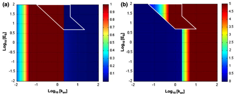
Steady-state values of protrusion rate and stable adhesions from the deterministic model. (a) Protrusion rate, v, and (b) stable adhesions, s, represented as a heat map on the z-axis of the system design space. In the region of overlapping cases, the values are plotted for the steady state with the largest values. See legend of Fig. 13 for details.

FIGURE 16.

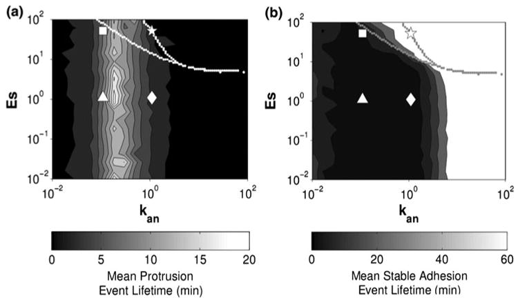
Mean lifetimes of protrusion and stable adhesion events from the stochastic model.³⁰ (a) Protrusion, v, and (b) stable adhesions, s, represented as a heat map on the z-axis. At high density of ECM (k_an = 1) and myosin-mediated maturation of adhesions (E_s = 50), sustained stable adhesions were observed with only rare transient protrusions. The dashed lines represent the region of hysteretic behavior as revealed by bifurcation analysis. From Welf and Haugh (personal communication).

The location of the bistability region in Fig. 16, which is obtained from conventional bifurcation analysis, differs from that in Fig. 15, which is obtained from the design space methodology. This is not surprising, given the aim of design space analysis, which is to identify, enumerate, and characterize the qualitatively distinct phenotypic repertoire of a model. It is not expected to accurately represent the quantitative behavior. Some of the boundaries in the system design space correspond to conventional bifurcations, but many of the others do not. Moreover, the boundaries representing the region of hysteresis typically overestimate these regions, as in this case as well as in the case of the classic lactose gene circuit,²³ so interpretation of the situation near these boundaries requires special care.

In contrast to the results shown in Figs. 15 and 16, when I_n = 1 and I_s = 10 the full diversity of protrusion/adhesion dynamics was reproduced at both low and high ECM density.³⁰ The results for protrusion velocity are very similar to those in Figs. 15a and 16a with a band of high protrusion velocity centered around values of k_an between 0.3 and 1.0; however, the results for stable adhesions corresponding to Figs. 15b and 16b show essentially a vertical boundary with low values to the left of k_an values between 2 and 20 (data not shown). Similar results were found when I_n = 10 and I_s = 100, showing that it is the ratio of the inhibition of adhesion maturation (I_s) to the adhesion-mediated inhibition of protrusion (I_n) that is important for tuning the system to achieve appropriate transient protrusions even at high density of ECM.³⁰

Conclusions

We have used the example in Fig. 1 to introduce the concepts of system design space and qualitatively distinct phenotype at the level of a molecular system. This simple example exhibits some of the subtle issues connected with the construction of the system design space. For example, this case leads to a singular S-system with a particular case of dominance. With appropriate care, these cases can be resolved by reformulating the original equations, as we have seen. In other cases one can on occasion obtain a completely blank space because of a unique set of nominal values for the parameters. This is analogous to being on a boundary (knife edge). In these cases, one can simply add an infinitesimal value to the parameters and the issue is overcome. These two types of issues are understood and relatively easy to resolve. Nevertheless, the system design space methodology is still undergoing development and there could well be other issues that might arise in future applications.

The utility of these concepts is not restricted to simple systems such as that in Fig. 1. In general, the repertoire of qualitatively distinct phenotypes is much larger and the system design space is accordingly more complex, as was seen in the example of the previous section. The examples of biomedical engineering interest are intended to suggest strategies for qualitative analysis using the system design space methodology without performing a full analysis, which would be beyond the space of this review.

The system design space has been constructed for other examples of elementary motifs found in metabolic networks, including pathways,²⁵ moiety-transfer cycles,^5,6 and branch-points.²⁵ System design spaces also have been constructed for gene circuits involving local²³ as well as global²⁸ regulators, recombination events in gene duplications,¹⁹ and the developmental switch in a temperate virus.²⁴ In each case, when the local analysis of all regions is taken into account, one obtains a fairly complete characterization of the qualitatively distinct repertoire. For example, the local characterization of overlapping regions that reveals hysteretic bistability provides insight into global behavior as well. However, in general, large-scale dynamic behavior—that which involves transit through several regions—is still an open question. It certainly can be explored computationally by doing piecewise continuous simulations through the regions. This is one of the areas that are still being explored.

In general, the boundaries in the system design space are always straight lines (hyper planes) in logarithmic space and the slopes are rational functions of the exponents in generalized mass action models. Algebraic geometry provides the theoretical foundation for this type of analysis and there are opportunities for automating much of the analysis based on this linear theory. Indeed, a set of algorithms have been developed and assembled into a Matlab application called Design Space Toolbox,⁹ and there is the potential for further automation. For example, establishing dominance is a standard mathematical problem in linear algebra that is solved everyday for problems of enormous size (e.g., scheduling in the airline industry), so that solving each case is not a problem. Nevertheless, scale up becomes an issue because of the large number of potential phenotypes, which is determined by the number of combinations of terms in the original equations, many of which will be invalid but still must be checked. This is an obviously parallizable problem yet to be implemented. As should be clear from these conclusions, the analysis of system design space is in its infancy and there are still abundant challenges and opportunities for further development.

References

- 1.Bershadsky AD, Ballestrem C, Carramusa L, Zilberman Y, Gilquin B, et al. Assembly and mechanosensory function of focal adhesions: experiments and models. Eur J Cell Biol. 2006;85:165–173. doi: 10.1016/j.ejcb.2005.11.001. [DOI] [PubMed] [Google Scholar]
- 2.Brenner S. Genomics: the end of the beginning. Science. 2000;287:2173–2174. doi: 10.1126/science.287.5461.2173. [DOI] [PubMed] [Google Scholar]
- 3.Carson ER, Cobelli C. Modeling Methodology for Physiology and Medicine. San Diego: Academic Press; 2001. [Google Scholar]
- 4.Cirit M, Krajcovic M, Choi CK, Welf ES, Horwitz AF, Haugh JM. Stochastic model of integrin-mediated signaling and adhesion dynamics at the leading edges of migrating cells. PLoS Comput Biol. 2010;6:e1000688. doi: 10.1371/journal.pcbi.1000688. [DOI] [PMC free article] [PubMed] [Google Scholar]
- 5.Coelho PMBM, Salvador A, Savageau MA. Global tolerance of biochemical systems and the design of moiety-transfer cycles. PLoS Comput Biol. 2009;5(3):e1000319. doi: 10.1371/journal.pcbi.1000319. [DOI] [PMC free article] [PubMed] [Google Scholar]
- 6.Coelho PMBM, Salvador A, Savageau MA. Relating genotype to phenotype via the quantitative behavior of the NADPH redox cycle in human erythrocytes: mutant analysis. PLoS One. 2010;5(9):e13031. doi: 10.1371/journal.pone.0013031. [DOI] [PMC free article] [PubMed] [Google Scholar]
- 7.Daun S, Rubin J, Vodovotz Y, Roy A, Parker R, Clermont G. An ensemble of models of the acute inflammatory response to bacterial lipopolysaccharide in rats: results from parameter space reduction. J Theor Biol. 2008;253:843–853. doi: 10.1016/j.jtbi.2008.04.033. [DOI] [PubMed] [Google Scholar]
- 8.Deshpande VS, McMeeking RM, Evans AG. A bio-chemo-mechanical model for cell contractility. Proc Natl Acad Sci USA. 2006;103:14015–14020. doi: 10.1073/pnas.0605837103. [DOI] [PMC free article] [PubMed] [Google Scholar]
- 9.Fasani RA, Savageau MA. Design Space Toolbox: a Matlab application for construction of the design space for molecular systems and analysis of their qualitatively distinct phenotypes. Bioinformatics. 2010;26:2601–2609. doi: 10.1093/bioinformatics/btq479. [DOI] [PMC free article] [PubMed] [Google Scholar]
- 10.Gagnon MKJ, Hausner SH, Marik J, Abbey CK, Marshall JF, Sutcliffe JL. High-throughput in vivo screening of targeted molecular imaging agents. Proc Natl Acad Sci USA. 2009;106:17904–17909. doi: 10.1073/pnas.0906925106. [DOI] [PMC free article] [PubMed] [Google Scholar]
- 11.Geysen HM, Schoenen F, Wagner D, Wagner R. Combinatorial compound libraries for drug discovery: an ongoing challenge. Nat Rev Drug Discov. 2003;2:222–230. doi: 10.1038/nrd1035. [DOI] [PubMed] [Google Scholar]
- 12.Gutenkunst RN, Waterfall JJ, Casey FP, Brown KS, Myers CR, et al. Universally sloppy parameter sensitivities in systems biology models. PLoS Comput Biol. 2007;3:1871–1878. doi: 10.1371/journal.pcbi.0030189. [DOI] [PMC free article] [PubMed] [Google Scholar]
- 13.Hausner SH, DiCara D, Marik J, Marshall JF, Sutcliffe JL. Use of a peptide derived from foot-and-mouth disease virus for the noninvasive imaging of human cancer: generation and evaluation of 4-[18F]fluorobenzoyl A20FM DV2 for in vivo imaging of integrin αvβ6 expression with positron emission tomography. Cancer Res. 2007;67:7833–7840. doi: 10.1158/0008-5472.CAN-07-1026. [DOI] [PubMed] [Google Scholar]
- 14.Hlavacek WS. How to deal with large models? Mol Syst Biol. 2009;5:240–242. doi: 10.1038/msb.2008.80. [DOI] [PMC free article] [PubMed] [Google Scholar]
- 15.Lam KS, Lebl M, Krchnak V. The “one-bead-one-compound” combinatorial library method. Chem Rev. 1997;97:411–448. doi: 10.1021/cr9600114. [DOI] [PubMed] [Google Scholar]
- 16.Mogilner A. Mathematics of cell motility: have we got its number? J Math Biol. 2009;58:105–134. doi: 10.1007/s00285-008-0182-2. [DOI] [PMC free article] [PubMed] [Google Scholar]
- 17.Novak IL, Slepchenko BM, Mogilner A, Loew LM. Cooperativity between cell contractility and adhesion. Phys Rev Lett. 2004;93:268109. doi: 10.1103/PhysRevLett.93.268109. [DOI] [PubMed] [Google Scholar]
- 18.Qi J, Leahy RM, Cherry SR, Chatziioannou A, Farquhar TH. High-resolution 3D Bayesian image reconstruction using the microPET small-animal scanner. Phys Med Biol. 1998;43:1001–1013. doi: 10.1088/0031-9155/43/4/027. [DOI] [PubMed] [Google Scholar]
- 19.Reams AB, Kofoid E, Savageau MA, Roth JR. Duplication frequency in a population of Salmonella enterica rapidly approaches steady state with or without recombination. Genetics. 2010;184:1077–1094. doi: 10.1534/genetics.109.111963. [DOI] [PMC free article] [PubMed] [Google Scholar]
- 20.Riviere JE. Comparative Pharmacokinetics: Principles, Techniques and Applications. Ames, IA: Iowa State University Press; 1999. [Google Scholar]
- 21.Savageau MA. Reading, MA: Addison-Wesley; 1976. Biochemical Systems Analysis: A Study of Function and Design in Molecular Biology. 40th Anniversary Edition, A reprinting of the original edition, 2009, http://www.amazon.com/Biochemical-Systems-Analysis-Function-Molecular/dp/1449590764/ [Google Scholar]
- 22.Savageau MA. Design principles for elementary gene circuits: elements, methods, and examples. Chaos. 2001;11:142–159. doi: 10.1063/1.1349892. [DOI] [PubMed] [Google Scholar]
- 23.Savageau MA. Design of the lac gene circuit revisited. Math Biosci. 2010 doi: 10.1016/j.mbs.2011.03.008. in press. [DOI] [PMC free article] [PubMed] [Google Scholar]
- 24.Savageau MA, Fasani RA. Qualitatively distinct phenotypes in the design space of biochemical systems. FEBS Lett. 2009;583:3914–3922. doi: 10.1016/j.febslet.2009.10.073. [DOI] [PMC free article] [PubMed] [Google Scholar]
- 25.Savageau MA, Coelho PMBM, Fasani R, Tolla D, Salvador A. Phenotypes and tolerances in the design space of biochemical systems. Proc Natl Acad Sci USA. 2009;106:6435–6440. doi: 10.1073/pnas.0809869106. [DOI] [PMC free article] [PubMed] [Google Scholar]
- 26.Sutcliffe-Goulden JL, et al. Rapid solid phase synthesis and biodistribution of 18F-labeled linear peptides. Eur J Nucl Med Mol Imaging. 2002;29:754–759. doi: 10.1007/s00259-001-0756-3. [DOI] [PubMed] [Google Scholar]
- 27.Tai YC, et al. Performance evaluation of the microPET focus: a third-generation microPET scanner dedicated to animal imaging. J Nucl Med. 2005;46:455–463. [PubMed] [Google Scholar]
- 28.Tolla DA, Savageau MA. Phenotypic repertoire of the FNR regulatory network in Escherichia coli. Mol Microbiol. doi: 10.1111/j.1365-2958.2010.07437.x. [DOI] [PMC free article] [PubMed] [Google Scholar]
- 29.Vogel V, Sheetz M. Cell fate regulation by coupling mechanical cycles to biochemical signaling pathways. Curr Opin Cell Biol. 2009;21:38–46. doi: 10.1016/j.ceb.2009.01.002. [DOI] [PMC free article] [PubMed] [Google Scholar]
- 30.Welf ES, Haugh JM. Stochastic dynamics of membrane protrusion mediated by the DOCK180/Rac pathway in migrating cells. Cell Mol Bioeng. 2010;3:30–39. doi: 10.1007/s12195-010-0100-8. [DOI] [PMC free article] [PubMed] [Google Scholar]