From Neural Arbors to Daisies

Abstract

Pyramidal neurons in layers 2 and 3 of the neocortex collectively form an horizontal lattice of long-range, periodic axonal projections, known as the superficial patch system. The precise pattern of projections varies between cortical areas, but the patch system has nevertheless been observed in every area of cortex in which it has been sought, in many higher mammals. Although the clustered axonal arbors of single pyramidal cells have been examined in detail, the precise rules by which these neurons collectively merge their arbors remain unknown. To discover these rules, we generated models of clustered axonal arbors following simple geometric patterns. We found that models assuming spatially aligned but independent formation of each axonal arbor do not produce patchy labeling patterns for large simulated injections into populations of generated axonal arbors. In contrast, a model that used information distributed across the cortical sheet to generate axonal projections reproduced every observed quality of cortical labeling patterns. We conclude that the patch system cannot be built during development using only information intrinsic to single neurons. Information shared across the population of patch-projecting neurons is required for the patch system to reach its adult state.

Introduction

The neocortex holds a significant advantage over any man-made device as a computationally powerful and energy-efficient information processing system (Laughlin and Sejnowski 2003) and displays exquisite structural complexity in the ramifications of axonal and dendritic arbors of the neurons that compose it (Gilbert and Wiesel 1979; Ramón y Cajal 1989). Despite these heights of intricacy at the scale of single neurons and wide-ranging feats of function at a system level, the cortex nevertheless shows surprising regularity in its repeated motifs of network design (Gilbert 1983; Douglas and Martin 2004).

The “superficial patch system” (also known as the “daisy architecture”—Douglas and Martin 2004) is one such motif. Upon injecting the neural tracer horseradish peroxidase (hrp) into the primary visual cortex of the tree shrew, Rockland and Lund (1982) described a series of bands or “patches” of dense label transported from the injection site, separated by regions of weak or absent label. Although originally observed in tree shrew visual cortex, the patch system is by no means confined to a single species or cortical area and has since been observed widely across cortex and in many other animals: cat area 17 (Gilbert and Wiesel 1983) and A1 (Wallace et al. 1991); macaque monkey V1 (Rockland and Lund 1983), V2 (Rockland 1985a), motor (Huntley and Jones 1991), IT (Fujita 2002), and prefrontal cortex (Lewis et al. 2002); ferret area 17 (Rockland 1985b) and A1 (Wallace and Bajwa 1991); prosimian galago V1 (Cusick and Kaas 1988b); human V1 and V2 (Burkhalter and Bernardo 1989); owl monkey MT (Malach et al. 1997); marsupial quokka area 17 (Tyler et al. 1998), and so on. The universality of this system suggests that it can be adapted to many tasks and forms part of the fundamental substrate for cortical computation.

The precise circuitry underlying the patch system remains unknown, but it is commonly assumed that labeled patches are composed of the clustered axonal projections arising from pyramidal cells in the superficial layers, which spread for several millimeters within a single cortical area (Rockland and Lund 1982; Rockland et al. 1982; Gilbert and Wiesel 1983; Rockland and Lund 1983; Price 1986; Callaway and Katz 1990; Yoshioka et al. 1992, 1996). Reconstructions of axonal arbors arising from small numbers of colabeled pyramidal cells in cat visual cortex show that despite the highly anisotropic and individual nature of each arbor, patch-projecting neurons collaborate to produce the population-scale labeling patterns (Kisvárday and Eysel 1992; Buzás et al. 2006). However, the rules that govern the convergence of axonal arbors to form the superficial patch system remain unknown. We tested candidate sets of geometric rules for generating individual axonal arbors for their ability to collectively form clustered labeling patterns, by simulating bulk injections of tracers into fields of generated neurons. The success or failure of rule sets provides constraints on what information must be shared among neurons during arbor growth to build the superficial patch system, indicating what kinds of information must be available to neurons in cortex during development.

Observed Patterns of Clustered Labeling In Vivo

Several aspects of the labeling patterns that form the primary description of the superficial patch system are not easily explained. Here we list experimental observations that will be not be used to define out models but will be used as criteria for successful modeling.

The first difficulty is that the size of a labeled patch never exceeds some maximum size in a given cortical area (observation A). Large injections (greater than the average patch diameter for that cortical area) result in patches of labeled cortex with the same width and spacing as small injections (Rockland and Lund 1982, 1983; Rockland et al. 1982; Lund et al. 2003). The fact that large injections result in discrete clusters of label at all is surprising, when one considers the functional properties of primary visual cortex. In this and other cortical areas, labeled patches connect regions of cortex with similar functional properties (“like-to-like” connectivity; a phrase coined by Mitchison and Crick [1982] to propose that patch system projections should connect neurons of similar functional properties. Connectivity between small regions of cortex with similar functional properties has been demonstrated for several species and cortical areas [Lund et al. 2003]). However, functional properties such as orientation preference are arranged quasi-periodically across the surface of primary visual cortex, in a manner that provides uniform coverage of the cortical surface (Swindale et al. 2000; Bosking et al. 2002). The combination of periodic functional maps and like-to-like patch connections would seem to suggest that a large injection covering all phases of orientation preference should uniformly label visual cortex, in conflict with observed labeling patterns. Any complete model of the patch system must resolve this conflict.

Although discrete patch size is largely independent of injection diameter, very large injections in visual cortex nevertheless reveal a qualitatively different pattern in the patch system. In at least tree shrew, primate, and quokka, large pressure injections result in a lattice work of labeling immediately surrounding the injection site, composed of walls of labeled terminals and somata surrounding “lacunae” of relatively unlabeled tissue (observation B—Rockland et al. 1982; Rockland and Lund 1983; Tyler et al. 1998; illustrated in Fig. 1a,b). With increasing distance from the injection site, this lattice work breaks up into separately labeled patches of the characteristic size for the cortical area that contains them. Retrogradely labeled somata are observed within the lattice walls and not within lacunae. Cytochrome oxidase–reactive regions (CO blobs) also fall within the lattice walls and avoid lacunae (Rockland and Lund 1983).

Figure 1.

Horizontal projections in monkey and rodent area 17. Highlighted regions in (b) and (d) indicate significantly anisotropic labeling (P < 0.01), as determined by our cluster-seeking density analysis, produced by injections of bidirectional (a; monkey, Rockland and Lund 1983) and retrograde tracers (c; gray squirrel, Van Hooser et al. 2006). See Figure S1 for more details of the cluster identification process. (a and b) Reveal the patchy and lattice-like structure of labeling in primate V1. While retrograde labeling in the rodent shows some anisotropy (highlighted areas in d), it does not display the extensive lattice of label nor the periodic clustering observed in the primate. (a) Reprinted from Rockland and Lund (1983), with permission of Wiley-Liss, Inc., a subsidiary of John Wiley & Sons, Inc. (b) Reproduced from (Van Hooser et al. 2006) with permission from HighWire Press. Scale bars: 500 μm.

Observations of retrogradely labeled somata located within labeled patches of axonal segments (e.g., fig. 2 of Angelucci et al. 2002b; fig. 7 of Tyler et al. 1998; Rockland et al. 1982; Rockland and Lund 1983) indicate that projections are patch reciprocal over a set of labeled patches (observation C). However, the origin of these labeled axonal segments is confused precisely by the bidirectional labeling present in these observations. Since the local axonal arbor of a neuron usually forms the densest cluster (Binzegger et al. 2007), it is possible that most of the labeled axonal segments surrounding a group of retrogradely labeled somata arises from exactly those somata, rather than from neurons labeled at the injection site. Nevertheless, reconstructions of small numbers of neurons participating in a set of patches (Kisvárday and Eysel 1992) reveal a striking degree of patch recurrence, as well as a propensity for colabeled neurons to send projections to similar regions of cortex.

Assumed Properties of the Superficial Patch System

In the absence of a deep understanding of the superficial patch system, and in the face of conflicting and equivocal descriptions of the system, various simplifying and clarifying assumptions must be made to construct our models.

As mentioned in the introduction, we assume the clustered nature of population-level labeling patterns to be a direct consequence of the clustered intrinsic axonal arbors of superficial layer pyramidal cells (assumption 1—Mitchison and Crick 1982; Rockland and Lund 1982; Gilbert and Wiesel 1983; Callaway and Katz 1990; Kisvárday and Eysel 1992; Bosking et al. 1997; see the third paragraph of the Introduction).

We assume that the patch system is roughly periodic (assumption 2). While this seems to be more true for primary sensory areas than for higher areas in the visual hierarchy (Amir et al. 1993; Malach et al. 1997; Tanigawa et al. 2005) or for prefrontal cortex (Levitt et al. 1993; Lund et al. 1993; Lewis et al. 2002), we assume for this set of models that similar geometric mechanisms underlie the structure of the patch system in all cortical areas.

The smoothly changing nature of functional maps in visual cortex, coupled with the like-to-like connection bias of the superficial patch system, suggests that two slightly offset injections into adjacent locations in cortex should produce labeled clusters with a similar spatial offset (assumption 3—Lund et al. 2003).

Although the granular and subgranular layers of cortex also display poorly understood patterns of clustered projections (Rockland 1985a; Yoshioka et al. 1992; Asi et al. 1996; Galuske and Singer 1996; Lund et al. 2003; Shmuel et al. 2005; Angelucci and Sainsbury 2006), we assume that the clustered intrinsic arbors within the superficial layers are sufficient to reveal what is usually referred to as the superficial patch system (assumption 4). This assumption is justified by the observation that the axonal arbors of ten superficial layer pyramidal cells labeled from a single injection is already sufficient to reveal evidence of a periodic projection structure (Kisvárday and Eysel 1992). We also assume that isotropic arbors of other cells in cortex (i.e., isotropic dendritic and axonal arbors of inhibitory and other inter-neurons) do not contribute to the clustered nature of the system.

We assume that tracer uptake and transport is independent of activity and that activity during the labeling process is not required to reveal the patch system (assumption 5). Since the time course of tracer transport is much longer than that of neural activity, we assume that any independent clustered patterns of activity within a cortical area will occur with uniform probability while transport occurs.

We assume that the visibility of the patch system is not dependent on some neurons being more intensely labeled than others; we assume that for most injections, “labeled neurons” are completely and equally well labeled (assumption 6). We do allow multiple boutons and somata to be labeled at discrete locations in space, which can produce more dense labeling at some locations than others by virtue of the labeling of a greater number of discrete elements. We also make the simplifying assumption that the uptake of tracer is uniform within an injection site (assumption 7). Nonuniform tracer uptake artificially increases the degree of clustered labeling following simulated injections; by enforcing uniform tracer uptake, our models must explain clustered labeling solely through patterns of axonal projection.

It is believed that patch-projecting neurons exist at most points in cortex and that a small injection into cortex will almost always result in clustered labeling (assumption 8—Lund et al. 2003). The obligatory exception to this rule, for primary visual cortex, is revealed by small injections into the centers of orientation-preference pinwheels. Anterograde (transport of tracer from the soma toward the distal neurites) and retrograde (transport from distal neurites toward the soma) labeling from injections made into these singularities displays no evidence of clustered projections, indicating that at least some regions of cortex do not participate in the patch system (assumption 9—Sharma et al. 1995; Yousef et al. 2001; Mariño et al. 2005).

Livingstone and Hubel (1984a) noted that when they made large injections into squirrel monkeys, the most distal labeled patches always fell inside regions of elevated cytochrome oxidase activity (CO blobs) in the superficial layers of monkey visual cortex, later confirmed for human (Burkhalter and Bernardo 1989), and prosimian visual cortex (Cusick and Kaas 1988b). Rockland and Lund (1983) saw no such relationship between CO domains and the farthest patches labeled in macaque visual cortex. Instead, they commented that the lattice work of label closely surrounding large injections seems to prefer CO blobs—regions of CO activity always fell within the labeled walls of the lattice and not in the poorly labeled lacunae (observation B above—Rockland and Lund 1983). The observation by Livingstone and Hubel implies that neurons in CO blobs make longer axonal projections than neurons elsewhere across the cortical surface. We therefore permit that some small regions of our simulated cortex make longer axonal projections than elsewhere (assumption 10).

Previous Models of Patchy Connectivity

Early experimentalists, observing the periodic clusters of labeled and unlabeled tissue that resulted from large injections of tracer, concluded that there must be two projection systems in visual cortex: zones which make periodic, reciprocal clustered projections over large distances within a cortical area, separated by zones of only local connectivity (Rockland and Lund 1982; Rockland et al. 1982).

As a response to these proposals for a compartmentalization of cortex into several nonoverlapping projection systems, Mitchison and Crick (1982) proposed a single-compartment model based on preferential connectivity between neurons of similar function. In addition to defining a hard “like connects to like” constraint (and coining the phrase in the process), they also proposed that the physical direction taken by axonal projections across cortex was defined by the functional preference of that neuron. Coupled with a simple model of an orientation map, their model predicted stripes of label for both small and large injections of tracer but cannot predict the nonpatchy labeling patterns seen following pinwheel injections. A modern take on this model was recently proposed by Buzás et al. (2006), who however removed Mitchison and Crick's bias on projection direction from their model. As a result, an injection into a functional domain produces a patchy field with more or less isotropic spread around the injection site. As the injection site expands, so each distant labeled patch expands to label adjacent functional domains; once an injection site covers all phases of function, their model will produce a uniform field of label and will not predict discrete patches of label from large injections.

It is unclear how models of the patch system based on functional maps of visual cortex relate to other areas of cortex, where our knowledge of their respective functional arrangements is either scant or entirely absent. We also note with interest the developmental time scale of the superficial patch system (Price 1986; Callaway and Katz 1990; Durack and Katz 1996; Ruthazer and Stryker 1996). Since the system is visible in visual cortex in a coarse form before the afferents carrying structured activity arrive in the superficial layers, we infer that the patch system can exist independent of any imposed functional modality. For these reasons, the models we describe in this paper do not rely directly on the function of any particular area of cortex.

Voges et al. (2010) had a different take on the properties of patchy networks. They asked what effect long distance connections, with various configurations, had on the signal transmission and graph statistical properties of a network. They briefly examined the patterns of labeling formed by point injections into their networks, without attempting to replicate labeling patterns observed in cortex. Their models have a more spatially random flavor than those discussed in this paper, and only one (their “overlapping patches” model) incorporates periodic patch locations.

Aside from the central prediction of patterned labeling resulting from most small injections of tracer, a model must explain several other phenomena to be successful. Large simulated injections must produce a lattice work of label (observation B), but the upper size of discrete patches must be limited (observation A). Injections of bidirectional tracers must yield colocated patches of labeled axonal segments and somata (observation C). Finally, small injections into “pinwheel-like” regions must result in non-patterned labeling (assumption 9). We present several models for the superficial patch system, incrementally examining each of these phenomena and their relationship to axonal projection rules for cortical neurons.

Materials and Methods

By making simulated injections of tracers into 2D fields of neurons, with axonal arbors formed by prescribed geometric rules, we attempted to reproduce the labeling patterns of the superficial patch system. In this way, we eliminated rules for axonal arbors that do not reproduce the structured labeling patterns described above. Briefly, we built geometric models describing how individual pyramidal neurons form clustered arborizations within an area of cortex. Fields of these generated neural arbors were composed into a sheet representing the superficial layers of cortex. Simulated injections of antero- and retrograde—as well as bidirectional—tracers produced labeling patterns which we compared against the observed patterns of the superficial patch system. Depending on the assumptions underlying each model, we could reproduce some or all the observed features of clustered labeling in cortex.

In the following sections, we describe the mechanics of our models in detail.

Density Estimation and Patch Delineation

The majority of reconstructions of patch locations in the literature have used the highly subjective technique of delineating patches by eye (e.g., Rockland et al. 1982; Cusick and Kaas 1988a; Juliano et al. 1990; Boyd and Matsubara 1991; Levitt et al. 1994; Fujita and Fujita 1996; Puckak et al. 1996; Yoshioka et al. 1996; Malach et al. 1997; Lewis et al. 2002; Shmuel et al. 2005). Most reconstructions of retrograde labeling have not been coupled with an attempt to locate and delineate patches (e.g., Sesma et al. 1984; Matsubara et al. 1987; Gilbert and Wiesel 1989; Ruthazer and Stryker 1996; Read et al. 2001; Yousef et al. 2001; Angelucci et al. 2002a; Ojima and Takayanagi 2004). Several authors have proposed techniques that delineate patches by estimating spatial gradients of labeling, either from photomicrographs (Amir et al. 1993; Malach et al. 1993, 1994; Tanigawa et al. 2005) or from reconstructions of labeled somata (Lübke and Albus 1992). However, bulk injections of tracers induce a halo and radial fall-off of labeling intensity, meaning that this approach for locating patches will struggle to identify patches close to the injections site, miss lightly labeled patches far from the injection, or both. A method that integrates the expected appearance of an injection of neural tracer with the ability to distinguish between significant and by-chance clustering is missing from the literature.

Here we present a new, objective method of locating patch boundaries across the cortical surface. Our approach is applicable to photomicrographs and reconstructions alike and is effective for analysis of both anterograde and retrograde labeling of neural tissue. We assume that a “nonpatchy” labeling pattern is one that shows radially symmetric labeling around an injection site. A radially symmetric model of an injection is constructed, and significant deviations from this model are identified as patches. Since our nonparametric null model is obtained directly from the source data, it is very sensitive to deviations from radial symmetry. Our model-based approach also provides an intuitive P value based significance threshold for finding patch boundaries. We use this analysis technique to examine labeling patterns following our simulated injections and to compare them against those resulting from in vivo injections into cortex.

Density Estimation

We measure labeling density over space using the kernel-based density estimator

(1)

where x ∈ ℝ² is a location in space, the set O : o_i ∈ ℝ² is the collection of observed labeled structures, w is a set of weights for each labeled structure (where w_i corresponds to o_i), and κ is a 2D isotropic Gaussian kernel with standard deviation σ and mean location m, given by

(2)

The set of weights w permits Equation (1) to function for both collections of labeled points (somata or boutons) in which case w is a vector of 1s, and for density-of-labeling reconstructions (such as estimated density of labeled axonal segments) in which Equation (1) acts as a reanalysis of density at an arbitrary spatial scale σ. Figure S1b shows the result of using this density estimator on a Gaussian mixture model with a large central component and a smaller “patch” component (Fig. S1a).

Radially Symmetric Probability Function Estimation

Wue define a radially symmetric probability density function (p.d.f.), giving the probability of observing a labeled cell at a point x, namely

(3)

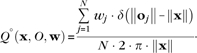(4)

Q°(x, O, w) is an estimator for the radial density of labeled locations O at a distance $\Vert \mathbf{x}\Vert$ from the injection site (taken to be the origin), normalized by the circumference of the circle passing through x. Each labeled location o_j has a weight w_j as in Equation (1). δ(x) is the Dirac delta function. The estimator Q°(x, O, w) is evaluated over a restricted space R ⊂ ℝ², y_i ∈ R, to compute the vector q:q_i = Q°(y_i, O, w) which comprises a radially symmetric density estimate for the labeling pattern under evaluation. This estimate is subsequently filtered through the same kernel density estimator D_κ,Φ as used for the reconstruction itself (Eq. 3). The normalizing factors in Equation (3) ensure that $P_{\text{Φ}}^{°}(\mathbf{x},\mathit{O},\mathbf{w},\mathit{R}\text{)}$ is a p.d.f. of the probability of observing a labeled cell at a point x in space, when evaluated over the space R. To determine a P value for each point x in space and locate significant clusters of label, we perform a Monte Carlo simulation of the radially symmetric model $P_{\text{Φ}}^{°}(\mathbf{x},\mathit{O}\text{)}$ (Eq. 3). A P value map and the significant cluster for the Gaussian mixture model example are shown in Figure S1c,d.

The only parameters under this analysis are the form and size of the kernel K used for estimating the density of labeled cells (Eq. 1). The kernel width effectively determines the spatial scale over which to look for regions of elevated density. Although a spatial scale close to that of the true cluster is probably optimal, the location and size of the identified clusters remain roughly constant over a wide range of kernel widths.

Model Framework and Generation of Axonal Arbors

A sheet of cortex is represented by a 2D plane, discretized into a fine square mesh with spacing δx (gray lines in Figure 3a,b,e—we take δx = 25 μm in this paper). Neuron and bouton locations u are constrained to fall on this mesh, that is, u ∈ ℝ², {p, q} ∈ ℕ, u = (p.δx, q.δx). Each mesh vertex contains a fixed number N of neuron somata. Neurons make axonal projections in straight lines (u, v) with uniform random directions across cortex (blue lines in Fig. 3a,c,d,f), with power law (scale free) distributed lengths and numbers of long-distance projections, and with maximum distance l (see Fig. 2).

Figure 3.

Connectivity rules used to generate axonal arbors. (a) Basic rule for projections unto a regular grid. Neuron somata exist on a square mesh (gray lines in a, b, and e); the neuron forming connections in this figure (black dot) can potentially project to the vertices of a triangular grid 𝒜_u (the patch grid—large gray circles in a, defined by H_ϑ,θ,_u), which has an origin that shifts with the location u of the neuron soma. A neuron makes clustered arborizations (blue dots in a, c, and f) when its axonal projection (blue lines) pass within a distance δa of the vertices of the patch grid. Neurons also make local isotropic connections with the region surrounding their soma (green dashed circles in a, c, and f). (b–d) Inhomogeneous connectivity models. A fixed regular grid is laid across the simulation mesh (magenta circles in b–f), defining regions of altered connectivity rules (Eq. 7). As illustrated in (c), most areas of cortex have a projection rule very similar to that in (a). Clustered arborizations (blue dots) are made for three reasons, indicated by the color of the circle surrounding each cluster: a local arborization surrounds each soma (dashed green circle); when an axonal collateral intersects with the shifting patch grid (black circles); and when a collateral intersects with the fixed, nonpatchy region grid (magenta circles) close to the neuron soma. Neuron somata that falls inside a region of altered connectivity (d) form a nonpatchy local arborization within a radius of 1.5 mm surrounding the soma (green shaded region in d, not shown to scale). (e) Another grid defining a third connectivity rule is included (green circles in e). (f) Neuron somata that fall inside this grid make clustered axonal projections as in (a–d), but with a larger maximum axonal spread.

Figure 2.

Distributions of the number (a) and length (b) of axonal collaterals arising from a single neuron. Both curves follow a power-law distribution.

Potential locations for clustered axonal arborizations are determined by the vertices of another grid, subject to the definition of connectivity rules in the model. For most of the models presented here the potential arborization locations 𝒜_u for a neuron are defined relative to the location u of the soma of that neuron and are determined by a connectivity function

(5)

where a single arborization location a_i,u ∈ 𝒜_u, a_i,u ∈ ℝ². The connectivity function C(u, Φ) defines the set of arborization locations arising from neurons at a location u in space and is parameterized by the set of parameters Φ. When an axon collateral passes within a threshold distance δa of an arborization region, it is considered to form a clustered arborization there. An isotropic Gaussian field of a fixed standard deviation σ_patch in width is placed at the corresponding vertex a_i of the arborization grid, that is,

(6)

Here the function 𝒢 determines the probability of observing a bouton at a location b near to the arborization location a_i, and ‖b, a_i‖ is the Euclidean distance between locations b and a_i on the simulated sheet. A fixed number B of synaptic boutons are placed randomly within the patch a_i, using function 𝒢 as a p.d.f. over which to draw the bouton locations. The number of boutons B generated by each terminal arborization was kept low for simulation efficiency. Changing this parameter did not affect the patterns of label produced by the models described here. We also use function G to define the local projection field of each neuron, with a standard deviation of σ_local. The set B_u,_n: b_i ∈ ℝ² is defined to contain the bouton locations for neuron n at location u in space.

The parameters for all models described in this paper are listed in Tables 1–5.

Table 1.

Model I: Parameters used for the homogenous, crystalline model (Figure 4)

δx	Discretization mesh spacing for bouton and somata locations: 25 μm
N	Number of neurons at each location u: 4
	Number of axonal collaterals per neuron: scale-free distribution, maximum 7 (see Fig. 2a)
l〈0〉	Axonal collateral length: scale free distribution, maximum 5440 μm
${\text{𝒜}}_{\mathbf{u}}^{\langle 0\rangle }$	Patch arborization locations for a neuron at location u: a shifting hexagonal lattice Hϑ,θ,u with origin u
ϑ〈0〉	Inter-patch spacing defined by the shifting hexagonal lattice: 680 μm
θ〈0〉	Lattice rotation: fixed at 0 degrees.
4.σpatch	Patch width: set to half patch spacing, that is, 4.σpatch = 340 μm
δa	Patch arborization distance threshold: 180 μm
4.σlocal	Local arbor width: equal to patch width, that is, 4.σlocal = 340 μm
B〈0〉	Number of boutons drawn per patch or local arborization per axonal terminal arborization: 5

Note: The process used to generate this model is illustrated in Fig. 3.

Table 5.

Model V: Parameters used for the model with nonpatchy regions as well as regions of longer patchy axonal spread (Fig. 7c,d)

l〈0〉	Default axonal collateral length: scale-free distribution, maximum 4080 μm
S〈2〉.	Seed “CO blob” locations for connectivity rule 2: a static hexagonal lattice $H_{\vartheta ,\theta ,\mathbf{\text{v}}}^{\langle 2\rangle }$ with origin at v〈2〉
δr〈2〉	Membership threshold distance for connectivity rule 2: 180 μm
v〈2〉	Origin for “CO blob” location lattice: interleaved with the nonpatchy region lattice: $(-{\vartheta }^{\langle 1\rangle }.\cos \left(\pi /6\right),0)$
ϑ〈2〉	Spacing defined for the static hexagonal lattice of “CO blob” locations: 680 μm
θ〈2〉	Lattice rotation: fixed at 0 degree.
l〈2〉	Axonal collateral length for “CO blob” locations: scale-free distribution, maximum 5440 μm
𝒜〈2〉	Patch arborization locations for a neuron at location u: a shifting hexagonal lattice $H_{\vartheta ,\theta ,\mathbf{\text{u}}}^{\langle 2\rangle }$ with origin u, as well as the pinwheel locations from S〈1〉 within a threshold distance dl.
B〈2〉	Number of boutons formed per axonal collateral by an arborization into a “CO blob” region: 5, that is, equal to B〈0〉

Note: Parameters not listed here are identical to those in Tables 1 and 4. The process used to generating this model is illustrated in Fig. 3.

Connectivity Patterns

The connectivity patterns we describe in this paper are based on regular triangular grids (gray circles in Fig. 3a). We use these grids to either define static absolute locations across a cortical sheet or to define positions relative to the location of a neuron soma. In the latter case, the grid shifts smoothly across our simulated cortex, following the locus of the soma for which it defines a connectivity rule. A triangular grid is appealing as it implies the most efficient use of cortical space—the tightest packing of putative equal-sized cortical units (Fejes Tóth 1940). However, the precise form of the periodic grid used to define connectivity does not affect the presence or absence of clustered labeling resulting from simulated injections.

The set of locations H_ϑ,θ,_u defines points h_i ∈ ℝ² falling on a triangular grid with vertex spacing ϑ, fixed rotation θ, and origin u with respect to the square discretization mesh. For static grids, u is a fixed location within the simulated cortical sheet. For smoothly shifting grids, u is taken to be the location of the neuron soma that is using the grid to form connections. In the work described here, we often use H_ϑ,θ,u as a connectivity function in the sense of Equation (5).

Some models we define have more than a single connectivity rule. For these models, we use the notation ConnectivityRule(u,m) to indicate that neurons at location u fall under connectivity rule set m, m ∈ [1 … M]. A neuron at a location u in space meets this criteria when u is closer than a threshold distance δr^〈m〉 from a point ${\mathbf{\text{s}}}_i^{\langle m\rangle }$ in a set of seed locations S^〈m〉 (small circles in Fig. 3b–f); that is,

(7)

Seed locations S^〈m〉 are usually defined by hexagonal lattices, similar to those used to define patch locations. By default, unless overridden by Equation (7), every location falls under connectivity rule m = 0. Parameters for connectivity rule m are indicated by the superscript ^〈m〉, for example, ${\sigma }_{\mathit{patch}}^{\langle 0\rangle }$ defines the standard deviation of a patch field under the default connectivity rule.

Simulated Injections and Transport

We simulate injections of neural tracer into our sheet of cortex using a simple model of non–trans-neuronal transport. To bypass the uncertainty of precisely where tracer is absorbed for a given injection size and injection method, we directly define a tracer uptake zone on our simulated cortical sheet, consisting of a set T : t_i ∈ ℝ² of labeled locations. Somata and boutons within this area are considered to have absorbed an equal amount of neural tracer, sufficient to label the entire cell through anterograde and retrograde transport.

Transport is determined by the spatial arrangement of a simulated population of neurons and their axonal arbors and boutons, without regard to activity or function. Retrograde transport occurs only between the tracer uptake zone T and neurons across the sheet that form boutons within the uptake zone; that is, a neuron n at location u will receive retrograde label under the condition

(8)

Neurons whose somata fall within the tracer uptake zone are considered to be retrogradely labeled, under the condition

(9)

Anterograde transport occurs between labeled somata and the boutons that form the axonal arborization of those somata. This is described by the condition

(10)

Note that the combination of Equation (8) and Equation (10) implies that retrogradely labeled somata will have their own axonal projection labeled through bidirectional tracer transport.

Detailed Model Descriptions

Model I—Shifting Patch Grids

The connection pattern that underlies all the models described here comprises projections onto a regular triangular grid (Fig. 3a). In our simplest model, the origin of this projection grid shifts with the soma of the neuron making an axonal arbor (black dot in Fig. 3a). Parameters for this model are given in Table 1.

To generate connectivity in Model I, we place a hexagonal grid H_ϑ,θ,u across the cortical surface for each pyramidal cell soma (gray circles in Fig. 3a) with the grid origin at the location u of that soma (black dot in Fig. 3a), with a intervertex spacing of ϑ = 680 μm and with a fixed orientation θ. This grid defines the potential arborization locations 𝒜_u for that cell. The width of arborization zones (defined as 4.σ_patch; see Equation 6) is set at half the patch spacing (340 μm). Axons formed a clustered terminal arborization into a patch location when passing within δa = 180 μm of a patch location a_i,_u.

The arrangement of projections from a single cell in this model is illustrated in Figure 3a. In addition to an isotropic local arborization, a neuron at a given point in our simulated cortex arborized preferentially on to a hexagonal grid of a fixed spacing, with its origin at the location of the neuron's soma (the “patch grid” H_ϑ,θ,u). The vertices of this grid, 𝒜_u, are used as the peaks of the Gaussian fields that defined arborization probability, as described above (Eqs 5 and 6). The patch grid H_ϑ,θ,u, carrying with it the potential arborization locations for a given cell, shifts smoothly across the surface of our simulated cortical sheet. Despite the underlying regularity and homogeneity of the connectivity rules for each neuron, axonal arbors made by single neurons are highly anisotropic and highly individual (Fig. 3a).

Model II—Static Patch Grids

This model introduces the concept of a static patch grid, predefined for the cortical sheet through some mechanism outside the model. The patch grid has the same form as illustrated in Figure 3a, but with a fixed origin. Every neuron in Model II makes “convergent” axonal projections onto those predefined patch locations. Formally, we define a set of global patch locations 𝒜^〈0〉 as the hexagonal lattice of points H_ϑ,θ,0, with an inter-vertex spacing of ϑ = 680 μm, rotation θ = 0 degrees and origin at (0, 0) (see Table 2 for the full list of parameters). In contrast to Model I, the set of possible arborization locations 𝒜_u no longer depends on the location of a source neuron, and so is identical for each neuron ($\forall \mathbf{\text{u}}:{\text{𝒜}}_{\mathbf{\text{u}}}^{\langle \mathrm{0}\rangle }={\text{𝒜}}^{\langle 0\rangle }$). In addition to isotropic local arbors, neurons generate clustered terminal arbors when an axonal collateral passes near to a global patch location. This model produces a network in which every neuron participated in the static, global patch system, and where axonal projections converged globally onto the discrete patch locations defined by 𝒜^〈0〉.

Table 2.

Model II: parameters used for the globally convergent model (Fig. 5a–c)

${\text{𝒜}}_{\mathbf{\text{u}}}^{\langle 0\rangle }$

Patch arborization locations for a neuron at location u: defined globally for all neurons by the set ${\text{𝒜}}_{\mathbf{\text{u}}}^{\langle 0\rangle }=H_{\vartheta ,\theta ,\mathbf{\text{0}}}^{\langle 0\rangle }$: a static hexagonal lattice $H_{\vartheta ,\theta ,\mathbf{\text{0}}}^{\langle 0\rangle }$ with origin at (0, 0)

Note: Parameters not listed are identical to those in Table 1. The process used to generate this model is illustrated in Fig. 3.

Model III—Regions of Altered Connectivity

This model further restricts which regions across the cortical sheet participate in the patch system. As for Model II, discrete patch locations are globally defined at the vertices of a hexagonal lattice (i.e., $S^{\langle 1\rangle }=H_{\vartheta ,\theta ,\mathbf{\text{0}}}^{\langle 1\rangle }$—see Table 3 for a full list of parameters). However, Model III uses an alternative connectivity scheme for neurons falling close to the set of globally defined patch locations (see Eq. 7). Neurons falling within a threshold distance (δr^〈1〉 = 180 μm) of a patch location make long-range, clustered terminal arborizations onto the previously defined patch locations $H_{\vartheta ,\theta ,\mathbf{\text{0}}}^{\langle 1\rangle }$. All other neurons make only local, nonpatchy arborizations (i.e., ${\text{𝒜}}_{\text{u}}^{\langle 0\rangle }=\varnothing$). This model relaxes assumption 8, meaning that many locations across the cortical sheet do not participate in the patch system.

Table 3.

Model III: parameters used for the discrete patch location model (Fig. 5d–f)

${\text{𝒜}}_{\mathbf{\text{u}}}^{\langle 0\rangle }$	Default patch arborization rule: ${\text{𝒜}}_{\mathbf{\text{u}}}^{\langle 0\rangle }=\varnothing$, that is, nonpatchy projections
S〈1〉	Seed locations for connectivity rule 1: a static hexagonal lattice $H_{\vartheta ,\theta ,\mathbf{\text{0}}}^{\langle 0\rangle }$with origin at (0, 0)
δr〈1〉	Membership threshold distance for connectivity rule 1: 180 μm
ϑ〈1〉	Spacing defined for the static hexagonal lattice: 680 μm
θ〈1〉	Lattice rotation: fixed at 0 degree.
${\text{𝒜}}_{\mathbf{\text{u}}}^{\langle 1\rangle }$	Patch arborization locations for a neuron at location u under connectivity rule 1: globally defined patch locations under the set ${\text{𝒜}}_{\mathbf{\text{u}}}^{\langle 0\rangle }=H_{\vartheta ,\theta ,\mathbf{\text{0}}}^{\langle 1\rangle }$, that is, the same locations as S〈1〉.

Note: Parameters not listed are identical to those in Table 1. The process used to generate this model is illustrated in Fig. 3.

Model IV—Orientation Pinwheel Zones

This model introduces the assumption of fixed zones, based on observations of orientation pinwheels in primary visual cortex, that only partially participate in the patch system (assumption 9—Yousef et al. 2001). The process for defining connectivity in this model is illustrated in Figure 3; the full list of parameters for this model is given in Table 4. The basic connectivity rule is that of Model I—neurons project to patch locations on a hexagonal grid H_ϑ,θ,u, with the origin at the location u of the neuron soma (Fig. 3a). In addition to this shifting patch grid, we place a fixed hexagonal grid across our cortical sheet, the vertices of which correspond to regions of modified connectivity (nonpatchy regions) which are designed to have an isotropic connectivity pattern similar to that observed at pinwheel centers (Fig. 3b). Neurons within a threshold distance δa = 180 μm of these points do not participate in the patch system and make only local isotropic projections (Fig. 3d). In addition, all neurons across the cortical sheet project to nonpatchy regions that fall close to their soma (Fig. 3c).

Table 4.

Model IV: parameters used for the model with nonpatchy regions (Figs 6 and 7a,b)

S〈1〉	Seed nonpatch area locations for connectivity rule 1: a static hexagonal lattice $H_{\vartheta ,\theta ,\mathbf{\text{0}}}^{\langle 1\rangle }$ with origin at (0, 0)
δr〈1〉	Membership threshold distance for connectivity rule 1: 180 μm
ϑ〈1〉	Spacing defined for the static hexagonal lattice of “pinwheel” locations: 680 μm
θ〈1〉	Lattice rotation: fixed at 0 degree.
${\text{𝒜}}_{\mathbf{\text{u}}}^{\langle 1\rangle }$	Patch arborization rule 1 for “pinwheels”: ${\text{𝒜}}_{\mathbf{\text{u}}}^{\langle 1\rangle }=\varnothing$, that is, only local, nonpatchy, projections
B〈1〉	Number of boutons formed per axonal collateral by an arborization into a nonpatch area: 2
${\text{𝒜}}_{\mathbf{\text{u}}}^{\langle 0\rangle }$	Patch arborization locations for a neuron at location u: a shifting hexagonal lattice $H_{\vartheta ,\theta ,\mathbf{\text{0}}}^{\langle 0\rangle }$with origin u, as well as the “pinwheel” locations from S〈1〉 within a threshold distance d1.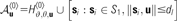
dl	Distance over which patch-projecting neurons arborize into “pinwheel” locations: 1.4 × ϑ〈0〉 = 952 μm

Note: Parameters not listed here are identical to those in Table 1. The process used to generate this model is illustrated in Fig. 3.

Model V—CO Domains

This model introduces the final rule for generating connectivity, based on observations of CO blobs in primary visual cortex (assumption 10—Livingstone and Hubel 1984a). As in Models I and IV, most neurons make clustered arborizations onto the vertices of a shifting hexagonal grid $H_{\vartheta ,\theta ,\mathbf{\text{u}}}^{\langle 2\rangle }$ with the origin at the location u of the neuron soma (Fig. 3a). However, the maximum axonal projection distance under the default connectivity rule, l^〈2〉, is reduced to a scale-free distribution spanning 4080 μm (the full list of parameters for Model V is given in Table 5). Similarly to Model IV, we introduce static, predefined regions $H_{\vartheta ,\theta ,\mathbf{\text{0}}}^{\langle 1\rangle }$ following a hexagonal lattice, within which neurons make only local, nonpatchy projections (Fig. 3b,d). In addition, we introduce another set of static, predefined regions, also based on a hexagonal lattice, representing regions of high coreactivity as described above (assumption 10—Fig. 3e,f). Neurons within a threshold distance (δr^〈2〉 = 180 μm) of these points make clustered axonal arborizations over a longer distance (l^〈2〉 = 5440 μm) than neurons falling elsewhere on the simulated cortical surface (Fig. 3f). The hexagonal lattice $H_{\vartheta ,\theta ,\mathbf{\text{v}}}^{\langle 1\rangle }$ that defines these simulated CO blob regions is interleaved with the lattice $H_{\vartheta ,\theta ,\mathbf{\text{v}}}^{\langle 1\rangle }$ defining the nonpatchy regions, by setting the mesh origin $\text{v}=(-{\vartheta }^{\langle 1\rangle }.\cos (\pi /6),0)$, where ϑ^〈1〉 is the lattice spacing, ϑ^〈1〉 = 680 μm (Fig. 3e). Note that the rotations θ^〈*^〉 of the hexagonal meshes are aligned, that is θ^〈0〉 = θ^〈1〉 = θ^〈2〉. The alignment or otherwise between these meshes does not greatly impact the qualitative dynamics of simulated labeling in this model, but see our discussion below.

Results

Model I: A Simple, Smoothly Shifting Patch System

The frequent experimental observation of a semi-regular system of patches, centered on the site of a small injection of tracer, lead us to propose an intuitive model of projections onto a regular grid (assumption 2) that shifts smoothly across the cortical surface. This model carries the implicit assumptions that for two small, offset injections of tracer, the locations of clusters of label for the two resulting patch spreads will have a consistent geometric relationship (assumption 3) and that any small injection will result in a clustered pattern of label (assumption 8). Shifting the location of an injection site causes an identical shift in the locations of the revealed patches. This model made the minimal assumptions for the rules used to construct the patch system: that the architecture of the projections underlying the patch system is identical for each neuron and requires only information available internally to that neuron.

Figure 4a,b show the pattern of label resulting from a small (160 μm diameter uptake zone) simulated injection of an anterograde tracer into this model. Only a small number of neurons were labeled, and the anisotropic nature of the individual neural arbors was reflected in the anisotropic pattern of labeling in Figure 4a,b. The complete, grid-like pattern of projections made by the small population of labeled neurons is more clearly visible when simulated injections of bidirectional tracers are used Figure 4c,d (Eqs 8–10).

Figure 4.

Model I: The distribution of label following simulated injections of anterograde and bidirectional tracers into a homogenous crystalline model. White circles: Injection uptake zone. Gray scale values: density of labeled boutons. Black dots in (a) and (c): retrogradely labeled somata. (a, c, e, and g) Patterns of labeling following simulated injections of anterograde (a) and bidirectional (c, e, and g) tracers. (b, d, f, and g) Significant clusters of label (P < 0.01), as determined by our patch-seeking density analysis method applied to bouton labeling only; conventions as for Figure S1d,h,l. Injection diameters: a–b 160 μm; c–d 160 μm; e–f 600 μm; g–h 2000 μm. Scale bars: 1 mm.

Due to the crystalline nature of the underlying connections between points across the simulated cortical sheet under Model I, the pattern of label formed by a simulated injection was roughly predicted by convolving the injection site with the patch grid. As a result, the diameter of labeled clusters of boutons was directly determined by the diameter of the injection site. This can be seen in Figure 4e,f, which show the pattern of label following a larger (600 μm diameter uptake zone) simulated injection of a bidirectional tracer. The remote clusters of label were roughly the same size as the new injection site and considerably larger than in Figure 4c,d. This effect was exacerbated by very large injections as can be seen in Figure 4g,h. As expected from a convolution between the crystalline lattice and an injection site larger than the nominal lattice spacing, the degree of segregation of individual patches was reduced and finally disappears completely. This is in stark contrast to the structured labeling patterns that result from large injections in vivo, as discussed above (observations A and B).

Model II: Globally Defined Patch Locations

Following the failure of a purely locally defined architecture to reproduce the labeling patterns observed in cortex, we investigated the implications of a purely global definition of patch locations (abandoning assumption 3). Our first such model assumed that the locations of patches were predefined across cortex through some mechanism outside the model and that every neuron made convergent axonal projections onto those predefined patch locations. This model produced a network in which every neuron participated in a static, global patch system and where axonal projections converged globally onto discrete patch locations.

Figure 5a,c show the predicted labeling patterns resulting from simulated injections into this model. Small injections of anterograde and bidirectional tracers made into any location across the simulated cortical sheet produced a clustered pattern of labeled boutons radiating from the injection site (Fig. 5a,b). By definition, these patches of anterograde label fell at the locations of the patch arborization lattice and were fixed in diameter. However, retrograde labeling of somata was diffuse (Fig. 5b,c), in contrast to the colocated clusters of anterograde and retrograde labeling frequently reported in the literature (observation C— e.g., Rockland et al. 1982; Tyler et al. 1998; Angelucci et al. 2002b). When a small injection was made outside a predefined patch area, a small field of somata surrounding the injection site was labeled through retrograde filling of local axonal arborizations (Fig. 5a). Small injections into global patch areas resulted in diffuse labeling of somata across the simulated cortical sheet, reflecting the widespread convergence of projections into these locations (Fig. 5b).

Figure 5.

Models II and III: Models of the patch system based on the definition of global patch locations. Magenta dots: retrogradely labeled somata. Other conventions as in Figure 4. (a–c) Simulated injections of bidirectional tracers into Model II. (a) 200 μm diameter injection outside static patch zone; (b) 200 μm, injection inside static patch zone; (c) 2000 μm injection spanning static patch and nonpatch zones. (d–f) Simulated injections of bidirectional tracers into Model III; (d) 200 μm, injection outside static patch zone; (e) 200 μm, injection inside static patch zone; (f) 2000 μm injection spanning static patch and nonpatch zones. Scale bars: 1 mm.

Model II was defined by globally convergent projections onto a set of discrete patch locations, and thus, the anterograde transport of tracers also converges globally onto these locations. A corollary of this convergence of projections is that retrograde transport “diverges” from any point across the cortical sheet, leading to diffuse labeling of somata. The inverse model, in which discrete, predefined patch locations project widely across cortex while all other areas project only locally, would exhibit the reverse pattern of labeling. Small injections would result in clusters of labeled somata but diffuse anterograde labeling of boutons. Neither model formulation reflects the qualitative dynamics of patch system labeling in cortex, fundamentally due to the coupling displayed between divergent and convergent tracer transport, in opposite transport directions.

Model III: Discrete Regions of Patchy Projection

We removed the coupling between divergent and convergent transport in a third model of axon formation. As for Model II, discrete patch locations were globally defined. However, in Model III, only neurons falling within globally defined patch locations made clustered axonal projections to other patches. All other neurons did not participate in the patch system and made only local, nonpatchy arborizations.

The patterns of label predicted by simulated injections of neural tracers into this model are shown in Figure 5d–f. Small injections into a patch zone produced colocated clusters of labeled boutons and somata spreading across the surface of cortex (Fig. 5d), as did large injections covering several patch zones (Fig. 5f). However, small injections outside a patch zone resulted only in local, diffuse labeling (Fig. 5e). Since the majority of the simulated cortical sheet fell outside patch zones, most small injections did not produce patches of label under this model. This prediction directly conflicts with the assumption that most small injections in vivo do indeed reveal the patch system, as discussed above (assumption 8).

Models II and III produced clusters of label in predefined locations across the cortical sheet, irrespective of the location of each injection. Researchers commonly assume that adjacent injections into a single cortical area in vivo would result in distinct sets of patches with a topographic relationship; a smooth shifting of patch locations with the locus of an injection site (assumption 3—Lund et al. 2003). Since global patch location models violate this assumption, we returned to models that are consistent with a smoothly shifting patch system.

Model IV: Inhomogeneous Connectivity Rules and Shifting Patches

As mentioned above, orientation pinwheel centers in primary visual cortex do not participate in the patch system but instead make and receive isotropic, functionally nonspecific projections with the local surrounding cortex (Sharma et al. 1995; Yousef et al. 2001; Mariño et al. 2005). We incorporated this observation into a model by introducing static, globally defined regions that made and received only local projections.

The patterns of labeling produced by small injections predicted by this model are shown in Figure 6a–f. As expected, simulated injections of both anterograde and retrograde tracers into nonpatchy regions produced diffuse labeling surrounding the injection site (Fig. 6a,b). Small injections into all other regions across the cortical surface produced colocated clusters of labeled boutons and somata (Fig. 6c,d—arrowheads indicate corresponding clusters).

Figure 6.

Model IV: Simulated injections of anterograde (a, c, e—labeled boutons) and retrograde (b, d, f—labeled somata) tracers into a model with regions of nonpatchy connectivity. Conventions as in Figure 4; (a and b) 200-μm diameter injections into nonpatchy regions; (c and d) 200-μm injections outside nonpatchy regions; (e and f) 800-μm injections spanning patchy and nonpatchy regions. Injections (c) and (d) are aligned; arrowheads indicate corresponding locations in (c) and (d). Labeled somata in (f) fall inside the labeled regions in (e) and not in the lacunae. Scale bars: 1 mm.

Larger simulated injections showed a complex pattern of labeling (Fig. 6e,f). Outside a dense region of label close to the injection site corresponding to labeling of local axonal arbors, the pattern broke up into regions of sparse labeling (lacunae, following the nomenclature of Rockland and Lund [1983]) surrounded by a lattice of densely labeled boutons and somata (satisfying observation B). Retrogradely labeled somata fell inside the lattice walls and usually not inside lacunae (observation C). Since the majority of areas across our simulated cortical sheet formed projections using the shifting patch grid, the underlying dynamics of large injections and small injections into patchy projection areas were very similar to that of Model I. In particular, labeling patterns under this model were still roughly predicted by convolving the injection site with the structure of the shifting patch grid. The regions of nonpatchy connectivity falling within an injection site circumscribe areas that do not participate in this convolution, leaving lacunae across the simulated cortical surface. Due to these convolution dynamics of labeling, Model IV does not limit patches to a maximum size, and so very large injections result in diffuse labeling similar to that shown by Model I (cf. Fig. 4g,h).

A very large simulated injection of bidirectional tracer into this model is shown in Figure 7a–c, using the same cortical sheet as in Figure 6. The lacunae structure was still evident, especially in the pattern of labeled somata (Fig. 7a), and highlighted by the low P values (green areas in Fig. 7b) indicating significantly reduced labeling. However, the degree of clustering distant from the injection site was minimal, evidenced by the lack of statistically significant labeling in Figure 7c. One more element is required to fully reproduce every aspect of the clustered labeling patterns seen in cortex: a rule is needed that produces discrete clusters of label far from a large injection site.

Figure 7.

Models IV and V: Very large simulated injections into a model with nonpatchy regions (Model IV: a–c) and an model with regions of longer projections (Model V: d–f). Conventions as in Figure 5. (a and d) Simulated injections of bidirectional tracers. (b and e) P value maps indicating regions of anisotropic labeling. Green regions indicate weaker labeling than expected; red regions indicate stronger labeling than expected; color intensity indicates the estimated P value of the observed deviation from isotropic labeling. (c and f) Regions of significantly elevated labeling density (P < 0.01). Scale bars: 1 mm.

Model V: Regions of Longer Projections

The observation by Livingstone and Hubel (1984b) that most distant labeled patches are colocated with CO blobs in visual cortex implies that neurons in CO-rich domains make longer horizontal axonal projections than neurons elsewhere across cortex. We accordingly introduced a fifth and final model reflecting this phenomenon, in which neurons whose somata fell inside small, predefined regions had larger axonal fields than elsewhere across the simulated sheet (assumption 10).

Small injections into this final model appeared qualitatively identical to those for Model IV, as in Figure 6a–d. The exception is when small injections were made into simulated CO regions, in which case labeled patches spanned a larger distance across the cortical surface. A very large injection into Model V is shown in Figure 7d–f, for comparison with a similar large injection into Model IV (cf. Fig. 7a–c). The P value map again highlights significant lacunae (green areas in Fig. 7e), but in contrast to Model IV significant clusters of label formed far from the injection site (Fig. 7f, satisfying observation A). These distant discrete clusters fell inside simulated CO blobs.

Discussion

We defined a simple model for connectivity across a simulated cortical sheet, where each point in cortex projects preferentially on to the vertices of a regular triangular grid surrounding that point (Model I). “Crystalline” models such as this are attractive since they explain the regular clusters of label resulting from most small injections of tracer and echo the regularity in functional maps that exists in primary visual cortex of higher mammals. Models with this fundamental structure follow directly from the assumption of projections between regions of similar function (like-to-like projections), over a periodic functional map. However, these models fail due to their prediction of diffuse labeling for large injections, contrary to the punctate labeled patterns observed in vivo (observation A—see Fig. 4g,h). The reason for this failure is fundamentally due to the use of a homogeneous rule for connectivity across cortex. This failure will affect any “like-connects-to-like” functional model that uses a single connectivity rule over a periodic functional map.

We proposed a model that qualitatively reproduced all aspects of cortical labeling patterns by breaking the homogeneity of our connectivity rules (Model V). We defined a system where some small areas of cortex used different rules for connectivity, justified by the observation of altered labeling patterns when small injections are made into the centers of orientation pinwheels in visual cortex (assumption 9—Yousef et al. 2001) and by the observation that labeled patches distant from a large injection fall over CO blobs in primate visual cortex (assumption 10—Livingstone and Hubel 1984a). This model displayed complex patterns of labeling following simulated injections of tracer. Small injections into most areas of cortex resulted in clusters of colocated anterograde and retrograde label spreading from the injection site, with short bands or extended bars close to the injection site (observation C). Small injections made into zones of isotropic connectivity produced local, diffuse patterns of anterograde and retrograde labeling (following from assumption 9, and as observed for injections in cortex—Yousef et al. 2001). Large simulated injections lead to a complicated pattern of label including areas close to the injection site with reduced staining, separated by bands of intense label. Areas of reduced labeling fell over isotropic connectivity zones and are qualitatively similar to the lacunae observed near large injections in vivo (observation B—Rockland and Lund 1983). Further from our simulated injection site, the bands of label separated into a pattern of discrete clusters, similar to the patterns observed following large injections into cortex (observation A—Rockland et al. 1982; Rockland and Lund 1983; Tyler et al. 1998).

The success of this model raises two key predictions for the patch system in visual cortex. The first is the existence of neurons within CO blobs that make long-range, clustered projections over longer distances than do patch-projecting neurons outside CO regions. While the presence of these neurons was earlier predicted by Livingstone and Hubel (1984a), no direct comparative study has been performed that would demonstrate their existence. Yabuta and Callaway (1998) reconstructed the axonal arbors of intracellularly filled neurons from tangential slices of macaque monkey primary visual cortex, collated by the CO compartment containing the reconstructed soma. While they did not report lengths and extent of axonal arbors, the number of patches formed by neurons within CO blobs did not differ significantly from the number of patches formed by neurons in inter-blob regions. Since these cells were filled in slices of cortical tissue and not in vivo the longest axonal projections would likely be cut, biasing this measure toward shorter projections. Their study cannot therefore be considered definitive, leaving this question unanswered.

The second prediction raised by our model relates to the zones of nonpatchy connectivity, which correspond to orientation pinwheels in primary visual cortex (Yousef et al. 2001). Since these zones correlate with a marked modification of the structure of the patch system, orientation pinwheels may not be merely a consequence of mapping several functional modalities onto an overlapping representational space, as suggested by Swindale et al. (2000). In particular, pinwheels may determine the locations of the lacunae seen in visual cortex following very large injections of tracer. Large injections into primary visual cortex in vivo, aligned with functional maps of orientation preference, should show that orientation pinwheel zones correspond to unlabeled lacunae.

Lattice-like labeling patterns with lacunae also exist in other, nonvisual areas of cortex (e.g., monkey prefrontal cortex—Levitt et al. 1993). If the patch system in these areas also turns out to smoothly shift across the cortical surface, then unlabeled lacunae should correspond to regions of unclustered connectivity similar to pinwheel zones. In this case, pinwheel-like regions may be essential to the general structure of the patch system, rather than a consequence of functional encoding in primary visual areas. Nascent structural correlates of future pinwheel zones may exist as “seed points” during the development of the superficial patch system, with the intriguing implication that orientation pinwheels in v1 may in fact be a consequence of patch system formation.

Our Model V has a few potential shortcomings. First, the model is still fundamentally based on a homogenous, crystalline patch lattice. As described above, such homogenous systems predict labeling patterns where the diameter of patches has a direct linear relationship with the size of an injection uptake zone. Labeling patterns in cortex certainly show a maximum patch size (observation A), but it is unclear whether smaller labeled patches are revealed by smaller injections. Such a relationship has been reported (Lund et al. 1993), although has not been rigorously quantified.

Second, the model assumed that regions of nonpatchy projections (simulated pinwheel zones) are interleaved with simulated CO regions. This assumption is justified by the experimental observation that CO regions always fall within the labeled walls surrounding lacunae (Rockland and Lund 1983). However, their precise interleaved alignment is not essential to the model. Allowing the two systems to move out of phase by relaxing the requirement that they should interleave causes a conflict between the two connectivity rules only where regions defined as static patches overlap with regions defined as nonpatchy. Where such an overlap occurs, connectivity is undefined and must either result in single lacunae that are labeled or lead to holes in the labeled lattice surrounding a large injection. The degree of phase slip between the two systems determines how frequently this overlap occurs.

Finally, in simulating the uptake of neural tracer, we assumed a flat distribution of tracer throughout an uptake zone, ignoring the effects of diffusion, which might vary considerably between implanted crystal tracers such as DiI and liquid tracers such as hrp. Aside from investigating the effects, a diffusing tracer might have on the labeling patterns predicted in this paper, assuming a Gaussian field for the injection site might itself increase the appearance of clustering in several of the models discussed in this paper.

Patchy Labeling across Cortex

Cortical areas in the early and intermediate visual hierarchy contain a relatively regular and periodic patch system (e.g., V1, V2 and MT—assumption 2). Labeling patterns following injections into visual areas are difficult to reproduce due to the combination of this regular periodicity with the assumption of a smoothly shifting patch system (assumption 3). Although we attempted to design models applicable to any cortical area, in order to explain the hard problem of patchy labeling in visual cortex following large injections, we were forced to incorporate several structural properties of area V1. As discussed above, their inclusion predicts the presence of similar structural correlates in other cortical areas that display similar complex labeling patterns. However, the inclusion of these anatomical features of cortex implies no assumption of their function for cortex, meaning that our models are nevertheless agnostic to cortical function.

Nonprimary visual areas (e.g., IT cortex and frontal areas) show far less regularity in the arrangement of patches and in the arrangement of cortical responses. Removing the assumption of a regular periodic patch system would be justified if small populations of neurons, on the scale of single patches or single functional domains in cortex, collectively made projections to a common set of patches arranged across cortex in an unpatterned manner. The functional arrangement in area IT, which represents complex objects by the conjunctive activity of several cortical domains arranged aperiodically across cortex (Wang et al. 1996), might require such a patch system. Relaxation of the periodicity assumption (assumption 2) breaks the “spatial convolution” behavior of patch system labeling. Reproducing punctate and lattice-like labeling patterns for very large injections then becomes trivial.

Alternatively, relaxing our assumption of a smoothly shifting patch system (assumption 3) and defining a single, static patch system across cortex results in our models II and III. That architecture would be justified if the functional arrangement in a cortical area was not continuous but contained static areas coding for different functions; for example, similar to the arrangement of ocular dominance columns (LeVay et al. 1975; Shatz et al. 1977) or color-coding regions in V1 (Livingstone and Hubel 1984a). Relaxing this assumption also breaks the convolution-like behavior of cortical labeling patterns, making it simple to limit the maximum labeled patch size for large injections.

Patchy Labeling in Rodents

While the presence of a patch system in primates and higher mammals is uncontroversial, some ink has been spilt arguing whether an equivalent system is present in the rodent. Bulk injections of bidirectional tracers into rodent visual cortex reveal undeniable axonal clusters (Burkhalter 1989; Kaas et al. 1989), but retrograde labeling produces only equivocal clustering at best (Burkhalter and Charles 1990; Van Hooser et al. 2006; see Fig. 1c,d). Although no neuronal substrate for a “horizontal,” intralaminar patch system has been demonstrated in rodent cortex, neurons in lower layer 5 and in layer 6 send a distinctly clustered and periodic projection to layers 2–4 (Burkhalter 1989). This combination of clustered anterograde and unclustered retrograde labeling can be explained by our Model II. In this model, neurons everywhere across a cortical area make clustered axonal projections to a static, predefined set of patch locations.

Further confirmation of this putative projection scheme could be had by examining whether patch locations in rodent cortex are truly static or whether they shift with the location of an injection site. Multiple offset injections of distinguishable anterograde tracers would directly address this question. Experimental validation could also be obtained by measuring the spacing between a small injection site and the nearest patches—the geometry of a static patch system implies that most injections will not fall directly over a patch or equidistant between patches, and so the injection site is likely to be disproportionately close to one labeled patch over others. In contrast, labeling a smoothly shifting patch system such as that of Model I will always result in an injection site equidistant from the nearest labeled patches. Although this prediction offers a route to differentiate between Models I and II, it may prove difficult to distinguish a labeled patch close to the injection site from the local axonal arbors of labeled cells.

Conflict between Convergent and Divergent Connectivity

The observation of discrete patches of label after large injections of tracer leads one to conclude that some amount of convergence must exist between the clustered axonal arbors of superficial layer pyramidal cells. Accordingly, we defined a model incorporating hard convergence of projections onto predefined, static patch areas (Model II). However, global “convergence” in one direction of tracer transport directly implies global “divergence” of transport in the opposite direction, as revealed by simulated injections into our model (Fig. 5a–c). Both convergence and divergence of axonal projections lead to models with clustering of label in only a single transport direction, with diffuse labeling following transport in the opposite direction. How then can one reconcile the formation of discrete patches of label following large tracer injections with convergence of axonal projections?

This conundrum was solved by our final model (Model V). Zones of longer axonal projection effectively limited the transport from a large injection to discrete patch locations far from the injection site. The connectivity rule that defined the static patch locations also ensured that axonal projections made from those same locations were longer than the projections for any other connectivity rule. Consequently, at some distance from a simulated injection location, connectivity rule 2 dominated the projections to and from the injection site, to the exclusion of the connectivity rules that contributed to the pattern of label close to an injection. Far from an injection site, transport of tracer was therefore restricted to global, static patch locations.

Interpretation of Cortical Labeling Patterns

The interpretation of patterns of label resulting from injections of tracer in vivo is frequently complicated by bidirectional transport of tracer. The presence of retrogradely labeled neuron somata leads to uncertainty in the origin of any anterograde label. Labeled boutons and axonal segments may arise from neurons with somata at the injection site, from the local axonal arborization surrounding retrogradely labeled pyramidal cells, or from retrogradely labeled neurons situated away from the injection site which send an labeled axonal projection to a third point in cortex.

Consequently, labeled regions far from an injection site can be incorrectly identified as “axonal” patches, when they in fact consist only of one or more retrogradely labeled pyramidal cells and their labeled local arborization. The same issue can lead to incorrect identification of patchy structure in interareal projections: a large injection into a cortical area “area I” can label projection neurons in a second cortical area “area II” through retrograde transport. If those labeled neurons participate in a patch system intrinsic to area II, it may incorrectly appear as though area I sends a patchy feedforward projection to area II. A similar obfuscation occurs if the source of the area II → I projection is arranged in a periodic pattern across area II.

While most neural tracers are never purely anterograde or retrograde—especially under the experimental conditions of large pressure injections—we were able to restrict our simulated injections to a single transport direction, or to enable combined retrograde and anterograde transport. We found that for various simulated connectivity structures, bidirectional transport lead to significantly different patterns of label (Fig. S2). In light of this issue, we encourage researchers engaged in tracer injection experiments, as well as those interpreting the results of these experiments, to be circumspect in drawing their conclusions.

Implication of Pinwheel Injections

Although bulk injections of anterograde tracers reveal the unclustered distribution of axonal arbors arising from neurons at pinwheel centers (Sharma et al. 1995; Yousef et al. 2001; Mariño et al. 2005), the implications of nonclustered retrograde labeling from pinwheel injections is more subtle. Yousef et al. (2001) demonstrated that neurons close to a pinwheel collectively project to the pinwheel center; however, this does not imply that the axonal arbors of those neurons do not form clustered terminations elsewhere across the cortical surface. Simulated injections of an efficient bidirectional tracer into a pinwheel zone produced weak clusters of labeled boutons distant from the injection, even though the somata of the labeled neurons that provided the source of the clustered terminals were uniformly distributed around the injection site (Fig. S2). Weak experimental evidence for this can be seen in the results of Yousef et al. (2001—see their Fig. 2). Bidirectional labeling leading to the visibility of patches is likely to be overestimated by our model since our simulated tracers have equal efficacy for anterograde, retrograde, and bidirectional transport; a characteristic unlikely to be exhibited by chemical tracers. Although many neural tracers are not transported in a purely anterograde or retrograde manner, most tracers have a greater efficacy in one transport direction. We expect that large in vivo injections of bidirectional neural tracers into pinwheel centers could hide the uniform connectivity structure present there.

Our model of axonal projections from neurons near pinwheel centers assumed that the axonal arbors of single neurons were unclustered (see Fig. 3). Alternatively, individual neurons might make clustered axonal arbors but with no collective arrangement. Under this new assumption, labeling groups of neurons would still produce the diffuse labeling required for our models and observed in vivo.

Information Required for Patch System Development

We have shown that a model that assumes an identical distribution of connectivity for all neurons, constructed only with information available internally to each neuron, cannot reproduce the clustered labeling patterns seen in cortex. Neurons do not know where their somata lie in relation to other neurons across cortex and so in this model cannot cooperate to converge their clustered projections with those of other cells. In fact, the degree of rotational alignment between the axonal arbors of neurons inherent in our Model I is already difficult to justify from this perspective. This model is likely to be the best one can propose that relies only on neuron–local information, as any other arrangement of neural arbors will produce a lesser degree of clustered labeling.

Our Model V relies on information shared between neurons across the cortical sheet. In this particular model, the shared information was supplied without neural activity, by allowing all neurons knowledge of whether or not they fell inside a region of modified connectivity. The few bits of information required by this assumption could be introduced into cortex through interacting reaction-diffusion systems (e.g., Turing 1952; Roth et al. 2007), by chemically defining regions of nonpatchy connectivity and longer projections. For example, it has been suggested that the early patterning of ocular dominance columns in primary visual cortex relies on molecular cues (Crowley and Katz 2002). Other periodic systems in the superficial layers of v1, such as CO domains and the orthogonally interdigitated expression of zinc (Dyck and Cynader 1993; Dyck et al. 1993) also appear during development and could act as fiducial markers for the growth of the superficial patch system.

Neural activity forms another candidate medium for the transmission of patch system development information across the cortical surface, with the possibility of integrating information at the somata of neurons or locally near each growth cone through the construction, maintenance, and dismantling of test synapses during development. Indeed, there is no conflict between our Model V and the concept of like-to-like connectivity introduced for the patch system by Mitchison and Crick (1982). A smooth functional relationship between adjacent axonal arbors, as implied by the smoothly varying functional map of primary visual cortex, implies just the rotational alignment between arbors assumed in our models.

Regions of elevated CO expression in the superficial layers of primary visual cortex have been the subject of some investigation. Cytochrome c oxidase (CO) is a trans-mitochondrial membrane protein involved in the mitochondrial respiratory chain and is required for aerobic cellular metabolic activity in all aerobic organisms (Capaldi et al. 1983; Wong-Riley 1989). The expression of CO is therefore intimately related to metabolic activity. The presence of CO “blobs” in the superficial layers implies the existence of distinct regions of elevated metabolic activity, and indeed the level of evoked and spontaneous activity of neurons within CO blobs is higher than elsewhere in layers 2 and 3 (Horton and Hubel 1981; Humphrey and Hendrickson 1983; Livingstone and Hubel 1984a). CO blobs receive a direct projection from the visual thalamus (dorsal lateral geniculate nucleus: dlgn—Livingstone and Hubel 1982; Fitzpatrick et al. 1983), and dlgn neurons themselves have high spontaneous firing rates (Hubel 1960; Girardin et al. 2002). This elevated input and background activity might alone enhance connectivity between CO regions under a Hebbian development regime. In addition, CO blob regions respond to visual stimuli of lower spatial frequency than elsewhere in area 17 (Tootell et al. 1988b; Shoham et al. 1997) and have a high density of neurons preferring color stimuli (Livingstone and Hubel 1984a; Tootell et al. 1988a; Lu and Roe 2008). It is reasonable to expect longer projections across the cortical surface to arise from these regions, under an assumption of like-to-like connectivity: areas of the visual field with low spatial frequency, and regions of similar color, are likely to persist over wider stretches of the visual field than small line segments of a particular orientation. Such wide-field consistency of colored regions will lead to correlations between the activity of neurons representing color stimuli over greater cortical distances than for orientation-selective cells.

Like-to-like connectivity could also justify the alignment between shifting and static patch grids used in Models IV and V in this paper. For example, regions of elevated CO activity show preferential projections to other CO-active regions (Livingstone and Hubel 1984b; Yoshioka et al. 1996; Yabuta and Callaway 1998); in our Model V, this implies an alignment between the shifting patch grid and the static CO region grid. Large injections of neural tracers show that CO blobs and the lacunae that form close to a large injection also have a consistent alignment—CO blobs always surround lacunae and do not form inside lacunae (Rockland and Lund 1983; Lund 1988; Lund et al. 2003). This implies a consistent, avoidance relationship between these two systems, which we included in Model V.

Functional Modules in Cortex

Evidence for preferential projections within a cortical area for regions of similar function would seem to speak in favor of functional units defined by static neural connectivity. However, several problems complicate measurements of like-to-like correspondence between the patch system and functional modalities in cortex. Determining the function of a labeled bouton or soma is hampered by the low resolution of functional maps of cortex. Assigning function to a labeled bouton is also restricted by a lack of knowledge of the postsynaptic element: a synapse made at a particular location in cortex can connect to neurons whose soma lie 250μm or more distant, depending on the average spread of the basal dendrites in that cortical area—far enough to fall within a different phase of the functional map. Depending on the functional selectivity of pre- and postsynaptic elements, it is possible that the degree of preference for similar function has been significantly under- or overestimated in the literature.

An evocative similarity exists between the average patch size in a particular cortical area and the average dendritic spread of the pyramidal neurons in that area (Lund et al. 1993). Malach points out that imposing static functional zones over a continuous dendritic field, where the average dendritic spread and the size of the zones are concordant, provides good mixing of functional properties across the cortical surface (Malach 1992). If we also consider the spatial spread of information through the functionally isotropic proximal axonal arborization of pyramidal cells in the superficial layers (Bosking et al. 1997), each point in cortex could potentially participate in almost every “phase” of a static patch system. Leaving aside this spread of information through local neural arbors, the continuously shifting models described in this paper and assumed elsewhere (Mitchison and Crick 1982; Amir et al. 1993; Lund et al. 1993, 2003; Douglas and Martin 2004; Voges et al. 2010) permit no interpretation of a patch as an isolated neuroanatomical entity. Each point and consequently each neuron in our simulated cortical sheet exist at every phase of a set of patch systems for distinct grids of cells. Likewise, a system of patches is only defined in relation to the location of an injection site. The distinct network of patches labeled from a small injection of tracer is an illusion—the cells that compose the patches can receive input from a myriad of other, unlabeled patch networks.

The models described here cover a full spectrum between a definition of a patch as a privileged, globally defined region of cortex (Models II–III) and a relativist definition that rejects the concept of a patch as a distinct entity (Models I, IV, and V). Despite the evident regularity in labeling patterns in primary visual cortex, it is probable that periodic structures such as those we have used in our models cannot capture the intricacies of the superficial patch system. This is especially true for cortical areas outside of primary visual cortex, which show far less periodicity and isotropy in their patch systems than seen in striate cortex. In these areas, an understanding of the patch system based on functional correlations or fine resolution population anatomy might be necessary.

We have proposed the first model that captures all features of clustered labeling in primary visual cortex for tracer injections of any size, relying only on known anatomical features of visual cortex. It is precisely the regularity and homogeneity of the patch system in primary visual cortex that makes explaining the patch system there difficult. However, our model is consistent with the concept of like-to-like connectivity and could therefore be generalized to areas of cortex without smoothly regular functional maps. In the primary visual cortex, several overlapping and interacting rules are required to reproduce the labeling patterns of the superficial patch system, which cannot therefore be constructed using only information available internally to each neuron. Some information must be shared, either regionally or globally across the surface of cortex, for the patch system to reach its adult state. The degree of information sharing required, the precise definition of that information, and its mode of transmission remain to be determined. We proposed a model that requires regionalization of the cortex to determine which of a number of connectivity rules a neuron will adopt; however, we remain agnostic to how this regionalization occurs during cortical development. Whether a model using fewer than our three connectivity rules could reproduce the labeling patterns in cortex remains an open challenge.

Supplementary Material

Supplementary Figures S1 and S2 can be found at: http://www.cercor.oxfordjournals.org/.

Funding

European Commission (grant number FP6 2005-015803 DAISY to R.J.D. and D.R.M.); the John Crampton Traveling Scholarship to D.R.M.

References

- Amir Y, Harel M, Malach R. Cortical hierarchy reflected in the organization of intrinsic connections in macaque monkey visual cortex. J Comp Neurol. 1993;334:19–46. doi: 10.1002/cne.903340103. [DOI] [PubMed] [Google Scholar]
- Angelucci A, Levitt JB, Walton EJS, Hupé J-M, Bullier J, Lund JS. Circuits for local and global signal integration in primary visual cortex. J Neurosci. 2002a;22:8633–8646. doi: 10.1523/JNEUROSCI.22-19-08633.2002. [DOI] [PMC free article] [PubMed] [Google Scholar]
- Angelucci A, Levitt JB, Lund JS. Anatomical origins of the classical receptive field and modulatory surround field of single neurons in macaque visual cortical area V1. Prog Brain Res. 2002b;136:373–388. doi: 10.1016/s0079-6123(02)36031-x. [DOI] [PubMed] [Google Scholar]
- Angelucci A, Sainsbury K. Contribution of feedforward thalamic afferents and corticogeniculate feedback to the spatial summation area of macaque V1 and LGN. J Comp Neurol. 2006;498:330–351. doi: 10.1002/cne.21060. [DOI] [PubMed] [Google Scholar]
- Asi H, Levitt JB, Lund JS. In macaque V1 lateral connections in layer 4B have a different topology than in layers 2/3. 1996. Program No. 632.1. 1996 Neuroscience Meeting Planner. Washington (DC): Society for Neuroscience. [Google Scholar]
- Binzegger T, Douglas RJ, Martin KAC. Stereotypical bouton clustering of individual neurons in cat primary visual cortex. J Neurosci. 2007;27:12242–12254. doi: 10.1523/JNEUROSCI.3753-07.2007. [DOI] [PMC free article] [PubMed] [Google Scholar]
- Bosking WH, Crowley JC, Fitzpatrick D. Spatial coding of position and orientation in primary visual cortex. Nat Neurosci. 2002;5:874–882. doi: 10.1038/nn908. [DOI] [PubMed] [Google Scholar]
- Bosking WH, Zhang Y, Schofield B, Fitzpatrick D. Orientation selectivity and the arrangement of horizontal connections in tree shrew striate cortex. J Neurosci. 1997;17:2112–2127. doi: 10.1523/JNEUROSCI.17-06-02112.1997. [DOI] [PMC free article] [PubMed] [Google Scholar]
- Boyd J, Matsubara JA. Intrinsic connections in cat visual cortex: a combined anterograde and retrograde tracing study. Brain Res. 1991;560:207–215. doi: 10.1016/0006-8993(91)91234-r. [DOI] [PubMed] [Google Scholar]
- Burkhalter A. Intrinsic connections of rat primary visual cortex: laminar organization of axonal projections. J Comp Neurol. 1989;279:171–186. doi: 10.1002/cne.902790202. [DOI] [PubMed] [Google Scholar]
- Burkhalter A, Bernardo KL. Organization of corticocortical connections in human visual cortex. Proc Natl Acad Sci U S A. 1989;86:1071–1075. doi: 10.1073/pnas.86.3.1071. [DOI] [PMC free article] [PubMed] [Google Scholar]
- Burkhalter A, Charles V. Organization of local axon collaterals of efferent projection neurons in rat visual cortex. J Comp Neurol. 1990;302:920–934. doi: 10.1002/cne.903020417. [DOI] [PubMed] [Google Scholar]
- Buzás P, Kovács K, Ferecskó AS, Budd JML, Eysel UT, Kisvárday ZF. Model-based analysis of excitatory lateral connections in the visual cortex. J Comp Neurol. 2006;499:861–881. doi: 10.1002/cne.21134. [DOI] [PubMed] [Google Scholar]
- Callaway EM, Katz LC. Emergence and refinement of clustered horizontal connections in cat striate cortex. J Neurosci. 1990;10:1134–1153. doi: 10.1523/JNEUROSCI.10-04-01134.1990. [DOI] [PMC free article] [PubMed] [Google Scholar]
- Capaldi RA, Malatesta F, Darley-Usmar VM. Structure of cytochrome c oxidase. Biochimica et Biophysica Acta. 1983;726:135–148. doi: 10.1016/0304-4173(83)90003-4. [DOI] [PubMed] [Google Scholar]
- Crowley JC, Katz LC. Ocular dominance development revisited. Curr Opin Neurobiol. 2002;12:104–109. doi: 10.1016/s0959-4388(02)00297-0. [DOI] [PubMed] [Google Scholar]
- Cusick CG, Kaas JH. Cortical connections of area 18 and dorsolateral visual cortex in squirrel monkeys. Vis Neurosci. 1988a;1:211–237. doi: 10.1017/s0952523800001486. [DOI] [PubMed] [Google Scholar]
- Cusick CG, Kaas JH. Surface view patterns of intrinsic and extrinsic cortical connections of area 17 in a prosimian primate. Brain Res. 1988b;458:383. doi: 10.1016/0006-8993(88)90483-0. [DOI] [PubMed] [Google Scholar]
- Douglas RJ, Martin KAC. Neuronal circuits of the neocortex. Annu Rev Neurosci. 2004;27:419–451. doi: 10.1146/annurev.neuro.27.070203.144152. [DOI] [PubMed] [Google Scholar]
- Durack JC, Katz LC. Development of horizontal projections in layer 2/3 of ferret visual cortex. Cereb Cortex. 1996;6:178–183. doi: 10.1093/cercor/6.2.178. [DOI] [PubMed] [Google Scholar]
- Dyck RH, Beaulieu C, Cynader MS. Histochemical localization of synaptic zinc in the developing cat visual cortex. J Comp Neurol. 1993;329:53–67. doi: 10.1002/cne.903290105. [DOI] [PubMed] [Google Scholar]
- Dyck RH, Cynader MS. An interdigitated columnar mosaic of cytochrome oxidase, zinc, and neurotransmitter-related molecules in cat and monkey visual cortex. Proc Natl Acad Sci U S A. 1993;90:9066–9069. doi: 10.1073/pnas.90.19.9066. [DOI] [PMC free article] [PubMed] [Google Scholar]
- Fejes Tóth L. Über einen geometrischen Satz. Mathematische Zeitschrift. 1940;46:83–85. [Google Scholar]
- Fitzpatrick D, Itoh K, Diamond IT. The laminar organization of the lateral geniculate body and the striate cortex in the squirrel monkey (saimiri sciureus) J Neurosci. 1983;3:673–702. doi: 10.1523/JNEUROSCI.03-04-00673.1983. [DOI] [PMC free article] [PubMed] [Google Scholar]
- Fujita I. The inferior temporal cortex: architecture, computation and representation. J Neurocytol. 2002;31:359–371. doi: 10.1023/a:1024138413082. [DOI] [PubMed] [Google Scholar]
- Fujita I, Fujita T. Intrinsic connections in the macaque monkey inferior temporal cortex. J Comp Neurol. 1996;368:467–486. doi: 10.1002/(SICI)1096-9861(19960513)368:4<467::AID-CNE1>3.0.CO;2-2. [DOI] [PubMed] [Google Scholar]
- Galuske RAW, Singer W. The origin and topography of long-range intrinsic projections in cat visual cortex: a developmental study. Cereb Cortex. 1996;6:417–430. doi: 10.1093/cercor/6.3.417. [DOI] [PubMed] [Google Scholar]
- Gilbert CD. Microcircuitry of the visual cortex. Annu Rev Neurosci. 1983;6:217–247. doi: 10.1146/annurev.ne.06.030183.001245. [DOI] [PubMed] [Google Scholar]
- Gilbert CD, Wiesel TN. Morphology and intracortical projections of functionally characterized neurones in the cat visual cortex. Nature. 1979;280:120–125. doi: 10.1038/280120a0. [DOI] [PubMed] [Google Scholar]
- Gilbert CD, Wiesel TN. Clustered intrinsic connections in cat visual cortex. J Neurosci. 1983;3:1116–1133. doi: 10.1523/JNEUROSCI.03-05-01116.1983. [DOI] [PMC free article] [PubMed] [Google Scholar]
- Gilbert CD, Wiesel TN. Columnar specificity of intrinsic horizontal and corticocortical connections in cat visual cortex. J Neurosci. 1989;9:2432–2442. doi: 10.1523/JNEUROSCI.09-07-02432.1989. [DOI] [PMC free article] [PubMed] [Google Scholar]
- Girardin CC, Kiper DC, Martin KAC. The effect of moving textures on the responses of cells in the cat's dorsal lateral geniculate nucleus. Eur J Neurosci. 2002;16:2149–2156. doi: 10.1046/j.1460-9568.2002.02278.x. [DOI] [PubMed] [Google Scholar]
- Horton JC, Hubel DH. Regular patchy distribution of cytochrome oxidase staining in primary visual cortex of macaque monkey. Nature. 1981;292:762–764. doi: 10.1038/292762a0. [DOI] [PubMed] [Google Scholar]
- Hubel DH. Single unit activity in lateral geniculate body and optic tract of unrestrained cats. J Physiol (Lond) 1960;150:91–104. doi: 10.1113/jphysiol.1960.sp006375. [DOI] [PMC free article] [PubMed] [Google Scholar]
- Humphrey AL, Hendrickson AE. Background and stimulus-induced patterns of high metabolic activity in the visual cortex (area 17) of the squirrel and macaque monkey. J Neurosci. 1983;3:345–358. doi: 10.1523/JNEUROSCI.03-02-00345.1983. [DOI] [PMC free article] [PubMed] [Google Scholar]
- Huntley GW, Jones EG. Relationship of intrinsic connections to forelimb movement representations in monkey motor cortex: a correlative anatomic and physiological study. J Neurophysiol. 1991;66:390–413. doi: 10.1152/jn.1991.66.2.390. [DOI] [PubMed] [Google Scholar]
- Juliano SL, Friedman DP, Eslin DE. Corticocortical connections predict patches of stimulus-evoked metabolic activity in monkey somatosensory cortex. J Comp Neurol. 1990;298:23–39. doi: 10.1002/cne.902980103. [DOI] [PubMed] [Google Scholar]
- Kaas JH, Krubitzer LA, Johanson KL. Cortical connections of areas 17 (V-I) and 18 (V-II) of squirrels. J Comp Neurol. 1989;281:426–446. doi: 10.1002/cne.902810308. [DOI] [PubMed] [Google Scholar]
- Kisvárday ZF, Eysel UT. Cellular organization of reciprocal patchy networks in layer III of cat visual cortex (area 17) Neuroscience. 1992;46:275–286. doi: 10.1016/0306-4522(92)90050-c. [DOI] [PubMed] [Google Scholar]
- Laughlin SB, Sejnowski TJ. Communication in neuronal networks. Science. 2003;301:1870–1874. doi: 10.1126/science.1089662. [DOI] [PMC free article] [PubMed] [Google Scholar]
- LeVay S, Hubel DH, Wiesel TN. The pattern of ocular dominance columns in macaque visual cortex revealed by a reduced silver stain. J Comp Neurol. 1975;159:559–576. doi: 10.1002/cne.901590408. [DOI] [PubMed] [Google Scholar]
- Levitt JB, Lewis DA, Yoshioka T, Lund JS. Topography of pyramidal neuron intrinsic connections in macaque monkey prefrontal cortex (areas 9 and 46) J Comp Neurol. 1993;338:360–376. doi: 10.1002/cne.903380304. [DOI] [PubMed] [Google Scholar]
- Levitt JB, Yoshioka T, Lund JS. Intrinsic cortical connections in macaque visual area V2: evidence for interaction between different functional streams. J Comp Neurol. 1994;342:551–570. doi: 10.1002/cne.903420405. [DOI] [PubMed] [Google Scholar]
- Lewis DA, Melchitzky DS, Burgos G-G. Specificity in the functional architecture of primate prefrontal cortex. J Neurocytol. 2002;31:265–276. doi: 10.1023/a:1024174026286. [DOI] [PubMed] [Google Scholar]
- Livingstone MS, Hubel DH. Thalamic inputs to cytochrome oxidase-rich regions in monkey visual cortex. Proc Natl Acad Sci U S A. 1982;79:6098–6101. doi: 10.1073/pnas.79.19.6098. [DOI] [PMC free article] [PubMed] [Google Scholar]
- Livingstone MS, Hubel DH. Anatomy and physiology of a color system in the primate visual cortex. J Neurosci. 1984a;4:309–356. doi: 10.1523/JNEUROSCI.04-01-00309.1984. [DOI] [PMC free article] [PubMed] [Google Scholar]
- Livingstone MS, Hubel DH. Specificity of intrinsic connections in primate primary visual cortex. J Neurosci. 1984b;4:2830–2835. doi: 10.1523/JNEUROSCI.04-11-02830.1984. [DOI] [PMC free article] [PubMed] [Google Scholar]
- Lu HD, Roe AW. Functional organization of color domains in V1 and V2 of macaque monkey revealed by optical imaging. Cereb Cortex. 2008;18:516–533. doi: 10.1093/cercor/bhm081. [DOI] [PMC free article] [PubMed] [Google Scholar]
- Lübke J, Albus K. Lack of exuberance in clustered intrinsic connections in the striate cortex of one-month-old kitten. Eur J Neurosci. 1992;4:189–192. doi: 10.1111/j.1460-9568.1992.tb00866.x. [DOI] [PubMed] [Google Scholar]
- Lund JS. Anatomical organization of macaque monkey striate visual cortex. Annu Rev Neurosci. 1988;11:253–288. doi: 10.1146/annurev.ne.11.030188.001345. [DOI] [PubMed] [Google Scholar]
- Lund JS, Angelucci A, Bressloff PC. Anatomical substrates for functional columns in macaque monkey primary visual cortex. Cereb Cortex. 2003;13:15–24. doi: 10.1093/cercor/13.1.15. [DOI] [PubMed] [Google Scholar]
- Lund JS, Yoshioka T, Levitt JB. Comparison of intrinsic connectivity in different areas of macaque monkey cerebral cortex. Cereb Cortex. 1993;3:148–162. doi: 10.1093/cercor/3.2.148. [DOI] [PubMed] [Google Scholar]
- Malach R. Dendritic sampling across processing streams in monkey striate cortex. J Comp Neurol. 1992;315:303–312. doi: 10.1002/cne.903150306. [DOI] [PubMed] [Google Scholar]
- Malach R, Amir Y, Harel M, Grinvald A. Relationship between intrinsic connections and functional architecture revealed by optical imaging and in vivo targeted biocytin injections in primate striate cortex. Proc Natl Acad Sci U S A. 1993;90:10469–10473. doi: 10.1073/pnas.90.22.10469. [DOI] [PMC free article] [PubMed] [Google Scholar]
- Malach R, Schirman TD, Harel M, Tootell RBH, Malonek D. Organization of intrinsic connections in owl monkey area MT. Cereb Cortex. 1997;7:386–393. doi: 10.1093/cercor/7.4.386. [DOI] [PubMed] [Google Scholar]
- Malach R, Tootell RBH, Malonek D. Relationship between orientation domains, cytochrome oxidase stripes, and intrinsic horizontal connections in squirrel monkey area V2. Cereb Cortex. 1994;4:151–165. doi: 10.1093/cercor/4.2.151. [DOI] [PubMed] [Google Scholar]
- Mariño J, Schummers J, Lyon DC, Schwabe L, Beck O, Wiesing P, Obermayer K, Sur M. Invariant computations in local cortical networks with balanced excitation and inhibition. Nat Neurosci. 2005;8:194–201. doi: 10.1038/nn1391. [DOI] [PubMed] [Google Scholar]
- Matsubara JA, Cynader MS, Swindale NV. Anatomical properties and physiological correlates of the intrinsic connections in cat area 18. J Neurosci. 1987;7:1428–1446. doi: 10.1523/JNEUROSCI.07-05-01428.1987. [DOI] [PMC free article] [PubMed] [Google Scholar]
- Mitchison G, Crick F. Long axons within the striate cortex: distribution, orientation and patterns of connections. Proc Natl Acad Sci U S A. 1982;79:3661–3665. doi: 10.1073/pnas.79.11.3661. [DOI] [PMC free article] [PubMed] [Google Scholar]
- Muir DR, Douglas RJ. The microstructure of patchy lateral connectivity. 2006. Presented at Neuronal Circuits: From Structure to Function, March 9–12; Cold Spring Harbor (NY): Cold Spring Harbor Laboratory Press. [Google Scholar]
- Muir DR, Douglas RJ. Microstructure of patch projections. 2007. Abstract T37-10C. Presented at 7th Göttingen Meeting of the German Neuroscience Society, Göttingen Germany, 2007 March 29–April 1; Berlin (Germany): German Neuroscience Society. [Google Scholar]
- Ojima H, Takayanagi M. Cortical convergence from different frequency domains in the cat primary auditory cortex. Neuroscience. 2004;126:203–212. doi: 10.1016/j.neuroscience.2004.03.018. [DOI] [PubMed] [Google Scholar]
- Price DJ. The postnatal development of clustered intrinsic connections in area 18 of the visual cortex in kittens. Dev Brain Res. 1986;24:31–38. doi: 10.1016/0165-3806(86)90170-7. [DOI] [PubMed] [Google Scholar]
- Puckak ML, Levitt JB, Lund JS, Lewis DA. Patterns of intrinsic and associational circuitry in monkey prefrontal cortex. J Comp Neurol. 1996;376:614–630. doi: 10.1002/(SICI)1096-9861(19961223)376:4<614::AID-CNE9>3.0.CO;2-4. [DOI] [PubMed] [Google Scholar]
- Ramón y Cajal S. Cajal on the cerebral cortex. Oxford: Oxford University Press; 1989. [Google Scholar]
- Read HL, Winer JA, Schreiner CE. Modular organization of intrinsic connections associated with spectral tuning in cat auditory cortex. Proc Natl Acad Sci U S A. 2001;98:8042–8047. doi: 10.1073/pnas.131591898. [DOI] [PMC free article] [PubMed] [Google Scholar]
- Rockland KS. A reticular pattern of intrinsic connections in primate area V2 (area 18) J Comp Neurol. 1985a;235:467–478. doi: 10.1002/cne.902350405. [DOI] [PubMed] [Google Scholar]
- Rockland KS. Anatomical organization of primary visual cortex (area 17) in the ferret. J Comp Neurol. 1985b;241:225–236. doi: 10.1002/cne.902410209. [DOI] [PubMed] [Google Scholar]
- Rockland KS, Lund JS. Widespread periodic intrinsic connections in the tree shrew visual cortex. Science. 1982;215:1532–1534. doi: 10.1126/science.7063863. [DOI] [PubMed] [Google Scholar]
- Rockland KS, Lund JS. Intrinsic laminar lattice connections in primate visual cortex. J Comp Neurol. 1983;216:303–318. doi: 10.1002/cne.902160307. [DOI] [PubMed] [Google Scholar]
- Rockland KS, Lund JS, Humphrey AL. Anatomical Banding of Intrinsic Connections in Striate Cortex of Tree Shrews (Tupaia Glis) J Comp Neurol. 1982;209:41–58. doi: 10.1002/cne.902090105. [DOI] [PubMed] [Google Scholar]
- Roth F, Siegelmann H, Douglas RJ. The self-construction and -repair of a foraging organism by explicitly specified development from a single cell. Artif Life. 2007;13:347–368. doi: 10.1162/artl.2007.13.4.347. [DOI] [PubMed] [Google Scholar]
- Ruthazer ES, Stryker MP. The role of activity in the development of long-range horizontal connections in area 17 of the ferret. J Neurosci. 1996;16:7253–7269. doi: 10.1523/JNEUROSCI.16-22-07253.1996. [DOI] [PMC free article] [PubMed] [Google Scholar]
- Sesma MA, Casagrande VA, Kaas JH. Cortical connections of area 17 in tree shrews. J Comp Neurol. 1984;230:337–351. doi: 10.1002/cne.902300303. [DOI] [PubMed] [Google Scholar]
- Sharma J, Angelucci A, Rao SC, Sur M. Relationship of intrinsic connections to orientation maps in ferret primary visual cortex: iso-orientation domains and singularities. 1995 Presented at Society for Neuroscience, San Diego, CA. [Google Scholar]
- Shatz CJ, Lindstrom S, Wiesel TN. The distribution of afferents representing the right and left eyes in the cat's visual cortex. Brain Res. 1977;131:103–116. doi: 10.1016/0006-8993(77)90031-2. [DOI] [PubMed] [Google Scholar]
- Shmuel A, Korman M, Sterkin A, Harel M, Ullman S, Malach R, Grinvald A. Retinotopic axis specificity and selective clustering of feedback projections from V2 to V1 in the owl monkey. J Neurosci. 2005;25:2117–2131. doi: 10.1523/JNEUROSCI.4137-04.2005. [DOI] [PMC free article] [PubMed] [Google Scholar]
- Shoham D, Hübener M, Schulze S, Grinvald A, Bonhoeffer T. Spatio-temporal frequency domains and their relation to cytochrome oxidase staining in cat visual cortex. Nature. 1997;385:529–533. doi: 10.1038/385529a0. [DOI] [PubMed] [Google Scholar]
- Swindale NV, Shoham D, Grinvald A, Bonhoeffer T, Hübener M. Visual cortex maps are optimized for uniform coverage. Nature. 2000;3:822–826. doi: 10.1038/77731. [DOI] [PubMed] [Google Scholar]
- Tanigawa H, Wang Q, Fujita I. Organization of horizontal axons in the inferior temporal cortex and primary visual cortex of the macaque monkey. Cereb Cortex. 2005;15:1887–1899. doi: 10.1093/cercor/bhi067. [DOI] [PubMed] [Google Scholar]
- Tootell RBH, Silverman MS, Hamilton SL, De Valois RL, Switkes E. Functional anatomy of macaque striate cortex. III. Color. J Neurosci. 1988a;8:1569–1593. doi: 10.1523/JNEUROSCI.08-05-01569.1988. [DOI] [PMC free article] [PubMed] [Google Scholar]
- Tootell RBH, Silverman MS, Hamilton SL, Switkes E, De Valois RL. Functional anatomy of macaque striate cortex. V. Spatial frequency. J Neurosci. 1988b;8:1610–1624. doi: 10.1523/JNEUROSCI.08-05-01610.1988. [DOI] [PMC free article] [PubMed] [Google Scholar]
- Turing AM. The chemical basis of morphogenesis. Philos Trans R Soc Lond B Biol Sci. 1952;237:37–72. doi: 10.1098/rstb.2014.0218. [DOI] [PMC free article] [PubMed] [Google Scholar]
- Tyler CJ, Dunlop SA, Lund RD, Harman AM, Dann JF, Beazley LD, Lund JS. Anatomical comparison of the macaque and marsupial visual cortex: common features that may reflect retention of essential cortical elements. J Comp Neurol. 1998;400:449–468. doi: 10.1002/(sici)1096-9861(19981102)400:4<449::aid-cne2>3.0.co;2-a. [DOI] [PubMed] [Google Scholar]
- Van Hooser SD, Helmel JA, Chung S, Nelson SB. Lack of patchy horizontal connectivity in primary visual cortex of a mammal without orientation maps. J Neurosci. 2006;26:7680–7692. doi: 10.1523/JNEUROSCI.0108-06.2006. [DOI] [PMC free article] [PubMed] [Google Scholar]
- Voges N, Guijarro C, Aertsen A, Rotter S. Models of cortical networks with long-range patchy projections. J Comput Neurosci. 2010;28:137–154. doi: 10.1007/s10827-009-0193-z. [DOI] [PubMed] [Google Scholar]
- Wallace MN, Bajwa S. Patchy intrinsic connections of the ferret primary auditory cortex. NeuroReport. 1991;2:417–420. doi: 10.1097/00001756-199108000-00001. [DOI] [PubMed] [Google Scholar]
- Wallace MN, Kitzes LM, Jones EG. Intrinsic inter- and intralaminar connections and their relationship to the tonotopic map in cat primary auditory cortex. Exp Brain Res. 1991;86:527–544. doi: 10.1007/BF00230526. [DOI] [PubMed] [Google Scholar]
- Wang G, Tanaka K, Tanifuji M. Optical imaging of functional organization in the monkey inferotemporal cortex. Science. 1996;272:1665–1668. doi: 10.1126/science.272.5268.1665. [DOI] [PubMed] [Google Scholar]
- Wong-Riley M. Cytochrome oxidase: an endogenous metabolic marker for neuronal activity. Trends Neurosci. 1989;12:94–101. doi: 10.1016/0166-2236(89)90165-3. [DOI] [PubMed] [Google Scholar]
- Yabuta NH, Callaway EM. Cytochrome-oxidase blobs and intrinsic horizontal connections of layer 2/3 pyramidal neurons in primate V1. Vis Neurosci. 1998;15 doi: 10.1017/s0952523898156018. [DOI] [PubMed] [Google Scholar]
- Yoshioka T, Blasdel GG, Levitt JB, Lund JS. Relation between patterns of intrinsic lateral connectivity, ocular dominance, and cytochrome oxidase-reactive regions in macaque monkey striate cortex. Cereb Cortex. 1996;6:297–310. doi: 10.1093/cercor/6.2.297. [DOI] [PubMed] [Google Scholar]
- Yoshioka T, Levitt JB, Lund JS. Intrinsic lattice connections of macaque monkey visual cortical area V4. J Neurosci. 1992;12:2785–2802. doi: 10.1523/JNEUROSCI.12-07-02785.1992. [DOI] [PMC free article] [PubMed] [Google Scholar]
- Yousef T, Tóth É Rausch M, Eysel UT, Kisvárday ZF. Topography of orientation centre connections in the primary visual cortex of the cat. NeuroReport. 2001;12:1693–1699. doi: 10.1097/00001756-200106130-00035. [DOI] [PubMed] [Google Scholar]
Associated Data
This section collects any data citations, data availability statements, or supplementary materials included in this article.