MCMC Estimation of Markov Models for Ion Channels

Abstract

Ion channels are characterized by inherently stochastic behavior which can be represented by continuous-time Markov models (CTMM). Although methods for collecting data from single ion channels are available, translating a time series of open and closed channels to a CTMM remains a challenge. Bayesian statistics combined with Markov chain Monte Carlo (MCMC) sampling provide means for estimating the rate constants of a CTMM directly from single channel data. In this article, different approaches for the MCMC sampling of Markov models are combined. This method, new to our knowledge, detects overparameterizations and gives more accurate results than existing MCMC methods. It shows similar performance as QuB-MIL, which indicates that it also compares well with maximum likelihood estimators. Data collected from an inositol trisphosphate receptor is used to demonstrate how the best model for a given data set can be found in practice.

Introduction

Ion channels regulate the flow of ions across the cell membrane and across the membranes of internal organelles such as the endoplasmic reticulum (ER). For example, ryanodine receptors and inositol trisphosphate (IP₃) receptors are calcium channels located on the ER that release calcium from the ER into the cytoplasm. When open, an ion channel generates a flow of ions resulting in small currents which can be measured by patch-clamp techniques (1); with these methods, currents from single ion channels can be collected.

In measurements from IP₃ receptors, the currents—neglecting fluctuations due to noise—seem to jump at random between two conductance levels. One is ∼0 pA (which means that the receptor is closed as no ions flow through). When the receptor is open, a small negative current is observed which results from positive Ca²⁺ ions being released from internal stores. Therefore, it is assumed that each data point corresponds to a closed (C) or an open event (O). Instantaneous stochastic transition between open and closed states of an ion channel can be represented by a continuous-time Markov model. In fact, a short time after patch-clamp techniques became available, Markov models were applied to single-channel data by Colquhoun and Hawkes (2), and since then have been the method of choice for modeling ion channels. Nevertheless, the estimation of a suitable Markov model Q from experimental data is the subject of ongoing research.

The two main approaches which are in use today rely on defining and investigating a conditional probability distribution P(Q|I) of models Q for given measurements I of ion channel currents. Despite its abstract mathematical definition, the probability P(Q|I) indeed captures a rather intuitive concept, answering the question: How likely is a model Q when a data set I has been observed?

Unfortunately, analytical representations of P(Q|I) can rarely be obtained because its computation often involves integrals which can only be calculated approximately. One possible solution is to determine statistical parameters rather than the full distribution. In the ion channel literature, this is represented by the maximum likelihood estimators (MLEs) which are based upon models in the literature (3–5). MLE-approaches aim to find the model Q for which the probability P(Q|I) is maximal, therefore the full probability distribution is reduced to a point estimate.

Alternatively, Markov chain Monte Carlo (MCMC) methods can be applied which aim to approximate a statistical distribution by drawing a large number of samples; for general introductions to MCMC methods, see Gamerman and Lopes (6) and Gilks et al. (7). MCMC is more ambitious in the sense that it avoids a collapse of the full probability distribution to a point estimate. Nevertheless, all point estimators, the MLEs in particular, can be calculated from the approximated P(Q|I) found by MCMC. In this article, the software QuB-MIL (http://www.qub.buffalo.edu/), which implements one of the most widely used MLEs by Qin et al. (3,4), will be compared with our MCMC approach.

Completely independent of the different ideas of studying a probability distribution P(Q|I) is the choice between two alternatives for defining P(Q|I). Because it is equally important to understand the advantages and disadvantages of defining P(Q|I) for dwell times as opposed to events, we will devote some space to discuss this question. Typically, it is found that, for generating a time course similar to the measured currents, not one but several hidden Markov states standing for particular types of behavior of the ion channel are required; therefore, the current state of the Markov model cannot be determined directly by observing opening or closing.

Two ideas have been pursued for overcoming this difficulty: The two most widely used maximum likelihood estimators (MLEs) (3–5) as well as an early MCMC method from Ball et al. (8) estimate the exact times of the continuous transitions between the classes O and C. Because open and closed time distributions can be calculated from a given Markov model of Colquhoun and Hawkes (2), this method does not depend on finding a sequence of hidden Markov states which corresponds to the observations.

However, this further idealization of the data leads to the so-called missed-events problem: If, for example, a short closing between two observations of open events remains undetected, a long open time is seen which might not represent the typical behavior of the ion channel and therefore degrades the accuracy of the estimation of the open times. As brief events occur in single channel measurements so often, that they cannot be neglected, considerable effort was devoted to removing the influence of missed events (9–16). Most notably, Hawkes et al. (17,18) found an analytical solution to the problem as well as approximations which are easier to compute.

The missed events problem can be avoided by directly using the discrete measurements of open and closed events without further idealization but this requires the construction of a sequence of hidden Markov states. This is the main idea behind an alternative MCMC method which was developed by Rosales and co-workers in a series of articles (19–22).

Their algorithm estimates a discrete Markov model which describes the transition probabilities between states during a sampling interval—no assumption is made on the state of the Markov model within a sampling interval, thus, in principle, no events can be missed for this and similar methods including our approach. A disadvantage of Rosales' approach is that calculating a corresponding continuous time Markov model from the matrix of transition probabilities is problematic because, in general, inverting the matrix exponential function is difficult. For this reason, Rosales and co-authors use an approximation that requires a small sampling interval which, however, is not realistic for all experiments.

Gin et al. (23) were the first to describe a MCMC method for directly estimating rate constants of a continuous-time Markov model from a sequence of open and closed states. Their approach is restricted to the case that either for the open or the closed class only one state is needed, and under these conditions, a highly efficient algorithm is obtained.

This article combines the MCMC algorithms of Gin et al. (23) and Rosales et al. (19) to allow for fitting to continuous-time Markov models with arbitrary numbers of open and closed states. After a short introduction to the theory of Markov models and Bayesian statistics, two MCMC methods for sampling Markov models are developed. The new algorithm is tested and compared with the previous MCMC approaches of Gin et al. (23) and Rosales and co-workers (19,20) as well as with QuB-MIL (http://www.qub.buffalo.edu), an implementation of the MLE method described in the literature (3,4). Finally, single-channel data collected from an IP₃ receptor by Wagner et al. (24) is fitted to give an example how the method can be used in practice. (For a more extended review on modeling of the IP₃ receptor based on single-channel data, see (25).)

Theory

Continuous-time Markov models for ion channels

Data from patch-clamp recordings are measured at sampling intervals [t_k, t_k+1] of fixed length τ, i.e., t_k+1 – t_k = τ for consecutive sampling times. Therefore, a trace can be represented as a sequence of single channel currents

$$I={\left(I^k\right)}_{k=1}^N,$$

where N is the number of samples and I^k = I(t_k). The simplest way for determining whether the receptor is currently open or closed is thresholding. Although more powerful methods for idealizing single-channel data are available (20,26–31), we do not describe filtering of the currents for simplicity and because the focus of this study is on channel kinetics. Nevertheless, filtering can be easily incorporated in our approach as described in the literature (19,20). Thresholding classifies each data point I^k either as a closed (C) or an open event (O):

$$E^k=E\left(I^k\right)=\{\begin{array}{l}C,\mathrm{if}\left|I^k\right|<|I_o/2|,\\ O,\mathrm{if}\left|I^k\right|\ge |I_o/2|,\end{array}k=1,\dots ,N,$$ (1)

where I_O is the open current of the receptor. By Eq. 1, a sequence (E^k) of events is obtained which shall be represented by a continuous-time Markov model.

A Markov model consists of a set of states, S = {S₁, …, S_nS}, forming the vertices of a graph whose bidirectional edges are valued with nonnegative rate constants q_ij; see Fig. 1 for examples.

Figure 1.

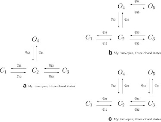
Examples for Markov models.

Whether a channel is open or closed is usually represented in the model by more than one state, i.e., several S_i may correspond to one event O or C. Thus, the likelihood of a given sequence of events (E^k) cannot be calculated without knowing the sequence (M^k) of corresponding model states. The approach followed here for overcoming this difficulty is the construction of a probability distribution P((M^k)|(E^k),Q) from which a realization (M^k) will be sampled. Fig. S1 in the Supporting Material shows the processing of data points I via events E to model states M.

The graph of a Markov model is represented in matrix form by the infinitesimal generator Q = (q_ij), i, j = 1, …, n_S. In this matrix Q, each q_ij is the value of the transition rate from the state S_i to S_j or zero if the two states are not connected. The model is assumed to be conservative; i.e., for the diagonal elements q_ii, we have

$$q_{ii}=-\sum _{j\ne i}{q}_{ij},i=1,\dots ,n_S.$$ (2)

The initial distribution p₀ specifies the probabilities of the Markov model being in any of the states S₁, …, S_nS at time t = 0. Therefore, p₀ must be a stochastic vector whose nonnegative components sum to 1, i.e.,

$$p_0\in {\mathcal{P}}^{n_S}=\left\{p\in {\mathbb{R}}^{n_S}|\sum _{i=0}^{n_S}{p}_i=1,0\le p_i\le 1\right\}.$$ (3)

Starting from the initial distribution p₀, the time course of the probabilities p(t) is obtained as the solution of the differential equation

$$\frac{dp\left(t\right)}{dt}=p\left(t\right)Q,p_0\in {\mathcal{P}}^{n_S},$$ (4)

which is given by

$$p\left(t\right)=p_0\exp \left(Qt\right),$$ (5)

where exp denotes the matrix exponential. In most cases, we need transition probabilities from a state S_i to a state S_j during a sampling interval τ. Therefore, we define

$$A_{\tau }=\exp \left(Q\tau \right)=\left({\rho }_{ij}\right),i,j=1,\dots ,n_S.$$ (6)

For large t, the probability p(t) tends to the stationary distribution

$$\pi ={\lim }_{t\to \infty }p\left(t\right),$$

which can be calculated from Eq. 4 by solving the system of linear equations

$$\begin{array}{l}\pi Q=0,\hfill \\ \sum _{i=1}^{n_S}{\pi }_i=1.\hfill \end{array}$$ (7)

Under the assumption that the Markov model is at equilibrium, the detailed balance conditions hold, which are given by

$${\pi }_i{q}_{ij}={\pi }_j{q}_{ji},i,j=1,\dots ,n_S.$$ (8)

If the graph which is represented by Q is acyclic, Eq. 8 is automatically fulfilled.

Bayesian framework

For a continuous-time Markov model with infinitesimal generator Q, the rate constants are to be estimated from a sequence of events (E^k). Whether a model with a given matrix Q is a good or a bad representation of the data is expressed by the conditional probability P(Q|E). This probability is not evaluated directly. Instead, we consider

$$\mathbb{P}\left(Q|E\right)=\sum _{M\in \mathcal{M}}\mathbb{P}\left(Q,M|E\right),$$ (9)

where M is the set of all possible sequences of model states

$${\left(M^k\right)}_{k=1}^N$$

of length N; the probability of a sequence E of open and closed events is thus determined by taking into account all realizations of Markov states M ∈ M. Equation 9 can be further refined to explicitly include the influence of the stationary distribution π if P(Q,M|E) is replaced by P(π,Q,M|E). Of course, the evaluation of P(Q,M|E) for all M is infeasible in practice for large lengths N. Instead, we take advantage of M as an auxiliary variable which, eventually, will enable us to generate samples for Q from P(Q,M|E). The transition probabilities from a Markov state M^k to the next state M^k+1 are available from the matrix A_τ (see Eq. 6); therefore, the probability

$$\mathbb{P}\left({\left(M^k\right)}_{k=1}^N|{\left(E^k\right)}_{k=1}^N,Q\right)$$

can be calculated iteratively. Due to the Markov property, the transition probability to the state Mⁱ⁺¹ depends only on the current state M_i. Thus, we have

$$\begin{array}{l}\mathbb{P}\left({\left(M^k\right)}_{k=1}^N|{\left(E^k\right)}_{k=1}^N,Q\right)=\mathbb{P}\left(M^1|E^1,Q\right)\cdot \hfill \\ \prod _{i=1}^{N-1}\mathbb{P}\left(M^{i+1}|M^i,\left(E^1,\dots ,E^{i+1}\right),Q\right),M^i\in S.\hfill \end{array}$$ (10)

Equation 10 is the most important part of our algorithm because it will be used not only to generate realizations M but also for sampling Q. (See section 1 of the Supporting Material for an algorithm for generating (M^k) from this probability distribution.)

In the following, we define prior distributions for the rate constants of a model Q as well as for its stationary distribution π. Note that whereas the prior for the rate constants will be used for both MCMC algorithms MH and MHG which will be introduced in the next section, the prior for π will only be used for the MHG algorithm. The prior probability P(Q) is chosen to capture the assumption that rate constants of a model Q cannot have arbitrarily large values. This is ensured by an exponential prior

$$\mathbb{P}\left(Q\right)\propto \exp \left(\frac{Tr\left(Q\right)}{\lambda }\right),\lambda \in {\mathbb{R}}^{+},$$ (11)

where

$$Tr\left(Q\right)=\sum _{i=1}^{n_S}{q}_{ii}$$

is the trace of the matrix Q. Here and in the following, the symbol ∝ will be used if left- and right-hand sides are equal up to a multiplicative constant. Equation 11 assigns a low probability should rate constants be much larger than λ (we used λ = 30 ms⁻¹). Explorations of different values for λ suggest that the algorithm is relatively insensitive to this parameter. Only if very low values, say λ = 0.03 ms⁻¹, are chosen, the influence of the prior becomes so strong that some test data sets are not fitted correctly; in this case, rate constants with values above 1 are assigned decreased values in the fit. However, this behavior was expected and merely demonstrates that the prior adequately serves its purpose.

For the stationary distribution π, we choose the Dirichlet density prior

$$\mathbb{P}\left(\pi \right)=\prod _{i=1}^{n_S}{\pi }_i^{b_i-1}\left\{\Gamma \left(\sum _{i=1}^{n_S}{b}_i\right)/\prod _{i=1}^{n_S}\Gamma \left(b_i\right)\right\},$$ (12)

where Γ is the gamma-function

$$\Gamma \left(z\right)={\int }_0^{\infty }{t}^{z-1}{e}^{-t}dt.$$ (13)

The hyperparameters b_i are assigned low values (b_i = 10⁻⁶) to obtain an uninformative prior. The choice of the prior Eq. 12 may seem arbitrary. In fact, the main motivation is the idea that, conveniently, together with the corresponding likelihood which will be defined below, π is distributed according to a Dirichlet distribution which can be sampled from directly. This strategy of choosing a conjugate prior was introduced by Raiffa and Schlaifer (32).

Methods

In this section, we develop Markov chain Monte Carlo (MCMC) methods for sampling sequences of model states M and models Q from the probability distribution P(M,Q|E). Two algorithms will be presented, one of which samples the full set of rate constants whereas the second version finds the stationary distribution π and half of the rate constants which together determine the remaining rates.

A Metropolized Gibbs sampler

Our goal is to sample from the probability distribution P(M,Q|E), i.e., we will generate a sequence of pairs

$${\left(M\left(l\right),Q\left(l\right)\right)}_{l=1}^L$$

(where L is the number of iterations). This can be achieved by alternating sampling from the conditional distributions

$$M\left(l\right)\sim \mathbb{P}\left(M|Q\left(l\right),E\right),$$ (14)

$$Q\left(l\right)\sim \mathbb{P}\left(Q|M\left(l-1\right),E\right),$$ (15)

instead of sampling directly from P(M,Q|E). This is an example of the Gibbs sampler (33), one of the classical MCMC algorithms.

To sample a realization of model states M as in Eq. 14, the probability distribution P(M|E,Q) has to be calculated using Eq. 10. Then, the sequence M can be sampled iteratively with a variant of the well-known forward-backward algorithm (34) (details can be found in the Supporting Material). Sampling Q from Eq. 15 requires an additional Metropolis-Hastings step (35,36), which is the reason why our algorithm is called a Metropolized Gibbs sampler.

Sampling of all rate constants (MH)

Unfortunately, it is not possible to sample Q directly from P(M,Q|E), but it shows that P(M,Q|E) can instead be calculated by evaluating Eq. 10 and the prior P(Q) from Eq. 11:

$$\mathbb{P}\left(Q|M,E\right)\propto \mathbb{P}\left(M|Q,E\right)\mathbb{P}\left(Q\right).$$ (16)

Now, from a given Q, a new sample $\tilde{Q}$ can be generated in two steps using a Metropolis-Hastings algorithm (35,36).

First, we generate a proposal $\tilde{Q}=\left({\tilde{q}}_{ij}\right)$ by changing the set of rate constants

$${\tilde{q}}_{ij}=\{\begin{array}{ll}{q}_{ij}+u_{ij},\hfill & \text{i}\text{f}{q}_{ij}>0,u_{ij}\sim U\left(-\delta ,\delta \right),\hfill \\ 0,\hfill & \text{i}\text{f}{q}_{ij}\le 0,\hfill \end{array}$$ (17)

where U(−δ, δ) is the continuous uniform distribution on the interval [−δ, δ]. Of course, after applying Eq. 17 the matrix $\tilde{Q}$ must be adapted so that Eq. 2 and Eq. 8 hold.

In a second step, it has to be decided whether the proposal generated by Eq. 17 is accepted as a sample from the probability distribution P(M,Q|E). The model $\tilde{Q}$ is accepted with probability

$$\alpha =\min \left\{1,\frac{\mathbb{P}\left(\tilde{Q}\right)\mathbb{P}\left(M|\tilde{Q},E\right)}{\mathbb{P}\left(Q\right)\mathbb{P}\left(M|Q,E\right)}\right\},$$ (18)

where the right-hand sides of evaluating Eq. 16 for Q and $\tilde{Q}$ appear in the quotient. Equation 18 shows that a proposal $\tilde{Q}$ is accepted for sure if its likelihood is greater than for the sample Q.

Rate constants and stationary distribution (MHG)

The detailed balance conditions, Eq. 8, allow for an alternative to Metropolis-Hastings sampling of all rate constants: If the stationary distribution π can be determined, only half of the rate constants—say, for example, the subdiagonal rates q_ij with i > j—have to be sampled using Eqs. 17 and 18. The remaining rate constants can then be calculated by Eq. 8. Adding an additional Gibbs step for sampling π requires only minor changes: Eq. 16 is replaced by

$$\mathbb{P}\left(Q|\pi ,M,E\right)\propto \mathbb{P}\left(M|\pi ,Q,E\right)\mathbb{P}\left(Q\right)\mathbb{P}\left(\pi \right),$$ (19)

which indicates that an additional prior P(π) (Eq. 12) is required.

Assuming that the conditional probability of π only depends on the sequence of model states M, we obtain

$$\pi \left(l\right)\sim \mathbb{P}\left(\pi |M\left(l\right),Q\left(l\right),E\right)=\mathbb{P}\left(\pi |M\left(l\right)\right).$$ (20)

The likelihood $\mathbb{P}\left(\pi \right|M)$ can be modeled by a Dirichlet distribution

$$\mathbb{P}\left(\pi |M\right)={\mathcal{D}}_{n_S-1}\left(S_1\left(M\right),\dots ,S_{n_S}\left(M\right)\right),$$ (21)

where S_i(M) gives the number of occurrences of the state S_i in the sequence M. This choice of P(π|M) gives the correct distribution for π if each component π_i is binomially distributed B(N,π_i) where N is the length of the sequence M. This is true provided that the Markov chain is at equilibrium. With the prior defined above (see Eq. 12), π can be sampled from the Dirichlet distribution

$$\pi \sim {\mathcal{D}}_{n_S-1}\left(G\left(M\right)\right)$$ (22)

with

$$G_i\left(M\right)=S_i\left(M\right)+b_i.$$ (23)

Results

The two MCMC methods MH and MHG, which were developed in the preceding sections, will now be applied to test data which was generated from a Markov model. The samplers are compared with earlier algorithms by Gin et al. (23) and Rosales and co-workers (19,20). Finally, we demonstrate how our algorithm performs on single-channel data collected from an inositol trisphosphate receptor.

Testing the method

First, we apply the method to test data which has been generated from model M₂ (see Fig. 1 b), a Markov model with two open and three closed states. A trace of 2000 ms is simulated using the Gillespie algorithm (37) for the parameters given in Table 1.

Table 1.

Parameters for models M₁, M₂, and M₃ (see Fig. 1)

Model M1		Model M2		Model M3
q12 = 0.058	q21 = 0.3	q12 = 0.058	q21 = 0.3	q12 = 0.058	q21 = 0.3
q23 = 1.7	q32 = 0.6	q23 = 1.7	q32 = 0.6	q23 = 1.7	q32 = 0.6
q24 = 4.9	q42 = 0.8	q24 = 4.9	q42 = 0.8	q24 = 4.9	q42 = 0.8
		q45 = 0.3	q54 = 0.1	q35 = 0.3	q53 = 0.1

All values given in ms⁻¹.

If the model is in one of the two open states, a single channel current of L₁ = −20 pA is given; if in one of the closed states, the current is L₂ = 0 pA. Normally distributed white noise with a variance of σ² = 7.5 pA is added and the trace is sampled with a sampling time of 0.05 ms, thus each data set consists of 40,000 data points. Both MH and MHG sampler (after a burn-in time of 10,000 iterations) converge to distributions whose mean values are close to the correct rate constants (compare to Table 1). Histograms showing the results of the MHG sampler for all rate constants are presented in Fig. 2.

Figure 2.

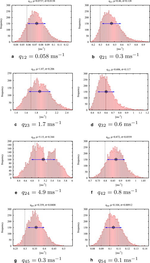
Histograms for the algorithm MHG after 50,000 iterations and a burn-in time of 10,000 iterations. MHG was run on a test data set consisting of 40,000 data points generated from model M₂ (see Table 1, M₂ columns). (Vertical dotted lines) True values of the rate constants. (Asterisks) Means of the histograms and (Arrows) standard deviations.

So far, we have demonstrated that our algorithm finds the correct set of rate constants from a given test data set if the graph of the Markov model which was used for generating the data is known. For single-channel data, it is not clear, however, how many open and closed states should be included in the Markov model and how they should be connected. The second part of this question is a difficult problem which cannot be discussed in full detail here. Although the possibilities for connecting open and closed states grow rapidly with the number of states, many of these seemingly different models are equivalent in the sense that they are capable of modeling the same dwell-time distributions. Thus, it is impossible to uniquely determine the model with the correct connections between open and closed states for a given data set because, almost always, several models which differ in the connections between states fit the data equally well. The reader is referred to Bruno et al. (38) for a more detailed discussion.

We will now demonstrate that our MCMC algorithm shows encouraging results if fits to overparameterized models are attempted: For this purpose, test data is simulated from model M₁ (Fig. 1 a) and fitted to the models M₂ and M₃ (Fig. 1, b and c), which have one more open state. If the MH sampler is used for fitting to model M₂, a typical convergence plot is shown in Fig. 3. Although the six rates q₁₂, q₂₁, q₂₃, q₂₄, q₃₂, and q₄₂ that are present in the correct model with only one open state tend to approximately correct values, it seems that the rates q₄₅ and q₅₄ wander around in a large range.

Figure 3.

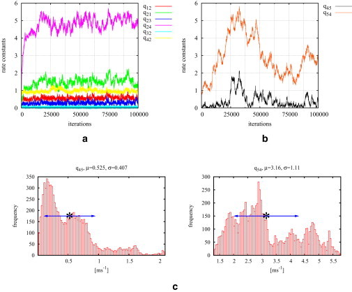
Model M₂ is fitted to test data of 40,000 data points generated from the simpler model M₁ using the MH sampler. The convergence plots (a and b) show that the rates connecting to the extra state O₅ wander around whereas the others tend to the correct values (compare this to Table 1, M₁ columns). Histograms for q₄₅ and q₅₄ are shown in panel c. The wide-spread multimodal posterior distributions for both rate constants clearly indicate that the state O₅ is not supported by the data.

The histograms for these two rate constants show a wide-spread multimodal distribution (see Fig. 3 c), which is another strong hint that the five-state model is not supported by the data. Thus, if a data set is fitted to a model consisting of too many states it is expected that not all rate constants will be fixed. Using the MH algorithm for fitting the same data set to model M₃ leads to even more promising results: Only after a few thousand iterations, the stationary probability of the extra-state O₅ tends to zero (see Fig. 4). This clearly shows that the algorithm detects that the state O₅ is superfluous.

Figure 4.

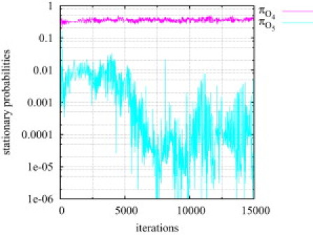
Model M₃ is fitted to test data (40,000 data points) generated from the simpler model M₁ using the MH algorithm. The stationary probability of the additional open state O₅ quickly tends to zero. This suggests that the sampler detects when a model is too complex for representing a given data set and reacts by switching off transitions to the additional state.

If MHG is used to fit data generated from M₁ with either M₂ or M₃, the stationary probability of the additional state O₅ tends to zero after only a few ten or hundred iterations; eventually, the algorithm terminates due to the criterion described in section 3 of the Supporting Material. Because under such circumstances MHG typically terminates after a few seconds, it can be used for a quick exploration of the number of states which a suitable model should have. Similar results are obtained for both algorithms when data generated from M₁ is fitted to other models which have more open states than M₁.

In summary, these results suggest that our algorithm behaves appropriately if the model which was chosen for fitting is too complex for representing a given data set. In future, reversible jump MCMC (39) and stochastic variable selection could be used to discriminate different models on a more formal basis.

Comparison with the method by Rosales et al. (19)

The performance of both methods is compared for a test data set of 100,000 data points at a sampling interval of τ = 0.05 ms generated from model M₂ shown in Fig. 1. In contrast to our algorithm, the Gibbs sampler by Rosales et al. (19) estimates transition probabilities during the sampling interval τ, i.e., the matrix A_τ = exp(Qτ) rather than the matrix of rate constants Q. With our own implementation of the Gibbs sampler by Rosales et al. (19), an estimate A_τ^G is computed while we use both versions of our algorithm for calculating estimates Q^MH and Q^MHG, respectively.

From each of these samples, we calculate the matrix exponentials A_τ^MH and A_τ^MHG so that the probability distribution of the true matrix exponential A_τ is obtained. In Fig. 5, representative examples for histograms of A_τ^G and A_τ^MH can be compared. Fig. 5 b shows that, especially, smaller entries of A_τ are generally overestimated by Rosales' algorithm. This is also demonstrated quantitatively in Table S1 which can be found in the Supporting Material.

Figure 5.

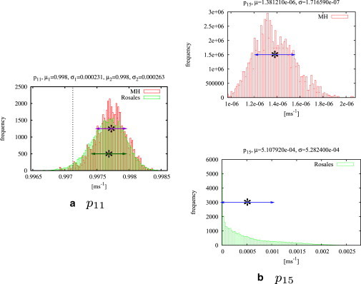
Rosales' Gibbs sampler and the MH algorithm are compared for a test data set of 100,000 data points. As representative examples, we show histograms for components ρ₁₁ and ρ₁₅ of the matrix exponential A_τ (plotted in red) of model M₂ (see Fig. 1) with results from Rosales' Gibbs sampler (plotted in green). (Vertical dotted line) Exact value of the matrix component. Both methods give very similar results for the diagonal of A_τ, as can be seen in panel a, for example. Mean and standard deviations for MH algorithm (purple) and Rosales' Gibbs sampler (green) are similar. The histograms for the off-diagonal elements found by Rosales' method are distributed over a wide range and are therefore much less accurate than the estimates found by MH; compare the two fits for ρ₁₅ in panel b.

Comparison with the method by Gin et al. (23)

As our proposed new approach, the method described by Gin et al. (23, section 2.5), estimates the rate constants of a Markov model Q but the algorithm depends on the fact that either the open or the closed state of the ion channel can be represented by a single Markov state. Therefore, we use model M₁ with the set of rate constants from Table 1 (M₁ columns) for a comparison. The resulting rate constants are not very different; thus, results are not presented here. However, the method due to Gin et al. (23) is much more efficient because sampling a sequence (M^k) of Markov states is not necessary.

Comparison with the MLE technique by Qin et al. (3,4)

Maximum-likelihood estimators (MLEs) provide point estimates for the rate constants of a Markov model for a given data set. The uncertainty of these estimates is quantified by the variance which can be computed together with the MLEs. In contrast, MCMC makes available the full posterior distribution of a model depending on a given data set while, nevertheless, maximum likelihood estimators as well as other statistical parameters like the expected value and the variance can still be determined. Quantitative comparisons of MLE and MCMC are only possible by reducing the probability distributions obtained by MCMC to point estimates. Therefore, in principle, such a comparison disadvantages MCMC. Nevertheless, we will demonstrate that suitably chosen point estimates show similar accuracy as maximum likelihood estimators.

To show how the MCMC methods developed here perform in comparison with maximum likelihood estimation, we compare our results with the MLE technique presented in Qin et al. (3,4). It shows that MCMC sampling comes with a clearly higher cost: A typical MLE fit takes a few seconds on a standard PC whereas the MCMC methods developed in this article run for a few minutes up to some hours depending on the size of the data set. For example, the fit of a test data set which was used for comparing QuB-MIL (http://www.qub.buffalo.edu) and MHG took 2 h with a two-core Intel 3.06 GHz processor with 4 GB memory. If models with only one open or one closed state are fitted, the efficient algorithm from Gin et al. (23, section 2.5) can be used, which decreases the run time to seconds up to a few minutes. The reason for this is that generating a large set of samples from a likelihood requires more effort than finding its maximum with an optimization algorithm.

Fig. 6 compares results of the MHG algorithm with the module MIL of the QuB software (Ver. 1.5.0.29; http://www.qub.buffalo.edu), for a test data set generated from model M₂. The plots clearly demonstrate the advantages of full probability distributions as obtained from MCMC algorithms over point estimates: With a point estimate there will always be some doubt how well a model is supported by the data. If the marginal distributions for the rates showed more than one distinguished mode, this would indicate that more than one choice of parameters might be equally likely, which means that the model is not uniquely determined by the data. For Fig. 6, note that the distributions are clearly smooth and unimodal, which gives confidence that the model is appropriate.

Figure 6.

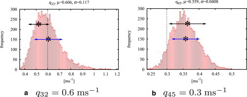
Selected histograms for a MHG run (50,000 iterations) and results of QUB-MIL for a test data set of 40,000 data points. (Dotted vertical line) The true value of a rate constant. (Asterisk) The maximum likelihood estimator found by QuB-MIL. (Upper arrows) Standard deviation found by QuB-MIL; (lower arrows) mean and standard deviations found by MHG. The estimates with relative errors are ${\widehat{q}}_{32}^{MIL}=0.522\left(-13.0\%\right),{\widehat{q}}_{32}^{MHG}=0.606\left(+1\%\right)$ and ${\widehat{q}}_{45}^{MIL}=0.365\left(+21.5\%\right),{\widehat{q}}_{45}^{MHG}=0.359\left(+19.7\%\right)$.

There are clear hints already during the fitting process, e.g., that some of the rate constants vary over a wide range, if we run MH or MHG with an overparameterized model. This leads to distributions for some rate constants which are spread over a wide range, and are multimodal or even close to uniform (see Fig. 3 c). MLE algorithms might still converge for an inappropriate model and the only indications for a fit failing to represent the data often are that the likelihood is not significantly higher or that the dwell-time histograms are not better approximated than for less complex models.

As well as MLE, MCMC approaches allow for ranking models by likelihoods which are obtained in our case from Eq. 16 or Eq. 19, respectively. Beyond that it was shown that additional, more qualitative information on the quality of the fit can be obtained from the probability distributions—information which is not available for MLE approaches or any other method which relies on point estimates.

Single-channel data

So far, the new MCMC algorithms have only been applied to test data. To give an idea how our approach can be used in practice, we conclude this section with a small example of fitting experimental data which was collected from an IP₃-type I receptor at a calcium concentration of 200 nmol/L (24). For experimental data, the required number of open and closed states is not known, although a lower bound can be obtained by the number of distinct maxima in the log-linear dwell-time histograms. As more and more states are added, our algorithms assign low stationary probabilities to superfluous states and thus allow for improving the fit without choosing an overparameterized model.

The main shortcoming of the method by Gin et al. (23) is that only fits to models with either one open or one closed state are possible whereas our methods allow for fitting models with arbitrary numbers of open and closed states. We fit a data set by Wagner et al. (24) with MH. The sampler converges for model M₁ as well as model M₂. To give a visual impression of the goodness of fit we show how well the empirical open time histogram is approximated by the fits to M₁ and M₂. Note that the algorithms presented here are not based upon estimated open and closed times. Thus, comparing the estimated dwell-time distributions with the histograms provides an independent test of the inferred model.

It has to be mentioned that dwell-time histograms can only be obtained by preprocessing from measurements which come in discrete multiples of the sampling interval τ, which severely distorts the histogram. For constructing the open time histogram shown in Fig. 7, a and c, open times were assumed uniformly distributed over a sampling interval as suggested by Gin et al. (23, section 2.3), and adjusted accordingly. Although the open time histogram has only one distinct maximum, it shows that the distribution obtained from the fit to the model with two open states approximates the histogram better for long open events (see Fig. 7, b and d). However, it seems that the theoretical open times distribution of model M₂ fits the empirical histogram less well for short events.

Figure 7.

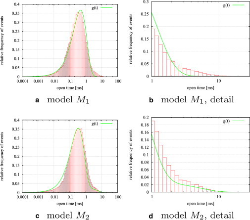
Open histogram for a data set of 1,400,000 data points which was collected from an IP₃-type I receptor at a calcium concentration of 200 nmol/L (24). This is shown together with the superimposed open time distributions determined by fits to two different models, one with one open state (M₁) and one with two open states (M₂) (see Fig. 1, a and b). Although the histogram has only one distinguished peak indicating that one open state is sufficient, it shows that the open time histogram is better approximated for long open events by the model with two open states.

Discussion

A new approach, to our knowledge, for estimating Markov models for ion channels was presented. It was demonstrated that both versions of the algorithm perform well on a test data set generated by M₂.

The algorithm presented here is a generalization of the approach developed by Gin et al. (23). This method allows for a very efficient implementation because probabilities for sequences of events (E^k) can be calculated without generating a sequence of corresponding Markov states (M^k), which is very time-consuming especially for large data sets. However, this approach is restricted to models where either open or closed events can be modeled by only one Markov state.

Rosales' Gibbs sampler (19–22) estimates a discrete Markov model which corresponds to the matrix A_τ. The advantage of this idea is that Gibbs sampling typically converges after just a few thousand iterations. However, due to difficulties with the computation of matrix logarithms, it is not easy to relate the estimated matrix A_τ to the infinitesimal generator Q of a continuous-time Markov model. In addition, in comparison with our algorithm, the Gibbs sampler was much less accurate. The reason for this is that the estimates of the transition probabilities ρ_mn from a state S_m to S_n are based upon counting the frequencies of this particular transition in the sequence (M^k). This works well for transitions which occur often but low transition probabilities are highly overestimated even if the sequence (M^k) is long. Our algorithms are not susceptible to these inaccuracies because the transition probabilities ρ_mn are not directly inferred from the observations. Rather, MH and MHG explore which infinitesimal generators Q could have generated the observed sequence of events (E^k).

In comparison with maximum likelihood estimators, MCMC methods generally require a longer runtime. The algorithms developed here are no exception. However, MCMC methods return probability distributions which give a more complete picture of the variability of parameters than any point estimate. The posterior distribution can be further explored for extraction of additional details such as correlations of two or more parameters, making it possible to investigate questions more subtle than estimating model parameters. Nevertheless, modes, expected values, and other statistical parameters can easily be calculated from MCMC samples. Therefore, MCMC makes better use of the experimental data than conventional methods because it extracts much more information.

In summary, MH and MHG combine ideas from earlier work by Rosales and co-workers (19,20) and Gin et al. (23). These ideas are extended by allowing for direct fitting to the rate constants of a Markov model for arbitrary numbers of open and closed states. The fits which we presented for data from the IP₃ receptor suggests that this is where most of the potential benefits of the prospectively new approach are. Although the data set has only one distinct maximum in the open time histogram, a fit to model M₂ which has two open states was successful. Comparison of the open time histogram of model M₂ shows that long events are better approximated by this model than by M₁, which has only one open state.

References

- 1.Neher E., Sakmann B. Single-channel currents recorded from membrane of denervated frog muscle fibers. Nature. 1976;260:799–802. doi: 10.1038/260799a0. [DOI] [PubMed] [Google Scholar]
- 2.Colquhoun D., Hawkes A.G. On the stochastic properties of single ion channels. Proc. R. Soc. Lond. B Biol. Sci. 1981;211:205–235. doi: 10.1098/rspb.1981.0003. [DOI] [PubMed] [Google Scholar]
- 3.Qin F., Auerbach A., Sachs F. Idealization of single-channel currents using the segmental K-means method. Biophys. J. 1996;70:MP432. [Google Scholar]
- 4.Qin F., Auerbach A., Sachs F. Maximum likelihood estimation of aggregated Markov processes. Proc. R. Soc. Lond. B Biol. Sci. 1997;264:375–383. doi: 10.1098/rspb.1997.0054. [DOI] [PMC free article] [PubMed] [Google Scholar]
- 5.Colquhoun D., Hawkes A.G., Srodzinski K. Joint distributions of apparent open and shut times of single-ion channels and maximum likelihood fitting of mechanisms. Philos. Trans. R. Soc. Lond. A. 1996;354:2555–2590. [Google Scholar]
- 6.Gamerman D., Lopes H.F. Texts in Statistical Science. 2nd Ed. Vol. 68. Taylor & Francis; Boca Raton, FL: 2006. Markov Chain Monte Carlo: Stochastic Simulation for Bayesian Inference. [Google Scholar]
- 7.Gilks W.R., Richardson S., Spiegelhalter D.J., editors. Markov Chain Monte Carlo in Practice. Chapman & Hall; London, UK: 1996. [Google Scholar]
- 8.Ball F.G., Cai Y., O'Hagan A. Bayesian inference for ion-channel gating mechanisms directly from single-channel recordings, using Markov chain Monte Carlo. Proc. R. Soc. Lond. A. 1999;455:2879–2932. [Google Scholar]
- 9.Sachs F., Neil J., Barkakati N. The automated analysis of data from single ionic channels. Pflugers Arch. 1982;395:331–340. doi: 10.1007/BF00580798. [DOI] [PubMed] [Google Scholar]
- 10.Roux B., Sauvé R. A general solution to the time interval omission problem applied to single channel analysis. Biophys. J. 1985;48:149–158. doi: 10.1016/S0006-3495(85)83768-1. [DOI] [PMC free article] [PubMed] [Google Scholar]
- 11.Blatz A.L., Magleby K.L. Correcting single channel data for missed events. Biophys. J. 1986;49:967–980. doi: 10.1016/S0006-3495(86)83725-0. [DOI] [PMC free article] [PubMed] [Google Scholar]
- 12.Ball F.G., Sansom M.S.P. Aggregated Markov processes incorporating time interval omission. Adv. Appl. Probab. 1988;20:546–572. [Google Scholar]
- 13.Milne R.K., Yeo G.F., Madsen B.W. Stochastic modeling of a single ion channel: an alternating renewal approach with application to limited time resolution. Proc. R. Soc. Lond. B Biol. Sci. 1988;233:247–292. doi: 10.1098/rspb.1988.0022. [DOI] [PubMed] [Google Scholar]
- 14.Yeo G.F., Milne R.K., Madsen B.W. Statistical inference from single channel records: two-state Markov model with limited time resolution. Proc. R. Soc. Lond. B Biol. Sci. 1988;235:63–94. doi: 10.1098/rspb.1988.0063. [DOI] [PubMed] [Google Scholar]
- 15.Crouzy S.C., Sigworth F.J. Yet another approach to the dwell-time omission problem of single-channel analysis. Biophys. J. 1990;58:731–743. doi: 10.1016/S0006-3495(90)82416-4. [DOI] [PMC free article] [PubMed] [Google Scholar]
- 16.Magleby K.L., Weiss D.S. Estimating kinetic parameters for single channels with simulation. A general method that resolves the missed event problem and accounts for noise. Biophys. J. 1990;58:1411–1426. doi: 10.1016/S0006-3495(90)82487-5. [DOI] [PMC free article] [PubMed] [Google Scholar]
- 17.Hawkes A.G., Jalali A., Colquhoun D. The distributions of the apparent open times and shut times in a single channel record when brief events cannot be detected. Philos. Trans. R. Soc. Lond. A. 1990;332:511–583. doi: 10.1098/rstb.1992.0116. [DOI] [PubMed] [Google Scholar]
- 18.Hawkes A.G., Jalali A., Colquhoun D. Asymptotic distributions of apparent open times and shut times in a single channel record allowing for the omission of brief events. Philos. Trans. R. Soc. Lond. B Biol. Sci. 1992;337:383–404. doi: 10.1098/rstb.1992.0116. [DOI] [PubMed] [Google Scholar]
- 19.Rosales R., Stark J.A., Hladky S.B. Bayesian restoration of ion channel records using hidden Markov models. Biophys. J. 2001;80:1088–1103. doi: 10.1016/S0006-3495(01)76087-0. [DOI] [PMC free article] [PubMed] [Google Scholar]
- 20.Rosales R.A. MCMC for hidden Markov models incorporating aggregation of states and filtering. Bull. Math. Biol. 2004;66:1173–1199. doi: 10.1016/j.bulm.2003.12.001. [DOI] [PubMed] [Google Scholar]
- 21.Rosales R.A., Fill M., Escobar A.L. Calcium regulation of single ryanodine receptor channel gating analyzed using HMM/MCMC statistical methods. J. Gen. Physiol. 2004;123:533–553. doi: 10.1085/jgp.200308868. [DOI] [PMC free article] [PubMed] [Google Scholar]
- 22.Rosales R.A., Varanda W.A. Allosteric control of gating mechanisms revisited: the large conductance Ca2+-activated K+ channel. Biophys. J. 2009;96:3987–3996. doi: 10.1016/j.bpj.2009.02.042. [DOI] [PMC free article] [PubMed] [Google Scholar]
- 23.Gin E., Falcke M., Sneyd J. Markov chain Monte Carlo fitting of single-channel data from inositol trisphosphate receptors. J. Theor. Biol. 2009;257:460–474. doi: 10.1016/j.jtbi.2008.12.020. [DOI] [PubMed] [Google Scholar]
- 24.Wagner L.E., II, Joseph S.K., Yule D.I. Regulation of single inositol 1,4,5-trisphosphate receptor channel activity by protein kinase A phosphorylation. J. Physiol. (Lond.) 2008;586:3577–3596. doi: 10.1113/jphysiol.2008.152314. [DOI] [PMC free article] [PubMed] [Google Scholar]
- 25.Gin E., Wagner L.E., II, Sneyd J. Inositol trisphosphate receptor and ion channel models based on single-channel data. Chaos. 2009;19:037104. doi: 10.1063/1.3184540. [DOI] [PMC free article] [PubMed] [Google Scholar]
- 26.Ball F.G., Sansom M.S.P. Ion-channel gating mechanisms: model identification and parameter estimation from single channel recordings. Proc. R. Soc. Lond. B Biol. Sci. 1989;236:385–416. doi: 10.1098/rspb.1989.0029. [DOI] [PubMed] [Google Scholar]
- 27.Fredkin D.R., Rice J.A. Bayesian restoration of single-channel patch clamp recordings. Biometrics. 1992;48:427–448. [PubMed] [Google Scholar]
- 28.Fredkin D.R., Rice J.A. Maximum likelihood estimation and identification directly from single-channel recordings. Proc. Biol. Sci. 1992;249:125–132. doi: 10.1098/rspb.1992.0094. [DOI] [PubMed] [Google Scholar]
- 29.de Gunst M.C.M., Künsch H.R., Schouten J.G. Statistical analysis of ion channel data using hidden Markov models with correlated state-dependent noise and filtering. J. Am. Stat. Assoc. 2001;96:794–804. [Google Scholar]
- 30.Venkataramanan L., Sigworth F.J. Applying hidden Markov models to the analysis of single ion channel activity. Biophys. J. 2002;82:1930–1942. doi: 10.1016/S0006-3495(02)75542-2. [DOI] [PMC free article] [PubMed] [Google Scholar]
- 31.The Y.-K., Timmer J. Analysis of single ion channel data incorporating time-interval omission and sampling. J. Roy. Soc. Interface. 2006;3:87–97. doi: 10.1098/rsif.2005.0078. [DOI] [PMC free article] [PubMed] [Google Scholar]
- 32.Raiffa H., Schlaifer R. Harvard University Graduate School of Business Administration; Boston, MA: 1961. Applied Statistical Decision Theory. [Google Scholar]
- 33.Gelfand A.E., Smith A.F.M. Sampling-based approaches to calculating marginal densities. J. Am. Stat. Assoc. 1990;85:398–409. [Google Scholar]
- 34.Carter C.K., Kohn R. On Gibbs sampling for state space models. Biometrika. 1994;81:541–553. [Google Scholar]
- 35.Metropolis N., Rosenbluth A.W., Teller E. Equation of state calculations by fast computing machines. J. Chem. Phys. 1953;21:1087–1092. [Google Scholar]
- 36.Hastings W.K. Monte-Carlo sampling methods using Markov chains and their applications. Biometrika. 1970;57:97–109. [Google Scholar]
- 37.Gillespie D.T. A general method for numerically simulating the stochastic time evolution of coupled chemical reactions. J. Comput. Phys. 1976;22:403–434. [Google Scholar]
- 38.Bruno W.J., Yang J., Pearson J.E. Using independent open-to-closed transitions to simplify aggregated Markov models of ion channel gating kinetics. Proc. Natl. Acad. Sci. USA. 2005;102:6326–6331. doi: 10.1073/pnas.0409110102. [DOI] [PMC free article] [PubMed] [Google Scholar]
- 39.Green P.J. Reversible jump Markov chain Monte Carlo computation and Bayesian model determination. Biometrika. 1995;82:711–732. [Google Scholar]
Associated Data
This section collects any data citations, data availability statements, or supplementary materials included in this article.