Why the Phylogenetic Regression Appears Robust to Tree Misspecification

Abstract

The phylogenetic comparative method uses estimates of evolutionary relationships to explicitly model the covariance structure of interspecific data. By accounting for common ancestry, the coevolution between 2 or more traits, as a response to one another or to environmental variables, can be studied without confounding similarities due to identity by descent. Because the true phylogeny is unknowable, an estimate must be used, introducing a source of error into phylogenetic comparative analysis that can be difficult to quantify. This manuscript aims to elucidate how tree misspecification is propagated through a comparative analysis. I focus on the phylogenetic regression under a Brownian motion model of evolution and consider the effect of local phylogenetic perturbations on the regression fit. Motivated by Felsenstein's method of independent contrasts, I derive a matrix square root of the phylogenetic covariance matrix that has an obvious phylogenetic interpretation. I use this result to transform the perturbed phylogenetic regression model into an ordinary linear regression in which one interpretable point has been affected. The simplicity of this formulation allows the contributions of data and phylogeny to be disentangled when studying the effect of tree misspecification. Consequentially, I find that branch length misspecification can be easily explained in terms of the reweighting of contrast scores between subtrees. An analytical consideration of this and other perturbations helps to explain why the phylogenetic regression appears generally to be robust to tree misspecification, and I am able to identify conditions under which the regression may not yield robust results. I discuss why soft polytomies do not meet these problematic conditions, leading to the conclusion that unresolved bifurcations should have only modest effects on the regression fit.

Comparative studies, dating back to Aristotle, have identified organismal trends by comparing the values of certain variables across a range of species (Sanford et al. 2002). Two thousand years later, the same technique of interspecific comparison helped inspire Charles Darwin to propose the theory of natural selection, thereby establishing the evolutionary basis of modern comparative, functional, and adaptive morphology and anatomy (Mayr 1982). Today, the evolutionary process itself is studied in detail, and comparative studies remain the primary means of investigation (Ridley 1983; Harvey and Pagel 1991). Contemporary analyses of comparative data are explicitly statistical (e.g., Felsenstein 1985), and the methods developed for evolutionary biology have diffused into conservation biology (Fisher and Owens 2004), anthropology (Nunn and Barton 2001), linguistics (Lass 1997), and more recently into human genetics and genomics (Oakley et al. 2005; Guo et al. 2007). These methods share the common goal of controlling for similarity due to identity by descent.

Species usually descend from common ancestors in a hierarchical fashion, leading to inherited similarities between closely related species. Similarity may also arise from selective pressures, which a comparative analysis aims to reveal; however, adaptation and heredity must first be disentangled (Felsenstein 1985; Harvey and Pagel 1991; Miles and Dunham 1992). This confounding is the subject of the phylogenetic comparative method in which evolutionary relationships are used to model the covariance structure of interspecific data (Hansen and Martins 1996). By explicitly accounting for the hierarchy of descent, these techniques can uncover residual similarity that may be evidence of historical coevolution or adaptation (Grafen 1992).

Evolutionary relationships are idealized by a phylogeny, typically a bifurcating tree representing the patterns of lineage branching over time produced by the true evolutionary history of the species under study. Quantitative variables observed across a range of related species can thus be considered as dependent realizations of a stochastic process defined on the phylogeny that relates them. In particular, for variables measured on a continuous scale, phylogenetic Brownian motion predominates as a model of realized similarity by descent (Cavalli-Sforza and Edwards 1967; Felsenstein 1973, 1985). Linear models built upon this Brownian motion framework retain a Gaussian error structure that incorporates as covariance the dependencies exerted by phylogenetic relationships (Martins and Hansen 1997).

The implementation of any phylogenetic comparative method is predicated on the acquisition of a phylogeny, which by definition is historical and unobservable (Felsenstein 1985). Because the true phylogeny is unknowable, an estimate must be used and various methods have been developed for tree reconstruction (reviewed in Felsenstein 2004). Crucially, analyses downstream of the reconstruction often treat the phylogeny as known rather than as an estimate. Doing so introduces a source of error that is difficult to quantify, underscoring the need for robust methodology. This manuscript seeks to explain why the prevailing methodology is indeed robust.

THE PHYLOGENETIC REGRESSION

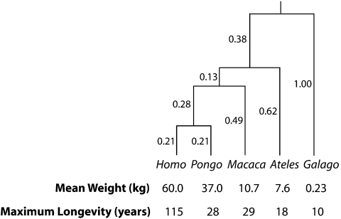
The phylogenetic comparative method encompasses a growing suite of procedures designed to draw inferences about evolution from interspecific data while accounting for the unusual statistical problem posed by phylogenetic history. Nevertheless, the minimal example of Figure 1 is sufficient to provide a conceptual understanding. The figure, adapted from Lynch (1991), illustrates a comparative data set in which measurements of 2 variables (mean species weight and maximum species longevity) are given for 5 species related by a presumptive phylogeny. A univariate regression model can be used to assess the relationship between mean weight and maximum longevity, but ordinary least squares (OLS) ignores the dependencies in the data imposed by the phylogeny. The role of the phylogenetic comparative method is simply to supply the dependence structure, with the goal of discounting the similarity by descent that is expected in data obtained from closely related species. In particular, phylogenetic Brownian motion assumes that the similarity by descent on each branch can be modeled by a shared additive component whose expected variance scales linearly with time. Consequently, the expected covariance for a pair of species is proportional to amount of evolution they share, calculated as the elapsed time (in total branch length) differentiating their common ancestor from the ultimate ancestor at the root of the phylogenetic tree.

FIGURE 1.

Phylogeny and data from 5 primate species. The 5 species (from left to right: Homo sapiens, Pongo pygmaeus, Macaca mulatta, Ateles geoffroyi, Galago senegalensis) are presumed to share a common ancestor 58 Ma. Branch lengths are reported as fractions of 58 million years. Below each species, its mean weight (in kilograms) and maximum longevity (in years) are shown. Example taken from Lynch (1991).

Returning to Figure 1, the Brownian motion covariance structure can be used in an interspecific regression of maximum longevity on mean weight (Felsenstein 1985, 1988). For such measurements, it is customary to log-transform both independent and dependent variables, leading to the model

(1)

where X and Y are the log-transformed variables, 1 is a vector of ones, 0 is a vector of zeros, ε∼N(0,σ²Σ), and the error covariance matrix Σ (sometimes called a phylogenetic covariance matrix or PCM) is defined by the phylogeny as

The intercept in Equation (1) is typically viewed as a nuisance parameter; conversely, β₁ is considered to be the “evolutionary regression coefficient” and quantifies the degree to which maximum longevity and mean weight have coevolved among the species in the study (Pagel 1993). As is true in all such applications of the phylogenetic comparative method, the parameter of interest β₁ in this example depends on the error covariance matrix Σ. Σ, in turn, depends on the phylogeny of Figure 1, which itself is often an estimate based on data external to the current analysis. Understanding how uncertainty and inaccuracy in phylogenetic reconstruction propagates into linear model estimation has been the subject of intense numerical study (Martins and Garland 1991; Purvis et al. 1994; Diaz-Uriarte and Garland 1996, 1998; Martins 2000; Martins et al. 2002; Symonds 2002). Here, I develop a complementary theory that formalizes how the phylogenetic regression is impacted by a misspecified tree.

PHYLOGENY AND THE PHYLOGENETIC REGRESSION

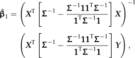
This study begins in consideration of the Model (1). In particular, I focus on the error covariance structure because it is Σ that translates phylogeny into the statistical model. It is worth emphasizing here that although Σ is often introduced as a covariance matrix between the observations Y, it is correctly the covariance matrix between the error terms ε. With respect to the observed data, Σ can be seen as the covariance matrix between the observations Y after conditioning upon both X and the unobserved value of the dependent variable (Y) at the root of the tree. The theory of generalized least squares (GLS) regression provides a means of expressing of the GLS estimate of β₁ in Equation (1) in terms of the error covariance matrix Σ. Specifically,

(2)

and here I focus on how varies with Σ. Rohlf gives an excellent discussion of the broad consequences of incorrectly specifying Σ. In particular, he notes that while the estimate will vary with Σ for any sample data set, in expectation it remains unbiased (see also Pagel 1993; Rohlf 2001). Indeed, Equation (2) specifies exactly how will vary with Σ for fixed X and Y (Rohlf 2006), but it does not lend insight into how prescribed changes to Σ translate into changes in . That is the goal of this manuscript: obtaining a meaningful and intuitive understanding of how prescribed changes to Σ translate into changes in for fixed X and Y.

To begin, rewrite the Model (1) as

(3)

by collecting the intercept β₀ and slope β₁ in a vector β and by appending 1 to X to create the predictor matrix . Having done this, for any invertible matrix square root B of Σ that satisfies BB^T = Σ, multiplication through Equation (3) by B ^{− 1} yields the transformed model

(4)

Crucially, B ^{− 1}ε∼N(0,σ²I), so that transformation by B ^{− 1} removes the error covariance structure and reduces the model to a less complicated OLS regression. The simplicity gained in the OLS reformulation does, however, come at a cost: unlike Σ, the structures of B and B ^{− 1} need not be interpretable in terms of the phylogeny. Several such B are implicit in the literature as means of reformulating the GLS Model (1) as an OLS Model (4), including those obtained from Σ through Cholesky decomposition (Butler et al. 2000), singular value decomposition (Garland and Ives 2000), and eigendecomposition (Rohlf 2001). Here, I focus on the eigendecomposition Σ = USU^T both to illustrate what it means for B and B ^{− 1} (in this case, analogous to US^1/2 and S ^{− 1/2}U^T, respectively) to be interpretable in terms of the phylogeny and to motivate the subsequent derivation of just such matrices. In addition to being illustrative, the choice of eigendecomposition is a historical one, as Cavalli-Sforza and Piazza (1975) established deep relationships between the branching pattern of a phylogeny and the eigenvectors of its corresponding covariance matrix (i.e., the columns of U). Indeed, these relationships have already found use in the phylogenetic comparative method, for example, in the study of phylogenetic shape by Martins and Housworth (2002). However, because the eigenvectors of Σ do not consistently mirror the phylogenetic branching pattern, the matrix square root B = US^1/2 is not well suited to my purposes here. To see this, consider the phylogeny of Figure 1, which is simple in every respect, being small, regularly shaped, and ultrametric. The matrix Σ admits the eigendecomposition Σ = USU^T, where

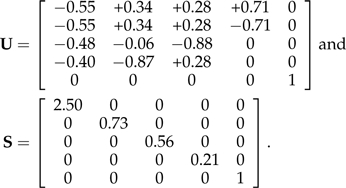Previous studies relating Σ to the branching structure of its corresponding phylogeny have relied upon clustering the signs of the entries in each but the last column of U (Martins and Housworth 2002). The fourth column of U, for example, clearly represents the Homo/Pongo clade (i.e., subtree), with the opposite signs of Homo ( + 0.71) and Pongo ( − 0.71) indicating their placement on opposing sides of the clade's common ancestor. The remaining columns, however, are less interpretable; by the same logic, the third column of U suggests that Homo ( + 0.28), Pongo ( + 0.28), and Ateles ( + 0.28) form a clade that shares a common ancestor with Macaca ( − 0.88), but this does not recapitulate the phylogeny (see Fig. 1). As a result, the transformed variables S ^{− 1/2}U^TX and S ^{− 1/2}U^TY that would be obtained in Equation (4) lack a direct phylogenetic interpretation.

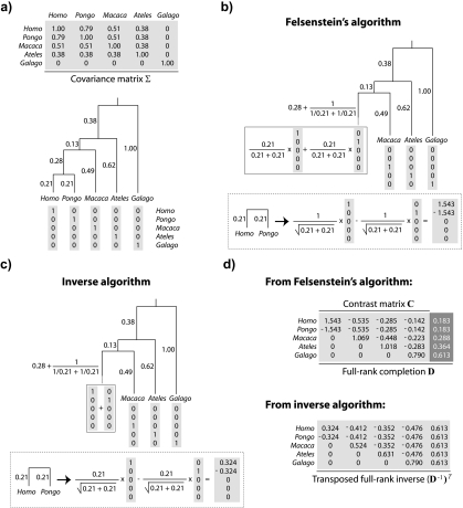
Fortunately, a suitable alternative to eigendecomposition was given implicitly by Felsenstein in his seminal work on the phylogenetic comparative method (Felsenstein 1973, 1985). Figure 2 depicts 2 algorithms for the matrix decomposition of Σ that operate in linear time. The first, Felsenstein's method of independent contrasts, has been modified to yield a nonsingular matrix D that satisfies D^TΣD = I; the second, which I call the inverse algorithm, is so named because it produces a matrix B that is the transpose of D ^{− 1}. Note that the matrix B satisfies BB^T = Σ and thus B is analogous to the U (or scaled to US^1/2) obtained by eigendecomposition (Rohlf 2001). The brief description of Felsenstein's algorithm that follows helps to explain why the decomposition of Figure 2 succeeds, where eigendecomposition fails. For a more complete description that motivates the algorithm, please see Felsenstein (1985) or Rohlf (2001).

FIGURE 2.

Two algorithmic decompositions of a phylogenetic covariance matrix. a) The phylogeny of Figure 1 and its associated covariance matrix Σ. Each leaf of the tree identifies with a vector chosen from the columns of the identity matrix. b) Matrix representation of Felsenstein's algorithm (Felsenstein 1973, Felsenstein 1985). In each of n − 1 iterations, 2 leaves sharing an immediate common ancestor (e.g., Homo and Pongo) are combined. The consequences of doing so are 3-fold: 1) a contrast is constructed as a weighted difference of the 2 leaf-associated vectors (see the first column of C in panel (d)); 2) a new leaf replaces the combined pair and is identified by a weighted sum of the 2 leaf-associated vectors; and 3) the branch adjacent to the new leaf is lengthened. c) The inverse algorithm. As in b, pruning occurs, resulting in a new leaf whose adjacent branch is lengthened; however, the weighted sums and differences of the 2 vectors comprising the cherry are different and constructed as shown. d) Square roots of C and of its inverse. The contrast vectors from Felsenstein's algorithm form an n×(n − 1) matrix C that satisfies C^TΣC = I_{n − 1}; addition of a final column (, dark gray) yields a nonsingular matrix D that satisfies D^TΣD = I_n. The vectors from the inverse algorithm form an n×n matrix B that is in fact the transposed inverse of D.

Felsenstein's algorithm is an iterative procedure that operates on a rooted phylogeny. Each step begins with the identification of 2 leaves sharing an immediate common ancestor (e.g., Homo and Pongo in Fig. 2a) and ends with those leaves having been replaced by a single new leaf (see Fig. 2b). Suppose that the branch lengths from Leaf 1 (e.g., Homo) and Leaf 2 (e.g., Pongo) to the common ancestor are t₁ and t₂, respectively. Then the new leaf extends the branch that led to the common ancestor by a distance of . The data assigned to this leaf are a weighted average of the data at Leaf 1 and Leaf 2; specifically, if the data are Y₁ and Y₂ for Leaf 1 and Leaf 2, respectively, then the value is attached to the new leaf (see Fig. 2b). Finally, a contrast is formed from the data at the leaves that were replaced. This contrast is just the difference Y₁ − Y₂ or after scaling. Let Y be the data vector whose entries are the Y_i. Then the contrast vector created in this step is the vector c such that c^TY equals the scaled contrast (see Fig. 2b). In sum, one step of Felsenstein's algorithm creates a contrast between leaf pairs and returns a phylogeny with one fewer leaf. Note that what constitutes a leaf changes as the algorithm proceeds, so that (as above) a leaf may combine the data from multiple leaves in preceding steps. In this way, contrasts between leaf pairs become contrasts between clades, leading to the incorporation of more species in the later steps of the algorithm. The algorithm terminates when the final 2 leaves are used to create a contrast, and so the number of contrasts created is one less than the original number of leaves.

The nature of Felsenstein's algorithm and the inverse algorithm that mirrors it (see Fig. 2c,d) is such that the structures of B and B ^{− 1} are unequivocally faithful to the phylogeny, and as is clear from Figure 2, the signs of the entries in all but the last columns of B and (B ^{− 1})^T cluster to describe genuine splits in the tree. Thus, the matrix B is an intuitive link between a phylogeny and its covariance matrix, and it also serves as a link between interspecific data (e.g., X and Y in Model (1) and parameter estimation. The key lies in finding the right transformation: using B to form interpretable linear combinations of the data, the dependence structure in a phylogenetic linear model can be removed without hopelessly conflating the data and the phylogeny. Returning to Model (1), expressing the data in a basis of the columns of B yields the vectors B ^{− 1}X and B ^{− 1}Y in the transformed model

(5)

Recall from Figure 2 that B^T = D ^{− 1} so that D^T = B ^{− 1} as well. The Model (5), in terms of D, is

(6)

and D^Tε∼N(0,σ²I_n). Note that multiplying Equation (1) through by C^T, where C from Figure 2d is the contrast matrix formed of all but the last column of D, eliminates the intercept, yielding the regression through the origin

(7)

where e∼N(0,σ²I_{n − 1}) (Rohlf 2001). These transformed variables are exactly the phylogenetically independent contrasts (Felsenstein 1973, 1985) that are commonly used to estimate the evolutionary regression coefficient β₁ instead of equivalently appealing to Model (1) through GLS (Garland and Ives 2000; Rohlf 2001). Thus, in what follows, my conclusions about how tree misspecification affects the phylogenetic regression of Equation (1) equally pertain to the use of independent contrasts in Equation (7).

USING CONTRASTS TO UNDERSTAND THE PHYLOGENETIC REGRESSION

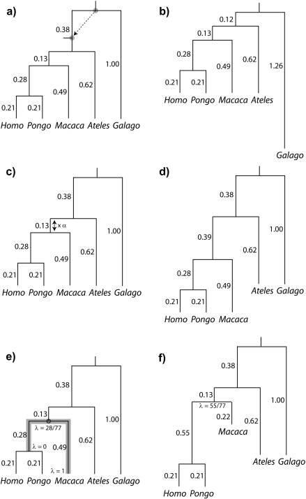
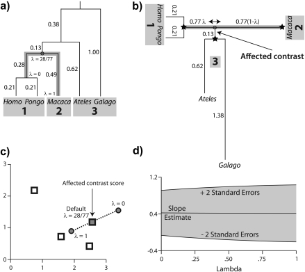
The previous section emphasized that the independent contrasts approach can be used to fully decompose phylogenetic covariance matrices in a manner consistent with branching structure. Here, I exploit the same contrast decomposition to study the effects of the tree misspecification on the phylogenetic regression. In what follows, I consider the impact of local misspecification by introducing small perturbations to a known phylogeny. These perturbations, which I call Equation (1) rerooting, Equation (2) branch scaling, and Equation (3) local regrafting, are illustrated in the 6 panels of Figure 3. Panels (a) and (b) show an example of rerooting, a perturbation that preserves both the branch lengths and the topology of the unrooted tree. In the figure, the root of the phylogeny from Figure 1 has been repositioned elsewhere on the tree. Panels (c) and (d) illustrate branch scaling, a perturbation that distorts the branch lengths but leaves the topology of the unrooted tree intact. Here, I have multiplied the length of one branch by a factor of α = 3, meaning that the length of the affected branch has been overestimated by a factor of 3 (estimated to be 0.39 instead of 0.13) Last, panels (e) and (f) depict local regrafting, a procedure that in effect chains together 2 particular branch scaling perturbations. The effect of local regrafting is to slide one subtree along a branch; in the figure, it is the Ateles/Galago subtree (i.e., the sliding subtree) that is free to slide along the branch connecting Macaca to the Homo/Pongo clade (i.e., the rigid subtrees).

In the context of phylogenetic linear models, the consequences of perturbing a tree as prescribed in Figure 3 are unclear, though simulation studies have considered the serial manipulation of specific phylogenies (Purvis et al. 1994; Diaz-Uriarte and Garland 1996, 1998; Abouheif 1999; Martins et al. 2002; Symonds 2002). Other studies interested in the effect of misspecification have addressed the consequences of using a randomly chosen tree (Martins 1996; Abouheif 1998) or simply ignoring the tree altogether (Rohlf 2006). In what follows, I apply the contrast decomposition to quantify the effects of small phylogenetic perturbations completely. Going forward, it should be noted that a series of local perturbations can be used to make global rearrangements, and that the changes described in Figure 3 can be used to deform any one tree into another. Thus, the insight gained from analyzing small perturbations extends to perturbations of any scale.

FIGURE 3.

Illustration of local perturbations, using the phylogeny introduced in Figure 1. Pairs of successive panels show the process (left) and the product (right) of the perturbation. a, b) The root is being repositioned elsewhere on the tree. c, d) The length of one branch is being scaled by a factor of α∈[0,∞]. As drawn in panel (d), α = 3. e, f) The subtree defined by Ateles and Galago is being regrafted elsewhere on the branch (shadowed in gray) connecting Macaca to the Homo/Pongo clade. The new graft site is parameterized by λ∈[0,1] in terms of distance from the Homo/Pongo clade as a fraction of total branch length (here 0.77). As drawn in panel (f), λ = 55/77.

REROOTING AND THE PHYLOGENETIC REGRESSION

To understand how tree misspecification in the form of a small perturbation influences the phylogenetic regression, I first consider how the perturbation affects the construction of independent contrasts. In particular, it is clear from Equation (7) that if the contrasts do not change then the regression equations do not change either. It is intuitive that repositioning the root on its branch has no effect on the construction of independent contrasts, as the following argument shows (see also Appendix 2). The rooted branch is the last to be considered in the contrast decomposition, and the influence of that branch is felt only through its length (i.e., κ in the appendix is a function of t₁ + t₂); repositioning the root on its branch maintains both the branch length and the order in which the contrasts are constructed, and as a consequence, the matrix C in Equation (7) is unchanged. More generally, it turns out that the root can be repositioned anywhere on the unrooted tree without affecting the phylogenetic regression. To see this, it suffices to consider the consequences of repositioning the root at either endpoint of its branch. Doing so creates a multifurcation and, as is widely appreciated, creates a choice of order in which the final contrasts are constructed. That is to say, when the root has been repositioned to an endpoint of its branch, Felsenstein's algorithm will generate a different contrast matrix C depending on the order in which the contrasts are resolved. Superficially, this appears to affect the phylogenetic regression through Equation (7), however, because these distinct contrast decompositions arise from a common tree, the underlying PCM Σ is the same. Thus, Equation (1) remains the same, making it clear that the choice of ordering will not affect the phylogenetic regression (see e.g., Garland and Diaz-Uriarte 1999). Collecting these observations, repositioning the root on its branch will not affect the regression slope, and by repositioning the root to an endpoint of its branch I can modify the order in which the contrasts are constructed. The effect of the latter is to “move” the root to an adjacent branch, and it has already been established that the root can be repositioned on its new branch without affecting the regression slope. It follows that rerooting the phylogeny leaves the regression slope unaffected, a feature that I will exploit in what follows.

BRANCH SCALING AND THE PHYLOGENETIC REGRESSION

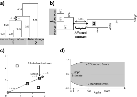
When a phylogeny has been misspecified, some combination of the branch lengths and the branching pattern are incorrect. In this section, I create misspecification by considering a local perturbation of branch length. To illustrate the approach, consider perturbing the phylogeny from Figure 1 as shown in Figure 3c,d. Here, a factor α is scaling the length of the branch (originally 0.13) that connects the Homo/Pongo/Macaca clade to the rest of the tree. Motivated by the previous section, my strategy is to place the root of the tree at the midpoint of the branch that is being perturbed. Upon doing so, the perturbed branch partitions the taxa into 2 descendant subtrees that have been labeled 1 and 2 in Figure 4a. The progressive decomposition of Σ as shown in Figure 2 defers consideration of the perturbed branch until the end (see also Appendix 2), and as a result, the contrast matrix C from Figure 2d and Equation (7) isolates the perturbed branch in its final column. Thus, the perturbed branch defines exactly one affected contrast, and it is this contrast that is emphasized in Figure 4b.

FIGURE 4.

Scaling the length of one branch by a factor of α. a) The split at the affected branch partitions the taxa into subtrees by separating the Homo/Pongo/Macaca clade (labeled 1) from Ateles and Galago (labeled 2). b) Each subtree is conceptually rooted at the proximal endpoint of the affected branch (indicated by black stars). Ancestral trait estimates are inferred at the root of each subtree, and the uniquely affected contrast is a scaled comparison of the 2 ancestral values. c) After rooting the tree on the affected branch, Felsenstein's algorithm yields 4 independent contrast scores (C_i^TX,C_i^TY), i = 1,2,3,4 (shown as squares): Homo versus Pongo, Homo/Pongo versus Macaca, Ateles versus Galago, and Homo/Pongo/Macaca versus Ateles/Galago. Only the last of these is a function of α (filled); the remaining 3 are invariant to the scale factor (hollow). The position of the affected contrast score in transformed coordinate space is constrained to be collinear with the origin (along the dotted line). Larger values of α decrease the importance of the affected contrast score in the linear regression by shifting its position toward the origin. d) The regression slope estimate is shown as α ranges from zero toward infinity on a logarithmic scale. Confidence bounds are given by the upper and lower curves that plot and, respectively (SE, standard error).

The affected contrast can be seen as a comparison of the 2 ancestral trait values estimated from the data private to each subtree. Note that because each subtree is rooted at the endpoint of the perturbed branch that lies closest to it, neither estimate is dependent on α. Instead, in scaling the distance in branch length between the 2 subtrees, α modifies the variance of the contrast between the ancestral traits imputed at either end of the affected branch. Figure 4c plots as squares the contrast scores (C_i^TX,C_i^TY), i = 1,2,3,4 to illustrate how α influences the data entering the phylogenetic regression. The coordinates of the affected contrast score (C₄^TX,C₄^TY) are shown both prior to perturbation (α = 1, shown as a filled square) and after introduction of the factor α (indicated by the dotted line). As α ranges from zero to infinity, the coordinates of the affected contrast score are drawn toward the origin along the dotted line. This is because the contrast between Homo/Pongo/Macaca and Ateles/Galago is maximally informative when their respective subtrees are drawn nearest to one another on the tree (i.e., scaling to zero, resulting in minimal variance) and minimally informative when their evolutionary histories are effectively independent (i.e., scaling to infinity, resulting in infinite variance).

As highlighted in Figure 4c, for the right set of contrasts, local branch length perturbation has a simple and interpretable effect. Moreover, what was a phylogenetic regression of Y on X with error covariance Σ can be seen through Equation (7) as an ordinary linear regression of C^TY on C^TX. Because this latter model lacks an intercept, the fitted regression line has slope and passes through the origin (Grafen 1992, Legendre and Desdevises 2009). Thus, the effect of the scale factor α depends primarily on the angle between the fitted regression line and the dotted line y = (C₄^TY/C₄^TX)x traversed by the affected contrast. When that angle is small, as is the case in Figure 4c, the scale factor has almost no impact on the regression. Figure 4d confirms this, revealing that neither nor its standard error is particularly sensitive to the choice of α. In general, for the perturbation of a single branch to strongly affect the phylogenetic regression, the affected contrast score must be able to exert substantial leverage and influence on the OLS regression fit.

BRANCH LENGTH ERROR IN GENERAL

As the previous section demonstrates, incorrectly specifying the length of one branch (equivalent to choosing an α≠1) has a limited effect on the phylogenetic regression. Moreover, the consequences of branch length overestimation (α > 1) and underestimation (α < 1) are not the same. Overestimation devalues the contrast across the affected branch (henceforth, the affected contrast) by shifting its coordinates toward the origin. Underestimation does the opposite, inflating the worth of the affected contrast in the regression by shifting its coordinates away from the origin. Importantly, the effect of branch length misspecification on the affected contrast is always linear, as the following technical presentation shows.

Building on the example of the previous section, I consider scaling the length of one branch in an arbitrary, possibly multifurcating phylogeny by a factor of α, where α is permitted to be either zero or infinity. Without loss of generality, the root can be repositioned anywhere on the branch that is being perturbed. I will suppose that the length of this branch prior to perturbation is t and that the root has been placed at its midpoint. By indexing the taxa appropriately, the covariance matrix of this rerooted phylogeny, Σ, can be written as

(8)

where each of Σ₁ and Σ₂ is a covariance matrix of the subtree(s) adjacent to one end of the rooted branch. Introducing the scale factor α gives us the perturbed covariance matrix

(9)

and the contrast vector that distinguishes the 2 has the form (see Appendix 2)

(10)

where

(11)

In the regression Model (7), the transformation of the (X,Y) data by this contrast vector yields the contrast score

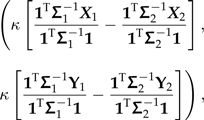(12)

where I use X_k and Y_k to denote vectors derived from X and Y that contain the data private to subtree k. It is this coordinate alone that is affected by the branch scaling perturbation through the scale factor κ (e.g., Fig. 4c). This point represents a contrast between the subtrees flanking the perturbed branch, and when α = 0, this contrast attains its maximum weight and influence on the regression. At the other extreme, as α tends to infinity, κ tends to zero, and the influence of this point on the slope of the regression line vanishes. Thus, the general effect of branch length errors can be understood in terms of the reweighting of contrast scores between subtrees. To the extent that the set of contrast scores computed across any branch of the tree is homogenous, the phylogenetic regression is expected to be robust.

LOCAL REGRAFTING AND THE PHYLOGENETIC REGRESSION

In this section, I consider the effect of removing a subtree and locally regrafting it onto the phylogeny. Operationally, the idea is to 1) choose a node on the tree, 2) choose a subtree adjacent to the node, and 3) slide the subtree along the branch that connects the remainder of the tree (see Fig. 3e,f). The version of local regrafting that I describe gently perturbs the tree by modifying the relative branch lengths at a junction of subtrees; the effect is to change the length of 2 adjacent branches while keeping the sum of their branch lengths constant. At the extreme, local regrafting induces a multifurcation, and through further sliding the branching pattern of the phylogeny can be arbitrarily deformed.

Recall from the discussion of branch scaling that after suitable rerooting the progressive decomposition of Σ deferred consideration of the perturbed branch until the end. The same holds true for the perturbation considered here; progressive decomposition can once again be used to isolate the effect of subtree sliding in one contrast vector. This time the root is placed at an internal node, so that the covariance matrix of this rerooted phylogeny can be written as

(13)

where Σ₃ + t₃1 represents the subtree that is to be locally regrafted and Σ₁ + t₁1 and Σ₂ + t₂1 represent the remaining subtrees at the newly positioned root. To capture the effect of sliding the subtree along its branch, I introduce the parameter λ and write the perturbed covariance matrix as

(14)

In other words, λ∈[0,1] indexes the relative position of the sliding subtree along the branch on which it resides, and the position prior to perturbation is given by (see Fig. 5a). As was the case in the previous section, only one contrast vector distinguishes Σ from Σ^*, and from Appendix 2 this contrast can be written as

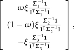(15)

where ω is a function of λ given by

(16)

and ξ is a function of λ given by

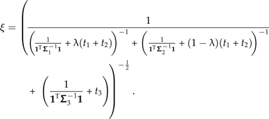(17)

FIGURE 5.

Locally regrafting a subtree. a) The sliding subtree (Ateles/Galago, labeled 3) meets the 2 rigid subtrees (Homo/Pongo, labeled 1; Macaca, labeled 2) at an internal node (hollow circle). Subtrees 1 and 2 are connected by a branch of total length 0.77; regrafting subtree 3 to this branch places it at a point 0.77λ and 0.77(1 − λ) units away from subtrees 1 and 2, respectively. b) Ancestral trait estimates are inferred at the root of each subtree as indicated by black stars. The value imputed at the hollow circle is a ω-weighted average of the estimates from subtrees 1 and 2 (see Equation (19)). The uniquely affected contrast is a scaled comparison of this weighted average to the ancestral trait estimate from subtree 3. c) After rooting the tree on the affected branch, Felsenstein's algorithm yields 4 independent contrast scores, only one of that is affected by λ (filled square; see Fig. 4c). The position of the affected contrast score in transformed coordinate space is determined by ξ and ω, both of that are functions of λ. ξ acts as a scale factor akin to α from branch scaling, whereas ω contributes a degree of nonlinearity to the trajectory of the affected contrast score (dotted line). d) The regression slope estimate is shown as λ ranges from zero to one. Confidence bounds are given by the upper and lower curves that plot and , respectively.

Thus, whereas the proximal effect of branch scaling was linear in the scale factor, the consequences of locally regrafting a subtree are evidently more complicated. This time, in the regression Model (7), the transformation of the (X,Y) data by the affected contrast vector yields the point

(18)

that includes ξ as a overall scale factor and ω as a weight on the relative contributions of Subtrees 1 and 2. Notice that for k = 1,2,3, the values and can be interpreted as estimates of the ancestral trait values using only the data from subtree k (see Fig. 5b). From this perspective, ω determines the relative contributions of the estimates from the 2 rigid subtrees in a contrast against the estimate obtained from the subtree that has been locally regrafted. This is one consequence of local regrafting; the relative position λ determines this relative contribution through its effect on ω. To clarify that effect, notice that the part of ω in Equation (17) that appears complicated, namely,

(19)

is really just a ratio of variances; the numerator and denominator are the variances in estimating trait values at the root using data private to Subtrees 1 and 2 (see Fig. 5b). Finally, recall that λ also appears in the scale factor ξ. This leads to a nonlinear dependence on λ because changing λ changes both how the affected contrast is computed and the weight that the contrast receives in the regression. Figure 5c indicates how the affected contrast score varies as λ ranges from zero to one. Because ω is close to one for all values of λ, the unstandardized value of the contrast (i.e., before multiplication by ξ) changes very little. By comparison, ξ is more sensitive to the choice of λ, leading to the nearly linear trajectory shown in the figure. This is similar to what was observed for branch scaling, and once again neither the slope estimate nor its standard error is greatly affected by the perturbation (Fig. 5d).

The formulas above extend beyond the example of Figure 5 to explain the general effects of local regrafting on the phylogenetic regression. For example, Equation (19) shows that the effect of λ on ξ is evidently negligible when is large, in other words, when there is substantial variance in estimating trait values from the sliding subtree. In that case, irrespective of λ, the affected contrast will not be very informative toward the estimation of β₁. Similarly, when t₁ + t₂, the length of the branch upon which the subtree slides, is small, ξ will also remain relatively unchanged. More interestingly, the formulas also reveal scenarios in which λ will have a major effect. Recall from the discussion of branch scaling that the effect of the scale factor α depends primarily on the angle between the fitted regression line and the line traversed by the affected contrast. Here, ξ plays a similar role, with ω contributing nonlinearity to the trajectory. This nonlinearity is exacerbated as ω deviates from unity, and it is clear from Equation (16) that large deviations are possible when and are both small. Broadly speaking, this scenario is most likely to occur when the affected branch lies deep in the phylogeny, for example, with branches near the root of an ultrametric tree. This may help explain why the simulations by Martins and Housworth (2002) and by Symonds (2002) revealed the phylogenetic regression to be particularly sensitive to topological changes near the root of the tree.

TOPOLOGICAL ERROR IN GENERAL

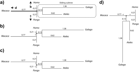
Because local regrafting, as depicted in Figure 5, acts only on one branch, a single regrafting step can create multifurcations but is insufficient to change the branching pattern of the phylogeny. In Figure 5b, for example, multifurcations occur when the sliding subtree reaches either extreme (λ = 0 or λ = 1), but to change the branching pattern of the tree requires further sliding beyond a multifurcation point. Figure 6 illustrates this further sliding, beginning from the multifurcation indexed by λ = 0 in Figure 5. This multifurcating tree, shown as unrooted in Figure 6a, can be resolved into an unrooted bifurcating tree by sliding theAteles/Galago subtree through the multifurcation point either upward (Fig. 6b), downward (Fig. 6c), or to the left (Fig. 6d). In each case, the distance that the sliding subtree has traversed beyond the multifurcation point is parameterized by ε. Significantly, the 3 bifurcating trees in Fig 6b–d have different branching patterns and thus unique sets of contrasts; viewed collectively, their corresponding regressions help to elucidate the consequences of topological error.

FIGURE 6.

Changing the tree topology by sliding a subtree through an internal node. a) The unrooted tree from Figure 5b is shown for λ = 0, at which point a multifurcation is present. Further sliding of the Ateles/Galago subtree either toward Homo (upward as in b) or toward Pongo (downward as in c), alters the topology of the tree. Sliding the subtree toward Macaca (left as in d) restores the topology of Figure 5. The branch leading to Macaca is shaded gray in panel (a) for consistency with Figure 5.

The effects of changing the branching pattern are shown in Figure 7a, which like Figures 4c and 5c plots contrast scores for a collection of phylogenetic regressions. Unlike the previous figures, however, 3 distinct branching patterns are being depicted at once. To accomplish this, each of the trees from Figure 6 has been rooted on the branch of length 0.13 that connects Ateles and Galago to the remainder of the tree. The rooted trees that result share 2 contrasts, the contrast between Ateles and Galago and the contrast between Ateles/Galago and Homo/Pongo/Macaca. The remaining 2 contrasts are unique for each tree and depend on the branching order or Homo, Pongo, and Macaca. Among those shared, the contrast between Ateles and Galago does not depend on ε and so the position of that contrast in Figure 7a is static. The remaining shared contrast depends strongly on ε; at the multifurcation point (ε = 0 in all 3 trees) the position of contrast between Ateles/Galago and Homo/Pongo/Macaca is the same (shown as a filled square), but as ε increases the positions for each tree diverge as illustrated by labeled arrows. Finally, the 2 contrasts private to each tree are invariant to ε, meaning that their positions are unique for each tree but remain static in the plot (points labeled b,c, and d according to the panels in Figure 6).

FIGURE 7.

The effect of changing the tree topology on the phylogenetic regression. a) After rooting the trees of Figure 6 arbitrarily on the branch of length 0.13, Felsenstein's algorithm yields 4 independent contrast scores for each of the trees in panels (b–d). The hollow square indicates the Ateles versus Galago contrast that is shared by the 3 topologies and invariant to choice of ε. The filled square indicates the Homo/Pongo/Macaca versus Ateles/Galago contrast that is shared by the 3 topologies but depends on ε. For ε = 0, the contrast scores coincide in transformed coordinate space; as ε increases, the position changes as indicated in by the labeled arrows and curves originating from the filled square (at ε = 0). Each of the trees in panels (b–d) additionally has 2 contrasts that are private to its topology and invariant to ε; the positions of the contrast scores are labeled by their respective panels. The dotted line indicates the phylogenetic regression line (y = 0.4377x) shared by all 3 trees at the multifurcation parameterized by ε = 0. b) The regression fits corresponding to the 3 trees in Figures 6b–d diverge as ε increases. Because the contrast score unique to Figure 6b has an upward trajectory relative to the ε = 0 regression line (see panel (a)), the estimated slope corresponding to that tree is increasing with increasing ε. Likewise, the estimated slope corresponding to the tree in Figure 6c decreases with increasing ε. Panel (a) shows that the trajectory of the contrast score unique to Figure 6d runs nearly parallel to the ε = 0 regression line; because of this, the slope does not change much as ε varies.

It is clear that when there is a multifurcation, the set of independent contrasts from Felsenstein's algorithm will not be unique (Felsenstein 1978, Purvis and Garland 1993). At the multifurcation parameterized by ε = 0, the trees in Figure 6b–d coincide even though as depicted in Figure 7 their contrast sets are different. Their common regression fit is shown in Figure 7a as a dashed line, and as ε increases the estimated regression slopes diverge (Fig. 7b). The manner of this divergence is intuitive from Figure 7a: the trajectory of the contrast that depends on ε indicates how the regression line will be torqued. An upward trajectory relative to the line, as occurs for the tree in Figure 6b, increases the estimated regression slope, whereas a downward trajectory (e.g., Fig. 6c) causes the slope to decrease. For the tree in Figure 6d, the trajectory is roughly parallel to the regression line, and as such the estimated slope changes little. Figure 7b illustrates the consequences of topological error as the branching pattern subtly varies. Transitions between topologies occur between ε > 0 on one line (e.g., the line labeled d) and ε > 0 on another line (e.g., the line labeled b). For the line labeled d, ε is proportional to λ from Figure 6, and the line itself is the slope estimate line from Figure 5d. Transitioning from ε > 0 on the line labeled d to ε > 0 on the line labeled b is equivalent to moving the sliding subtree from Figure 5 and Figure 6a past the multifurcation at λ = 0 and onto the branch leading to Homo. This underscores the point that 2 local regrafting steps are required to change the branching pattern of the tree, and it is through these steps that topological misspecification affects the phylogenetic regression. For any one such step, the factors that influence robustness were detailed above.

SOFT POLYTOMIES

The preceding discussions of errors in branch length and topology included cases when a truly bifurcating tree was misspecified as multifurcating. This type of error, known as soft polytomy, typically arises when there is insufficient data to resolve the local branching pattern at an internal node of the phylogeny (Maddison 1989). There has been significant interest in the effects of soft polytomy on comparative analyses (Grafen 1989, Grafen 1992; Pagel and Harvey 1992; Purvis and Garland 1993; Losos 1994; Diaz-Uriarte and Garland 1996, Diaz-Uriarte and Garland 1998; Martins 1996; Garland and Diaz-Uriarte 1999), and it is clear that these multifurcations occur at the extremes of both branch scaling (when α = 0) and local regrafting (when λ = 0,1). Thus, as a complement to simulation studies, the consequences of soft polytomy on the phylogenetic regression can be investigated using the machinery already introduced.

It is easiest to consider soft polytomy as the product of a branch scaling perturbation in which the length of a branch has been reduced to zero. As illustrated in Figure 4c, the effect of underestimating the length of one branch is to overvalue the contrast across the branch whose length is underestimated. If it is assumed that the branching pattern at the soft polytomy went unresolved because of insufficient data, it may be reasonable to assume that the unresolved branch length is small. Under that assumption, the degree to which the affected contrast is overvalued should be minor. This is clear from Equation (11): when the length of the unresolved branch, call it t, is small, the term in κ dominates αt for any α∈[0,1]. It follows that the affected contrast score will not change much, and thus the estimated regression slope will be only modestly affected.

DISCUSSION AND CONCLUSIONS

The widespread use of phylogenetic comparative methods, coupled with the dependence of these methods on an estimated phylogeny, has motivated the study of what can occur when the presumptive phylogeny is incorrect (Martins and Garland 1991, Purvis et al. 1994, Diaz-Uriarte and Garland 1996, Diaz-Uriarte and Garland 1998, Martins 2000, Martins et al. 2002, Symonds 2002). A number of simulation studies have demonstrated the phylogenetic regression to be generally robust to tree misspecification, but simulations alone cannot explain why this appears to be the case. Moreover, simulations rely on observations that may be specific to the data, to the phylogeny, to how the phylogeny is perturbed, or to some combination of the 3. As a complement to simulation, I have presented a theoretical approach that allows the data and the phylogeny to be disentangled. The results are general and help to explain why the phylogenetic regression appears to be robust to tree misspecification. I began this study by identifying the PCM Σ as a key intermediary between tree misspecification and its effect on the phylogenetic regression. Motivated by Felsenstein's method of independent contrasts (Felsenstein 1985), I derived a matrix square root of Σ that has an obvious phylogenetic interpretation and is minimally perturbed by small perturbations to a phylogeny. I used this result to transform the perturbed phylogenetic regression model into an ordinary linear regression in which one interpretable point has been perturbed. The simplicity of this formulation allowed us to disentangle the contributions of data and phylogeny when studying the effect of tree misspecification.

I considered the impact of local misspecification on the phylogenetic regression by introducing small perturbations to a known phylogeny. These perturbations, 1) rerooting, 2) branch scaling, and 3) local regrafting, were shown to have bounded influence on the regression fit. I discussed why rerooting has no effect on the slope estimate in a phylogenetic regression, and I used this result to reposition the root of the tree on the branch affected by the perturbation. In doing so, I was able to isolate and interpret the effects of branch scaling and local regrafting in terms of one affected contrast. The contrast affected by branch scaling represents a comparison between the subtrees flanking the perturbed branch. Overestimating the length of a branch decreases the influence of the contrast across that branch in the linear regression; conversely, underestimating the length of a branch gives its contrast undue influence. At the extreme, underestimating a branch length to be zero creates a soft polytomy in the estimated phylogeny. I have discussed why the effects of soft polytomy will be modest under the reasonable assumption that the length of the underestimated branch was actually small. Local regrafting targets a subtree of the unrooted phylogeny and causes it to slide along the branch to which it connects. This can be seen as a pair of branch scaling perturbations, and I have shown that the consequences of local regrafting and branch scaling are quantitatively similar. A multifurcation occurs through local regrafting when the targeted subtree slides to either end of the branch to which it connects. Further sliding through the multifurcation causes the branching pattern to change, and thus a pair of local regrafting perturbations is sufficient to deform the tree topology.

Throughout the manuscript, the discussion has been framed in terms of how an incorrect phylogenetic point estimate affects the slope of the phylogenetic regression. Bayesian phylogenetic analyses circumvent this dependence on a single, possibly incorrect tree by sampling phylogenies from a posterior distribution. It is becoming increasingly common to couple Bayesian phylogenetic analyses with inference through comparative method (e.g., Collar et al. 2009), and in the context of the phylogenetic regression, doing so replaces a single estimated regression slope with a distribution of slopes induced by the aforementioned posterior (Huelsenbeck and Rannala 2003). Having shown here why local perturbations to a phylogeny cause small changes in the phylogenetic regression slope, it is clear that a concentrated Bayesian posterior distribution of phylogenies will lead to a concentrated distribution of regression slopes. Moreover, in such cases, the consequences of working with a single phylogenetic point estimate should not be too severe. A more diffuse posterior, by contrast, suggests that any single phylogenetic point estimate may be grossly misspecified. In these cases especially, a phylogenetic comparative analysis that does not respect sampling variation in the phylogeny should be interpreted with caution.

All the preceding results have served to emphasize that the appearance of robustness is data dependent. My contribution has been to describe this dependence with theory. Though I have focused on the effect of local perturbations, the conclusions are largely independent of scale. Any degree of tree misspecification can be attained through a series of local perturbations of the type that I describe, and the effects of deforming of one tree into another can be interpreted one affected contrast at a time. Taken together, these analytical results have helped to explain why the phylogenetic regression appears generally to be robust. Moreover, and perhaps more importantly, this work has helped to identify conditions under which phylogenetic errors are problematic.

FUNDING

This work was supported in part by the National Institutes of Health (R01GM070806).

APPENDIX 1. THE CLASS OF PHYLOGENETIC COVARIANCE MATRICES

In this section, I give a formal definition of the class of nonsingular covariance matrices attainable under the phylogenetic Brownian motion model. The definition that follows is not completely general in that it requires branches incident to a leaf to have a positive length. This can be relaxed, though I have not done so here, to require only that no leaf be superimposed with another leaf or with the phylogenetic root.

The smallest trees worthy of consideration are built from 2 leaves (L = 2) joined by a branch; their PCMs have the form

One can formally define the class of 2 × 2 phylogenetic covariance matrices as

Introducing the trivial case PCM(1) = {t:t > 0}, this can be rewritten as

that inspires the general case

where 1 is a conformal vector of ones and P is any conformal permutation matrix. The product 11^T is just an appropriately sized matrix of ones. The role of the permutation matrix is to reorder the indices of the terminal nodes, if necessary, so that they are linearly ordered for a specific representation of the tree. That the matrices of PCM(L) are nonsingular can be seen as a corollary of the work in Appendix 2.

APPENDIX 2. INDEPENDENT CONTRAST DECOMPOSITION THEOREM

In this section, I sketch a constructive proof that each Σ∈PCM(L) admits an independent contrasts decomposition. I have included this section as mathematical support for the conclusions in the manuscript. As a by-product, I show that the Felsenstein's independent contrasts are indeed independent contrasts under the Brownian motion assumptions. Though this result was never in doubt, the need for a proof was recognized by Rohlf (2001).

Theorem Let Σ∈PCM(L) be an L × L PCM. Then there exists an L × L matrix C such that .

Note that in the statement of the theorem, 0 is a vector of zeros, c_L is the Lth and last column of the matrix C, and the last condition implies the contrast constraint that all columns of C except the last one sum to zero. Note also that C^TΣC = I_L guarantees Σ to be nonsingular because C is a square matrix and the determinant of the identity matrix is one.

The proof of the theorem proceeds by strong induction on the number of leaves L. The base of the induction, L = 2, is illustrative. Suppose Σ∈PCM(2). In this case, the matrix Σ must be of the form

Define with and . Then it is easy to verify that C satisfies the conditions of the statement of the theorem.

For the induction step, suppose it is true that for any k < L and any Σ∈PCM(L), there exists a matrix C such that .

To complete the proof, I must show that the result holds for Σ∈PCM(L). To that end, write

where 0 < n < L,Σ₁∈PCM(n),Σ₂∈PCM(L − n),t₁,t₂ ≥ 0, and P is an L × L permutation matrix.

By assumption, there exist C and D such that

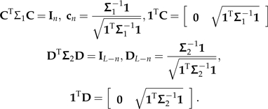I now show how C and D can be combined to yield a contrast decomposition of Σ. Let

where C ^{− n} and D ^{− (L − n)} denote the matrices C and D respectively after their final columns have been removed. In other words, the columns of C ^{− n} and D ^{− (L − n)} are the usual vectors of independent contrasts. Additionally,

let

where

and

are defined to be consistent with their introduction in the base case.

I suppress the algebra showing that M = P^TGH satisifies

That is to say, M is a contrast decomposition of Σ that has been constructed from the decompositions of the subtrees Σ₁ and Σ₂. This observation both completes the proof of the theorem and reveals a useful fact that is exploited throughout the manuscript. Disregarding the permutation matrix, the product GH has the block structure shown below:

The first n − 1 columns of GH, and hence n − 1 of the contrast vectors of Σ, are simply contrast vectors of Σ₁ with zeros appended to them. Moreover, another L − n − 1 columns of GH are simply contrast vectors of Σ₂ with zeros appended to them. This is completely intuitive; Felsenstein's independent contrasts are built from the bottom up, and here I am considering a tree (with PCM Σ) in terms of 2 subtrees (with PCMs Σ₁ and Σ₂) that are its immediate descendants. Only the final contrast constructed by Felsenstein's algorithm spans these 2 subtrees, and it is this contrast that is represented by the second column of the block representation of GH above. The phylogenetic perturbation results presented in the main text are achieved by isolating the effect of the change to this one vector.

References

- Abouheif E. Random trees and the comparative method: a cautionary tale. Evolution. 1998;52:1197–1204. doi: 10.1111/j.1558-5646.1998.tb01845.x. [DOI] [PubMed] [Google Scholar]
- Abouheif E. A method for testing the assumption of phylogenetic independence in comparative data. Evol. Ecol. Res. 1999;1:895–909. [Google Scholar]
- Butler MA, Schoener TW, Losos JB. The relationship between sexual size dimorphism and habitat use in Greater Antillean Anolis lizards. Evolution. 2000;54:259–272. [PubMed] [Google Scholar]
- Cavalli-Sforza LL, Edwards AW. Phylogenetic analysis: models and estimation procedures. Am. J. Hum. Genet. 1967;19:233–257. [PMC free article] [PubMed] [Google Scholar]
- Cavalli-Sforza LL, Piazza A. Analysis of evolution: evolutionary rates, independence and treeness. Theor. Popul. Biol. 1975;8:127–165. doi: 10.1016/0040-5809(75)90029-5. [DOI] [PubMed] [Google Scholar]
- Collar DC, O'Meara BC, Wainwright PC, Near TJ. Piscivory limits diversification of feeding morphology in centrarchid fishes. Evolution. 2009;63:1557–1573. doi: 10.1111/j.1558-5646.2009.00626.x. [DOI] [PubMed] [Google Scholar]
- Diaz-Uriarte R, Garland T. Testing hypotheses of correlated evolution using phylogenetically independent contrasts: sensitivity to deviations from Brownian motion. Syst. Biol. 1996;45:27–47. [Google Scholar]
- Diaz-Uriarte R, Garland T. Effects of branch length errors on the performance of phylogenetically independent contrasts. Syst. Biol. 1998;47:654–672. doi: 10.1080/106351598260653. [DOI] [PubMed] [Google Scholar]
- Felsenstein J. Maximum-likelihood estimation of evolutionary trees from continuous characters. Am. J. Hum. Genet. 1973;25:471–492. [PMC free article] [PubMed] [Google Scholar]
- Felsenstein J. The number of evolutionary trees. Syst. Zool. 1978;27:27–33. [Google Scholar]
- Felsenstein J. Phylogenies and the comparative method. Am. Nat. 1985;125:1–15. [Google Scholar]
- Felsenstein J. Phylogenies from molecular sequences: inference and reliability. Annu. Rev. Genet. 1988;22:521–565. doi: 10.1146/annurev.ge.22.120188.002513. [DOI] [PubMed] [Google Scholar]
- Felsenstein J. Sunderland (MA): Sinauer; 2004. Inferring phylogenies. [Google Scholar]
- Fisher DO, Owens IP. The comparative method in conservation biology. Trends Ecol. Evol. 2004;19:391–398. doi: 10.1016/j.tree.2004.05.004. [DOI] [PubMed] [Google Scholar]
- Garland T, Jr., Diaz-Uriarte R. Polytomies and phylogenetically independent contrasts: examination of the bounded degrees of freedom approach. Syst. Biol. 1999;48:547–558. doi: 10.1080/106351599260139. [DOI] [PubMed] [Google Scholar]
- Garland T, Ives AR. Using the past to predict the present: confidence intervals for regression equations in phylogenetic comparative methods. Am. Nat. 2000;155:346–364. doi: 10.1086/303327. [DOI] [PubMed] [Google Scholar]
- Grafen A. The phylogenetic regression. Philos. Trans. R. Soc. Lond. B. Biol Sci. 1989;326:119–157. doi: 10.1098/rstb.1989.0106. [DOI] [PubMed] [Google Scholar]
- Grafen A. The uniqueness of the phylogenetic regression. J. Theor. Biol. 1992;156:405–423. [Google Scholar]
- Guo H, Weiss RE, Gu X, Suchard MA. Time squared: repeated measures on phylogenies. Mol. Biol. Evol. 2007;24:352–362. doi: 10.1093/molbev/msl165. [DOI] [PubMed] [Google Scholar]
- Hansen TF, Martins EP. Translating between microevolutionary process and macroevolutionary patterns: the correlation structure of interspecific data. Evolution. 1996;50:1404–1417. doi: 10.1111/j.1558-5646.1996.tb03914.x. [DOI] [PubMed] [Google Scholar]
- Harvey PH, Pagel MD. The comparative method in evolutionary biology. Oxford: Oxford University Press; 1991. [Google Scholar]
- Huelsenbeck JP, Rannala B. Detecting correlations between characters in a comparative analysis with uncertain phylogeny. Evolution. 2003;57:1237–1247. doi: 10.1111/j.0014-3820.2003.tb00332.x. [DOI] [PubMed] [Google Scholar]
- Lass R. Historical lingusitics and language change. New York: Cambridge University Press; 1997. [Google Scholar]
- Legendre P, Desdevises Y. Independent contrasts and regression through the origin. J. Theor. Biol. 2009;259:727–743. doi: 10.1016/j.jtbi.2009.04.022. [DOI] [PubMed] [Google Scholar]
- Losos JB. An approach to the analysis of comparative data when a phylogeny is unavailable or incomplete. Syst. Biol. 1994;48:117–123. [Google Scholar]
- Lynch M. Methods for the analysis of comparative data in evolutionary biology. Evolution. 1991;45:1065–1080. doi: 10.1111/j.1558-5646.1991.tb04375.x. [DOI] [PubMed] [Google Scholar]
- Maddison WP. Reconstructing character evolution on polytomous cladograms. Cladistics. 1989;5:365–377. doi: 10.1111/j.1096-0031.1989.tb00569.x. [DOI] [PubMed] [Google Scholar]
- Martins EP. Conducting phylogenetic comparative studies when the phylogeny is not known. Evolution. 1996;50:12–22. doi: 10.1111/j.1558-5646.1996.tb04468.x. [DOI] [PubMed] [Google Scholar]
- Martins EP. Adaptation and the comparative method. Trends Ecol. Evol. 2000;15:296–299. doi: 10.1016/s0169-5347(00)01880-2. [DOI] [PubMed] [Google Scholar]
- Martins EP, Diniz-Filho JA, Housworth EA. Adaptive constraints and the phylogenetic comparative method: a computer simulation test. Evolution. 2002;56:1–13. [PubMed] [Google Scholar]
- Martins EP, Garland T. Phylogenetic analyses of the correlated evolution of continuous characters: a simulation study. Evolution. 1991;45:534–557. doi: 10.1111/j.1558-5646.1991.tb04328.x. [DOI] [PubMed] [Google Scholar]
- Martins EP, Hansen TF. Phylogenies and the comparative method: a general approach to incorporating phylogenetic information into the analysis of interspecific data. Am. Nat. 1997;149:646–667. [Google Scholar]
- Martins EP, Housworth EA. Phylogeny shape and the phylogenetic comparative method. Syst. Biol. 2002;51:873–880. doi: 10.1080/10635150290102573. [DOI] [PubMed] [Google Scholar]
- Mayr EW. Cambridge (MA): Harvard University Press; 1982. The growth of biological thought: diversity, evolution, and inheritance. [Google Scholar]
- Miles DB, Dunham AE. Comparative analyses of phylogenetic effects in the life-history patterns of iguanid reptiles. Am. Nat. 1992;139:848–869. [Google Scholar]
- Nunn CL, Barton RA. Comparative methods for studying primate adaptation and allometry. Evol. Anthropol. 2001;10:81–98. [Google Scholar]
- Oakley TH, Gu Z, Abouheif E, Patel NH, Li WH. Comparative methods for the analysis of gene-expression evolution: an example using yeast functional genomic data. Mol. Biol. Evol. 2005;22:40–50. doi: 10.1093/molbev/msh257. [DOI] [PubMed] [Google Scholar]
- Pagel M. Seeking the evolutionary regression coefficient—an analysis of what comparative methods measure. J. Theor. Biol. 1993;164:191–205. doi: 10.1006/jtbi.1993.1148. [DOI] [PubMed] [Google Scholar]
- Pagel M, Harvey PH. On solving the correct problem: wishing does not make it so. J. Theor. Biol. 1992;156:425–430. [Google Scholar]
- Purvis A, Garland T. Polytomies in comparative analyses of continuous characters. Syst. Biol. 1993;42:569–575. [Google Scholar]
- Purvis A, Gittleman JL, Luh HK. Truth or consequences—effects of phylogenetic accuracy on 2 comparative methods. J. Theor. Biol. 1994;167:293–300. [Google Scholar]
- Ridley M. The explanation of organic diversity: the comparative method and adaptations for mating. Oxford: Clarendon; 1983. [Google Scholar]
- Rohlf FJ. Comparative methods for the analysis of continuous variables: geometric interpretations. Evolution. 2001;55:2143–2160. doi: 10.1111/j.0014-3820.2001.tb00731.x. [DOI] [PubMed] [Google Scholar]
- Rohlf FJ. A comment on phylogenetic correction. Evolution. 2006;60:1509–1515. doi: 10.1554/05-550.1. [DOI] [PubMed] [Google Scholar]
- Sanford GM, Lutterschmidt WI, Hutchison VH. The comparative method revisited. Bioscience. 2002;52:830–836. [Google Scholar]
- Symonds MRE. The effects of topological inaccuracy in evolutionary trees on the phylogenetic comparative method of independent contrasts. Syst. Biol. 2002;51:541–553. doi: 10.1080/10635150290069977. [DOI] [PubMed] [Google Scholar]