Statistical Analysis of Fiber Bundles using Multi-tensor Tractography: Application to First-episode Schizophrenia

Abstract

This work proposes a new method to detect abnormalities in fiber bundles of first-episode (FE) schizophrenia patients. Existing methods have either examined a particular region of interest (ROI) or used voxel based morphometry (VBM) or used tracts generated using the single tensor model for locating statistically different fiber bundles. Further, a two-sample t-test, which assumes a Gaussian distribution for each population, is the most widely used statistical hypothesis testing algorithm.

In this study, we use the unscented Kalman filter based two-tensor tractography algorithm for tracing neural fiber bundles of the brain that connect 105 different cortical and subcortical regions. Next, fiber bundles with significant connectivity across the entire population were determined. Several diffusion measures derived from the two-tensor model were computed and used as features in the subsequent analysis. For each fiber bundle, an affine-invariant descriptor was computed, thus obviating the need for precise registration of patients to an atlas. A kernel based statistical hypothesis testing algorithm, that makes no assumption regarding the distribution of the underlying population, was then used to determine the abnormal diffusion properties of all fiber bundles for 20 FE patients and 20 age-matched healthy controls. Of the 1254 fiber bundles with significant connectivity, 740 fiber bundles were found to be significantly different in at least one diffusion measure after correcting for multiple comparisons. Thus, the changes affecting first-episode patients seem to be global in nature (spread throughout the brain).

1. Introduction

Both, post-mortem and neuroimaging studies have contributed significantly to what we know about the brain. MRI studies have demonstrated cortical volume reduction and ventricle enlargement in schizophrenia (Shenton et al., 2001; Cannon et al., 1998). This fact has been particularly informative in confirming early speculations that the brain is disordered in schizophrenia. There is also a growing body of evidence to suggest that a disturbance in connectivity between different brain regions, rather than abnormalities within the separate regions themselves, are responsible for at least some of the clinical symptoms and cognitive dysfunctions observed in schizophrenia (Davis et al., 2003; Kubicki et al., 2007). Thus, an interest in white matter fiber tracts is emerging, as these structures provide anatomical connections between distant, as well as proximal, brain regions. This interest coincides with the advent of Diffusion Tensor Imaging (DTI) and more recently High Angular Resolution Diffusion Imaging (HARDI), which makes it possible to evaluate the organization and coherence of white matter fiber tracts (Tuch et al., 2002).

Analyzing diffusion data using the single tensor model has been the most popular choice for investigating white matter abnormalities in a number of brain disorder studies. These studies are generally approached using one of three possible methods: (1) region-of-interest-(ROI) based methods, (2) voxel-based morphometry (VBM) methods and (3) fiber tract based methods. Many researchers have used ROI methods that are based on identifying anatomical brain regions and comparing the anisotropy or the extent of the region having high anisotropy (see Kubicki et al. (2007) and the references therein). Such studies assume prior knowledge about regions where the abnormalities are likely to occur. For studies where the anatomical ROI of potential abnormality is difficult to define precisely, voxel-based morphometry (VBM) methods tend to be used (Eriksson et al., 1998; Shenton et al., 2001; Rugg-Gunn et al., 2001; Price et al., 2007; Prez-Iglesias et al., 2010). A voxel-based strategy is more exploratory and is suitable for identifying unanticipated or unpredicted/unhypothesized areas of abnormal white matter morphology. However, the statistical differences obtained using such studies are heavily dependent on the registration (spatial normalization) algorithms being used. Further, VBM based methods examine each voxel separately, not all voxels jointly. This can result in biased interpretations of the data and it also overlooks interactions between different brain regions (Davatzikos, 2004).

Due to the aforementioned limitations of the above two methods, tract based analysis methods are fast becoming popular. Further, for diseases like schizophrenia, it is becoming increasingly evident that a disturbance in connection between different brain regions in addition to abnormalities within separate regions themselves, is responsible for the clinical symptoms and cognitive dysfunctions observed in this disorder. Thus, it is natural to analyze and locate abnormalities along fiber bundles using tract based methods.

Existing tract based methods require exact correspondence between the fiber bundles of all subjects. One approach taken by researchers (O’Donnell et al., 2007; Maddah et al., 2008) is to register the fractional anisotropy (FA) images to a template image in the atlas space to obtain an affine transformation or a diffeomorphic mapping. Tractography is performed in the subject space and the tracts are then mapped to the atlas space to obtain a correspondence between the fiber bundles. The fibers are then parameterized by arc-length and at each unit interval along the fiber, a t-test is used to find statistical difference between two groups (Maddah et al., 2008). Alternatively, the authors in (Goodlett et al., 2008) create an atlas and perform tractography in the atlas space. Fiber tracts are parameterized by B-splines and Hotelling’s T²-statistic is used to locate abnormalities.

In this paper, we will investigate abnormal fiber bundles in first-episode schizophrenia patients. This population set is typically younger and changes occurring at disease onset can be quite useful not only understanding the anatomical abnormalities, but also in analyzing risk for prodromal (high-risk) subjects. Further, since FE patients are not on medication for long time periods (unlike chronic patients), the impact of these medications on the brain anatomy is limited (compared to chronic subjects).

2. Our contributions

In this work, we propose to apply several new techniques to the study of first-episode schizophrenia. To date, most studies have used the single tensor model for analysis, despite it being a poor fit in regions of crossings and branchings (Tuch et al., 2002). In this study, for the first time, we will use fiber tracts generated using an unscented Kalman filter based two-tensor tractography algorithm(Malcolm et al., 2009a). This method allows for recovering tracts that pass through branching and crossing regions of the brain (Malcolm et al., 2010).

Statistical analysis to detect group differences has been primarily done using the standard t-test or the Hotelling’s T²-statistic (both assume a Gaussian distribution for the two sample sets). In this work, we propose to use the non-parametric hypothesis testing algorithm of (Gretton et al., 2008), which we will refer to as the kernel hypothesis algorithm, to find fiber bundles that are statistically different between first-episode (FE) patients and matched normal controls (NC). This algorithm tests the null hypothesis that the two populations have same probability distribution, without any assumption on the type (say, Gaussian) of distribution.

Further, most of the existing literature has focused on analyzing a selected set of fiber bundles for detecting abnormalities. In this paper, we perform a connectome-like analysis by testing for group differences between fiber bundles connecting 105 gray and white matter regions of the brain. Thus, this is a first study that will examine fiber bundles of the entire brain extracted using multi-fiber model with group differences being computed using a kernel based hypothesis testing algorithm. In addition, application of this method to first-episode schizophrenia is also novel.

3. Preliminaries

In this section, we provide a brief background on the two-tensor tractography algorithm (Malcolm et al., 2009a,b, 2010), as well as the kernel based non-parametric hypothesis testing algorithm (Gretton et al., 2008).

3.1. Unscented Kalman Filter based tractography

Recently, we proposed a method for simultaneous fiber model estimation and tractography using the unscented Kalman filter (UKF) (Malcolm et al., 2009a). Other approaches to tractography estimate the local fiber orientation at each voxel independently and thus do not take into account the correlation in diffusion of water along the fiber path. In the UKF based method, fiber tracking is formulated as recursive estimation: at each step of tracing the fiber, the current estimate is guided by the previous. Thus, correlation in diffusion and spatial regularization is incorporated as part of the model estimation step.

In this work, the signal is modeled as a mixture of two tensors and tractography is performed within a filtering framework. Starting from a seed point, each fiber is traced to its termination using an unscented Kalman filter to simultaneously fit the local model and propagate in the most consistent direction. Despite the presence of noise and uncertainty, this provides a robust estimate of the local structure at each point along the fiber.

Mathematically, the signal model for two equally weighted tensors is given by:

$$S({\mathbf{u}}_i)=\frac{S_0}{2}(\exp \{-b{\mathbf{u}}_i^T{D}_1{\mathbf{u}}_i\}+\exp \{-b{\mathbf{u}}_i^T{D}_2{\mathbf{u}}_i\}),$$ (1)

where D₁, D₂ are the two diffusion tensors, b is the b-value, S(u_i) is the measured signal in gradient direction u_i and S₀ is the baseline signal obtained using zero diffusion sensitizing gradient. In this work, we assume the diffusion tensor to be cigar-shaped by enforcing the two minor eigenvalues to be equal. Thus, we use the following parameterization of the diffusion tensor:

$$D={\mathrm{\lambda }}_1{\mathbf{mm}}^T+{\mathrm{\lambda }}_2({\mathbf{pp}}^T+{\mathbf{qq}}^T),$$ (2)

where m is the principal diffusion direction, λ₁ > λ₂ are the two eigenvalues, and p, q are the remaining eigenvector’s of D. As shown in (Malcolm et al., 2009a), the free parameters for each diffusion tensor are [m λ₁ λ₂], which are recursively estimated using the unscented Kalman filter.

Several diffusion measures such as, fractional anisotropy (FA), axial diffusivity, perpendicular diffusivity, relative anisotropy, trace, etc. are used by the neuroscience community. However, a set of three orthogonal diffusion measures were proposed in (Kindlmann et al., 2007), which capture all aspects of the shape of a diffusion tensor. These measures are FA, norm (N) and mode (M) of the tensor defined below:

$$\mathrm{N}=\parallel D\parallel ,\mathrm{FA}=\frac{\sqrt{3}\stackrel{\sim }{D}}{\sqrt{2}\parallel D\parallel },\mathrm{M}=3\sqrt{6}\mid \left(\frac{\stackrel{\sim }{D}}{\parallel \stackrel{\sim }{D}\parallel }\right)\mid ,\stackrel{\sim }{D}=D-\frac{1}{3}\mathit{tr}(D)I$$

where, |.| denotes the determinant, tr(.) is the trace, I is the identity matrix and ∥.∥ denotes the frobenius norm of a matrix. These measures can be computed for each tensor, and thus six features are obtained.

3.2. Kernel Hypothesis Testing

Most of the statistical studies done by the neuroscience community is using the standard t-test or some variants of it. This test assumes that the distribution of samples from the two population is Gaussian and test’s the hypothesis that their mean’s are equal. Assumption of Gaussianity may be a limitation in several cases. While there are nonparametric methods, such as the Kolmogorov-Smirnov, that make no assumption about the distribution of the population, the kernel based hypothesis testing algorithm of Gretton et al. (2008) has been shown to have better performance than most of the existing algorithms on several data sets.

As such, we will use the kernel based method of Gretton et al. (2008) for statistical hypothesis testing. This method has several advantages, chief among them are : a) It can be used with high dimensional data without sacrificing robustness and accuracy. b) The data need not necessarily lie in a Euclidean vector space, i.e., any type of data with an appropriate kernel can be used. c) This method computes statistical differences without any assumption on the distribution from which the samples are drawn. Thus, subtle differences can be captured using the kernel based method.

This method tests the hypothesis of two distributions (p, q) being equal p = q. The test statistic used is the maximum mean discrepancy (MMD) between the two samples. Let F be a class of functions f : X → ℝ and p, q be probability distributions (with domain X), then MMD is defined as: MMD[F, p, q ] = sup_f∈F (E_x~p[f(x)] − E_y~q [f(y)]), where E represents the expected value. To put it simply, MMD is the maximum difference between the mean of the two sample populations as computed over all possible functions f ∈ F.

Computing MMD involves, mapping the data to a reproducing kernel Hilbert space (RKHS) and computing the inner product (between high dimensional features) in this space using an appropriate kernel (Gaussian in our case). If MMD is greater than a certain threshold, the null hypothesis (p = q) is rejected. The hypothesis threshold is selected based on significance level α, typically set to 0.05. We should point out an important difference while inferring results from this test: The null hypothesis is rejected if MMD is greater than a threshold. Thus, higher the MMD, greater is the statistical significance. This is in contrast to the interpretation of p-value (for t-test), where lower p-value indicates higher statistical difference.

4. Methods

The block diagram shown in Figure 1 gives the steps involved in the statistical analysis of fiber bundles. Details about each step are given in the following subsections.

Figure 1.

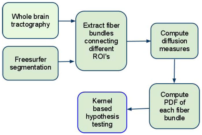
Block diagram indicating the steps involved in the statistical analysis of fiber bundles

4.1. Whole brain tractography

The UKF based two-tensor tractography algorithm of (Malcolm et al., 2009a) was used to trace fiber paths. Seeding was done in all the voxels where single tensor FA was greater than 0.18. Each voxel was seeded 10 times (randomly), and each fiber was traced from seed to termination, with the termination criteria being FA < 0:15, for the primary tensor component (the component most consistent with the tracking direction) being followed.

4.2. FreeSurfer segmentation

One way to obtain correspondence between fiber bundles across subjects, is to reliably segment the brain into different anatomical regions. We achieved this, by using the Freesurfer software (surfer.nmr.mgh.harvard.edu) to segment T1-weighted SPGR image of each subject into 180 different cortical and subcortical gray and white matter regions. A T2 image (which was in the same coordinate space as the SPGR image) was then diffeomorphically registered to the baseline (S₀) diffusion weighted image of the same subject using the FNIRT algorithm of the FSL software (Smith et al., 2004). This diffeomorphism was applied to the label map (180 labels) obtained from T1 segmentation to obtain a label map in the coordinate space of the diffusion images. Thus, a correspondence was obtained across subjects by representing each region with the same label.

4.3. Fiber bundle extraction

Once anatomical correspondence was achieved, fibers connecting any two regions-of-interest (ROI) were extracted. In order to ensure that the connections are distinct and the fiber bundles do not overlap, only those fibers that have their end-points in the desired ROI’s were retained. Further, cortical gray and white matter regions from the Freesurfer segmentation were merged to obtain 105 unique ROI’s. Fiber bundle extraction was done for each subject, and a connectivity matrix (105 × 105) was computed for each subject. In order to remove spurious connections due to noise as well as to obtain robust statistics on the data, any connection with less than 10 fibers was marked as “not connected” in the connectivity matrix. Finally, a set of 1254 fiber bundles (connections) which were consistent across all 40 subjects were retained for further analysis.

4.4. Compute diffusion measures

Several diffusion measures have been used by the neuroscience community. However, a set of three orthogonal diffusion measures that capture all aspects of the shape of a diffusion tensor were proposed by (Kindlmann et al., 2007). These measures, as defined in section 3.1, will be used in our analysis. In particular, each of the six measures, namely, FA (fractional anisotropy), M (mode) and N (norm) were computed at each point along the fiber tract for all fiber bundles.

4.5. Estimate probability distribution

For each diffusion measure of a fiber bundle, a nonparametric probability distribution function (PDF) was computed. This forms an affine-invariant representation of the fiber bundle and is robust to misalignment. Further, all the statistical information regarding each fiber bundle as given by the three diffusion measures is captured by the PDF. We should note that, we use only those diffusion measures that correspond to the tensor component along the fiber path, since we are only interested in abnormalities along the path and not across the path. Thus, for each subject, we have a representation denoted by $P={\left\{{\left[p_{\mathit{fa}}{p}_m{p}_n\right]}_i\right\}}_{i=1}^{1254}$, where p_fa, p_m, p_n are the PDF’s of the FA, mode and norm respectively for each fiber bundle i. The PDF’s were computed with 300 bins, making each PDF a vector of dimension 300 × 1.

4.6. Kernel hypothesis testing

For each fiber bundle, the kernel based statistical hypothesis testing algorithm of (Gretton et al., 2008), as described earlier, was used to determine statistical differences between the two groups (FE and NC). For each diffusion measure, say FA, p_fa was used as a feature for which statistical differences were investigated. This is in contrast to traditional strategies where the average FA is used to find differences. Since we use the entire probability distribution (as opposed to the first moment only), all the statistical information about the fiber bundle is used in the analysis. All three diffusion measures for each of the 1254 fiber bundles were investigated for statistical differences. To correct for multiple comparisons, a false discovery rate (FDR) of 0.05 was used.

Statistical difference in the context of the kernel based method is considered significant, if MMD > t, where t is a threshold determined by the parameter β, typically set to 0.05. Further, higher the value of MMD, the greater is the difference. In the remainder of this discussion, we will often use the value D_k = MMD − t, which indicates the level of significance. Further, to correct for multiple comparisons, we computed D_k for each fiber bundle and each diffusion measure. Correction for multiple comparison was done in the following manner:

Let $D_k^{(1)},\dots D_k^{(m)}$ be the m independent tests with decreasing significance level, i.e., $D_k^{(1)}>D_k^{(2)}>\dots D_k^{(m)}$. For a given significance level α, find the largest x such that $D_k^{(x)}\ge \frac{x}{m}\alpha$. Then, all tests with i = 1 to x are accepted as statistically significant hypotheses. The FDR is computed using the expression $\mathrm{FDR}=\frac{\alpha (m+1)}{2m}$. In this work, we set α = 0.10.

5. Patient population

The study consisted of 20 first-episode patients and 20 age-matched normal controls. Figure 2 provides the demographic and clinical details of all subjects. Exclusion criteria for all subjects included any history of neurological disorders, electroconvulsive shock treatment, drub abuse or alcoholism. Schizophrenia diagnosis was determined by DSM-IV criteria using the Structured Clinical Interview for DSM-IV. Patient recruitment was done as part of the Boston CIDAR Center (www.bostoncidar.org).

Figure 2.

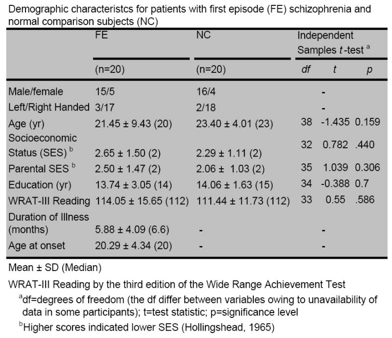
Demographics of the subjects in the study.

6. Data acquisition

Diffusion Weighted images (DWI) scans were acquired on a 3 Tesla GE system using an echo planar imaging (EPI) DWI sequence. A double echo option was used to reduce eddy-current related distortions. To reduce impact of EPI spatial distortion, an 8 Channel coil was used to allow to perform parallel imaging using ASSET (Array Spatial Sensitivity Encoding Techniques, GE) with a SENSE-factor (speed-up) of 2. Acquisitions have 51 gradient directions with b=900 and 8 baseline scans with b=0. The original GE sequence was modified to increase spatial resolution, and to further minimize image artifacts. The following scan parameters were used: TR 17000 ms, TE 78 ms, FOV 24 cm, 144×144 encoding steps, 1.7 mm slice thickness. All scans had 85 axial slices parallel to the AC-PC line covering the whole brain.

The data was pre-processed to reduce the effects of noise (Aja-Fernandez et al., 2008). To remove artifacts due to eddy currents and head motion, an affine registration (using FLIRT) of the diffusion weighted images to the baseline image was done for each subject.

7. Results

Of the 1254 fiber bundles that were investigated, 740 fiber bundles were found to be statistically different in atleast one diffusion measure. Figure 3 shows a network graph of the connections that were found to be statistically different. Statistical significance decreases from green to red. Figure 4 shows volumetric rendering of the significance level of different regions in the brain. Bright red indicates higher statistical difference. The volume was computed by associating the significance value D_k with each voxel through which a fiber bundle passed. Figures 5 and 6 shows several coronal and sagittal slices from this volume with statistical significance overlaid on the FA images. From these figures, it becomes clear that the cerebellum region is highly abnormal in FE patients. It is important to note that, the views do not show “exact” location of abnormalities but only the fiber paths that are abnormal. Figure 8 shows the significantly different connections with statistical significance increasing from blue to red. The table in appendix gives a list of all the 98 ROIs that are used in forming the anatomical network. Naming convention is the same as in Freesurfer software.

Figure 3.

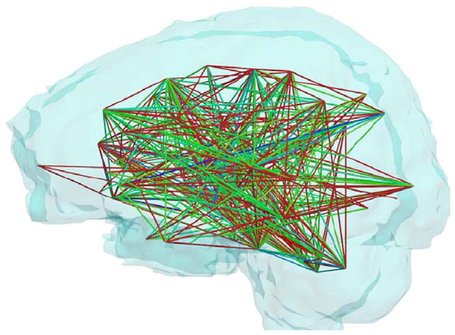
Graphical representation of the connections that were found to be statistically different in FE patients. Statistical significance decreases from green to blue to red.

Figure 4.

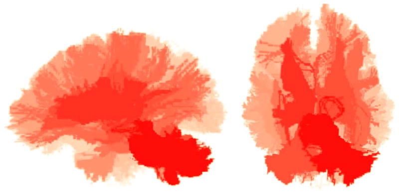
Two views of the volumetric rendering of statistical differences with increasing red intensity indicating higher difference.

Figure 5.

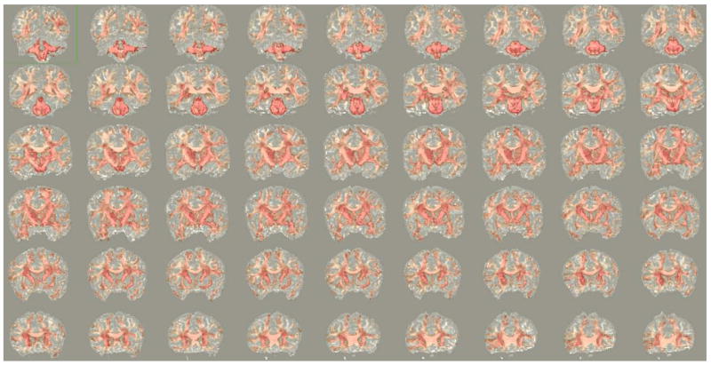
Coronal slices showing statistical differences (overlaid on FA images), with significance decreasing from red to white.

Figure 6.

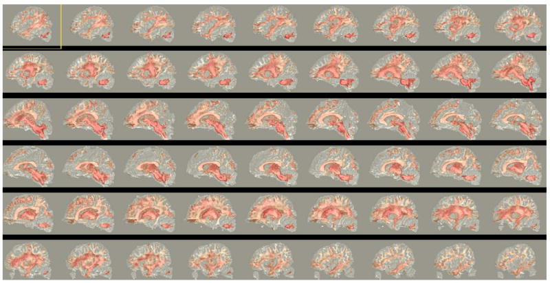
Sagittal slices showing statistical differences (overlaid on FA images), with significance decreasing from red to white.

Figure 8.

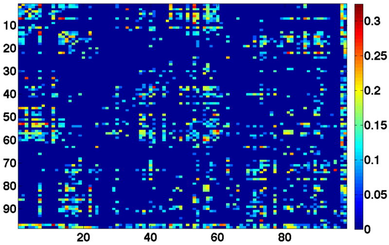
Matrix showing the statistically different connections for FE patients. Significance increases from blue (no connection) to red.

Given that a significant number of fiber bundles were found to be different, the abnormalities in FE patients seems to be global in nature rather being localized to any specific bundle or region. Consequently, we performed statistical analysis of global features derived from the two-tensor model. First, a non-parametric probability distribution was computed for each of the six diffusion measures (FA, M, N for each tensor). This forms an transformation-invariant representation since the probability distribution is independent of any co-ordinate system. This representation allows for doing away with the need for registration of the subjects. Next, the kernel based hypothesis testing algorithm was used to find statistical differences between the two populations, with the PDF being the feature vector. While no difference were reported for FA or mode, the norm of each tensor (N₁, N₂), showed significant difference with D_k = 0.27 and D_k = 0.26 respectively for both the norms. Figure 7 shows PDF’s for four features (FA₁, N₁, FA₂, N₂) for all subjects. As seen in figure 7 as well as from the list of fiber bundles in the appendix, mean diffusivity (which is proportional to norm of the tensor) of each tensor is higher in FE patients even at the global level. This observation is also consistent with recently published work of (Narr et al., 2009).

Figure 7.

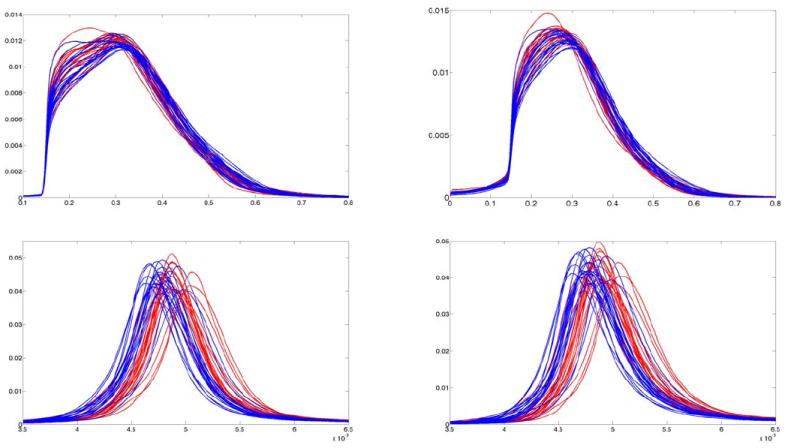
Top: Probability distribution functions of FA (FA1 and FA2) for 20 FE (red) and 20 NC (blue) subjects. Bottom: PDF’s of norm (N) of each of the tensor components for 20 FE (red) and 20 NC (blue) subjects.

8. Conclusion

In this work, we applied several new techniques for detecting abnormalities in first-episode schizophrenia patients. In particular, we used a multi-tensor tractography algorithm to trace fiber tracts that pass through crossing regions to connect 105 different gray and white matter regions of the brain. A kernel based non-parametric statistical hypothesis algorithm was then used to detect abnormal fiber bundles of FE patients. It was noticed that a significant number of fiber bundles were statistically different, which consequently showed in the global analysis of diffusion features. In particular, norm (proportional to mean diffusivity) of the two tensors was higher in FE patients than in normal controls.

Appendix A. Freesurfer ROI’s shown in Figure 5

Table A.1.

Freesurfer label names and numbers

Serial Number	Label name	Label number
1	Left-Cerebellum-White-Matter	7
2	Left-Cerebellum-Cortex	8
3	Left-Thalamus-Proper	10
4	Left-Caudate	11
5	Left-Putamen	12
6	Left-Pallidum	13
7	Brain-Stem	16
8	Left-Hippocampus	17
9	Left-Amygdala	18
10	Left-Accumbens-area	26
11	Left-VentralDC	28
12	Left-choroid-plexus	31
13	Right-Cerebellum-White-Matter	46
14	Right-Cerebellum-Cortex	47
15	Right-Thalamus-Proper	49
16	Right-Caudate	50
17	Right-Putamen	51
18	Right-Pallidum	52
19	Right-Hippocampus	53
20	Right-Amygdala	54
21	Right-Accumbens-area	58
22	Right-VentralDC	60
23	Right-vessel	62
24	Right-choroid-plexus	63
25	unknown	251
26	unknown	252
27	unknown	253
28	unknown	254
29	unknown	255
30	ctx-lh-unknown	1000
31	ctx-lh-bankssts	1001
32	ctx-lh-caudalanteriorcingulate	1002
33	ctx-lh-caudalmiddlefrontal	1003
34	ctx-lh-cuneus	1005
35	ctx-lh-entorhinal	1006
36	ctx-lh-fusiform	1007
37	ctx-lh-inferiorparietal	1008
38	ctx-lh-inferiortemporal	1009
39	ctx-lh-isthmuscingulate	1010
40	ctx-lh-lateraloccipital	1011
41	ctx-lh-lateralorbitofrontal	1012
42	ctx-lh-lingual	1013
43	ctx-lh-medialorbitofrontal	1014
44	ctx-lh-middletemporal	1015
45	ctx-lh-parahippocampal	1016
46	ctx-lh-paracentral	1017
47	ctx-lh-parsopercularis	1018
48	ctx-lh-parsorbitalis	1019
49	ctx-lh-parstriangularis	1020
50	ctx-lh-pericalcarine	1021
51	ctx-lh-postcentral	1022
52	ctx-lh-posteriorcingulate	1023
53	ctx-lh-precentral	1024
54	ctx-lh-precuneus	1025
55	ctx-lh-rostralanteriorcingulate	1026
56	ctx-lh-rostralmiddlefrontal	1027
57	ctx-lh-superiorfrontal	1028
58	ctx-lh-superiorparietal	1029
59	ctx-lh-superiortemporal	1030
60	ctx-lh-supramarginal	1031
61	ctx-lh-temporalpole	1033
62	ctx-lh-transversetemporal	1034
63	ctx-rh-unknown	2000
64	ctx-rh-bankssts	2001
65	ctx-rh-caudalanteriorcingulate	2002
66	ctx-rh-caudalmiddlefrontal	2003
67	ctx-rh-cuneus	2005
68	ctx-rh-entorhinal	2006
69	ctx-rh-fusiform	2007
70	ctx-rh-inferiorparietal	2008
71	ctx-rh-inferiortemporal	2009
72	ctx-rh-isthmuscingulate	2010
73	ctx-rh-lateraloccipital	2011
74	ctx-rh-lateralorbitofrontal	2012
75	ctx-rh-lingual	2013
76	ctx-rh-medialorbitofrontal	2014
77	ctx-rh-middletemporal	2015
78	ctx-rh-parahippocampal	2016
79	ctx-rh-paracentral	2017
80	ctx-rh-parsopercularis	2018
81	ctx-rh-parsorbitalis	2019
82	ctx-rh-parstriangularis	2020
83	ctx-rh-pericalcarine	2021
84	ctx-rh-postcentral	2022
85	ctx-rh-posteriorcingulate	2023
86	ctx-rh-precentral	2024
87	ctx-rh-precuneus	2025
88	ctx-rh-rostralanteriorcingulate	2026
89	ctx-rh-rostralmiddlefrontal	2027
90	ctx-rh-superiorfrontal	2028
91	ctx-rh-superiorparietal	2029
92	ctx-rh-superiortemporal	2030
93	ctx-rh-supramarginal	2031
94	ctx-rh-frontalpole	2032
95	ctx-rh-temporalpole	2033
96	ctx-rh-transversetemporal	2034
97	wm-lh-centrum-semiovale	5001
98	wm-rh-centrum-semiovale	5002

References

- Aja-Fernandez S, Niethammer M, Kubicki M, Shenton M, Westin C. Restoration of dwi data using a rician lmmse estimator. IEEE transactions on medical imaging. 2008;27(10):1389–1403. doi: 10.1109/TMI.2008.920609. [DOI] [PMC free article] [PubMed] [Google Scholar]
- Cannon T, van Erp T, Huttunen M, Lonnqvist J, Salonen O, Valanne L, Poutanen V, Standertskjold-Nordenstam C, Gur R, Yan M. Regional gray matter, white matter, and cerebrospinal fluid distributions in schizophrenic patients, their siblings, and controls. Archives of General Psychiatry. 1998;55(12):1084. doi: 10.1001/archpsyc.55.12.1084. [DOI] [PubMed] [Google Scholar]
- Davatzikos C. Why voxel-based morphometric analysis should be used with great caution when characterizing group differences. Neuroimage. 2004;23(1):17–20. doi: 10.1016/j.neuroimage.2004.05.010. [DOI] [PubMed] [Google Scholar]
- Davis K, Stewart D, Friedman J, Buchsbaum M, Harvey P, Hof P, Buxbaum J, Haroutunian V. White matter changes in schizophrenia: evidence for myelin-related dysfunction. Archives of General Psychiatry. 2003;60(5):443–457. doi: 10.1001/archpsyc.60.5.443. [DOI] [PubMed] [Google Scholar]
- Eriksson P, Perfilieva E, Björk-Eriksson T, Alborn A, Nordborg C, Peterson D, Gage F. Neurogenesis in the adult human hippocampus. Nature medicine. 1998;4(11):1313–1317. doi: 10.1038/3305. [DOI] [PubMed] [Google Scholar]
- Goodlett C, Fletcher P, Gilmore J, Gerig G. Group statistics of DTI fiber bundles using spatial functions of tensor measures. MICCAI. 2008:1068–1075. doi: 10.1007/978-3-540-85988-8_127. [DOI] [PMC free article] [PubMed] [Google Scholar]
- Gretton A, Borgwardt K, Rasch M, Scholkopf B, Smola A. A kernel method for the two-sample-problem. Journal of Machine Learning Research. 2008;1:1–10. [Google Scholar]
- Kindlmann G, Ennis D, Whitaker R, Westin C. Diffusion tensor analysis with invariant gradients and rotation tangents. TMI. 2007;26(11):1483–1499. doi: 10.1109/TMI.2007.907277. [DOI] [PubMed] [Google Scholar]
- Kubicki M, McCarley R, Westin C-F, Park H-J, Maier S, Kikinis R, Jolesz F, Shenton M. A review of diffusion tensor imaging studies in schizophrenia. J of Psychiatric Research. 2007;41:15–30. doi: 10.1016/j.jpsychires.2005.05.005. [DOI] [PMC free article] [PubMed] [Google Scholar]
- Maddah M, Kubicki M, Wells W, Westin C-F, Shenton M, Grimson W. Findings in schizophrenia by tract-oriented DT-MRI analysis. MICCAI. 2008 doi: 10.1007/978-3-540-85988-8_109. [DOI] [PMC free article] [PubMed] [Google Scholar]
- Malcolm J, Shenton M, Rathi Y. Neural tractography using an unscented Kalman filter. IPMI. 2009a:126–138. doi: 10.1007/978-3-642-02498-6_11. [DOI] [PMC free article] [PubMed] [Google Scholar]
- Malcolm JG, Michailovich O, Bouix S, Westin C-F, Shenton ME, Rathi Y. A filtered approach to neural tractography using the Watson directional function. Medical Image Analysis. 2010;14:58–69. doi: 10.1016/j.media.2009.10.003. [DOI] [PMC free article] [PubMed] [Google Scholar]
- Malcolm JG, Shenton ME, Rathi Y. Two-tensor tractography using a constrained filter. Medical Image Computing and Computer Assisted Intervention (MICCAI) 2009b:894–902. doi: 10.1007/978-3-642-04268-3_110. [DOI] [PMC free article] [PubMed] [Google Scholar]
- Narr K, Hageman N, Woods R, Hamilton L, Clark K, Phillips O, Shattuck D, Asarnow R, Toga A, Nuechterlein K. Mean diffusivity: A biomarker for CSF-related disease and genetic liability effects in schizophrenia. Psychiatry research. 2009;171(1):20. doi: 10.1016/j.pscychresns.2008.03.008. [DOI] [PMC free article] [PubMed] [Google Scholar]
- O’Donnell L, Westin C-F, Golby A. Tract-based morphometry. MICCAI. 2007:161–168. [PubMed] [Google Scholar]
- Prez-Iglesias R, Tordesillas-Gutirrez D, Barker GJ, McGuire PK, Roiz-Santiaez R, Mata I, de Lucas EM, Quintana F, Vazquez-Barquero JL, Crespo-Facorro B. White matter defects in first episode psychosis patients: A voxelwise analysis of diffusion tensor imaging. NeuroImage. 2010;49(1):199–204. doi: 10.1016/j.neuroimage.2009.07.016. [DOI] [PubMed] [Google Scholar]
- Price G, Cercignani M, Parker GJ, Altmann DR, Barnes TR, Barker GJ, Joyce EM, Ron MA. Abnormal brain connectivity in first-episode psychosis: A diffusion mri tractography study of the corpus callosum. NeuroImage. 2007;35(2):458–466. doi: 10.1016/j.neuroimage.2006.12.019. [DOI] [PMC free article] [PubMed] [Google Scholar]
- Rugg-Gunn F, Eriksson S, Symms M, Barker G, Duncan J. Diffusion tensor imaging of cryptogenic and acquired partial epilepsies. Brain. 2001;124(3):627. doi: 10.1093/brain/124.3.627. [DOI] [PubMed] [Google Scholar]
- Shenton M, Dickey C, Frumin M, McCarley R. A review of MRI findings in schizophrenia. Schizophrenia Research. 2001;49(1-2):1–52. doi: 10.1016/s0920-9964(01)00163-3. [DOI] [PMC free article] [PubMed] [Google Scholar]
- Smith S, Jenkinson M, Woolrich M, Beckmann C, Behrens T, Johansen-Berg H, Bannister P, De Luca M, Drobnjak I, Flitney D, et al. Advances in functional and structural MR image analysis and implementation as FSL. Neuroimage. 2004;23:S208–S219. doi: 10.1016/j.neuroimage.2004.07.051. [DOI] [PubMed] [Google Scholar]
- Tuch D, Reese T, Wiegella M, Makris N, Belliveau J, Wedeen V. High angular resolution diffusion imaging reveals intravoxel white matter fiber heterogeneity. Magnetic Resonance in Medicine. 2002;48:577–582. doi: 10.1002/mrm.10268. [DOI] [PubMed] [Google Scholar]