An integrated computational approach to the analysis of NMR relaxation in proteins: application to ps-ns mainchain ¹⁵N-¹H and global dynamics of the Rho GTPase binding domain of plexin-B1

Abstract

An integrated computational methodology for interpreting NMR spin relaxation in proteins has been developed. It combines a two-body coupled-rotator stochastic model with a hydrodynamics-based approach for protein diffusion, together with molecular dynamics based calculations for the evaluation of the coupling potential of mean force. The method is applied to ¹⁵N relaxation of N–H bonds in the Rho GTPase binding (RBD) domain of plexin-B1, which exhibits intricate internal mobility. Bond vector dynamics are characterized by a rhombic local ordering tensor, S, with principal values $S_0^2\text{ and }{S}_2^2$, and an axial local diffusion tensor, D₂, with principal values D_2,‖ and D_2,⊥. For α-helices and β-sheets we find that $S_0^2~-0.5$ (strong local ordering), $-1.2<S_2^2<-0.8$ (large S tensor anisotropy), D_2,⊥ ~ D₁ = 1.93×10⁷ s⁻¹ (D₁ is the global diffusion rate), and log(D_2,‖ / D₁) ~ 4. For α-helices the z-axis of the local ordering frame is parallel to the C^α–C^α axis. For β-sheets the z-axes of the S and D₂ tensors are parallel to the N–H bond. For loops and terminal chain segments the local ordering is generally weaker and more isotropic. On average, D_2,⊥ ~ D₁ also, but log(D_2,‖ / D₁) is on the order of 1–2. The tensor orientations are diversified. This study sets forth an integrated computational approach for treating NMR relaxation in proteins by combining stochastic modeling and molecular dynamics. The approach developed provides new insights by its application to a protein that experiences complex dynamics.

1. Introduction

NMR emerged as a powerful method for investigating the structural and dynamic properties of bio-macromolecules, in particular proteins.^1–9 Three-dimensional solution structures are determined using ¹⁵N,¹³C–labeled, and in some cases also ²H-labeled proteins. Auto-correlated^1–4 and cross-correlated^{5 15}N relaxation of N–H bonds, and recently also ¹³C and ²H relaxation of additional probes,^6,7,8 are used to study backbone dynamics. ²H and ¹³C relaxation is used to study (side-chain) methyl dynamics.⁹ Information on dissipative properties (rotational reorientation of the protein and the probe), local restrictions at the site of the motion of the probe, and features of local geometry, can be obtained.^10–12 This kind of information is important when processes such as binding and reactivity, which are associated with the dynamics of the molecules involved, are studied.

In principle, structural and dynamic information at the atom level can be obtained using molecular dynamics (MD) simulations.^13–15 A number of difficulties are encountered, however. The information generated is very complex and the derivation of spectral density functions, which underlie the NMR relaxation rates, typically requires ad hoc assumptions. Software and hardware solutions for generating microsecond long trajectories are becoming available.¹⁶ However, even these trajectories are fraught with problems of inadequate sampling of the conformational space when the process of interest evolves on time scales of several tens of nanoseconds. To address this problem methodologies such as umbrella sampling,^17,18 metadynamics,^19,20 adaptive biasing force^21,22 and replica exchange^23,24 have been developed.

An effective approach in dealing with these matters is to identify a small number of essential (or relevant) coordinates that primarily influence the physical observables of interest (in this case, the NMR relaxation parameters), while the remaining coordinates affect the analysis in an average way. Stochastic methods belong to such an approach, where the “non-relevant” coordinates act as a thermal bath imposing fluctuation-dissipation on the relevant ones. The choice of the relevant coordinates can be guided by chemical insight in the case of small molecules;²⁵ however, for proteins this strategy is not practical. Several laboratories have explored the possibility of employing (when appropriate) relatively short MD trajectories to acquire information on the relevant coordinates. Techniques such as metadynamics and Markovian States Modeling have been used in this context.^26,27

Semi-phenomenological mesoscopic approaches have been introduced to overcome the complexity of describing protein dynamics. The traditional model-free (MF) approach belongs to this group,^28–30 as it is essentially a simple description of protein dynamics based on an approximate two-body framework. An analytical form of the measurable spectral density is obtained in the limit of statistical independence between the local motion of the probe and the global motion of the protein, and under the assumption of simple tensorial properties. A more precise description that can take into account the coupling between the local and global dynamics of the protein has been provided by the Slowly Relaxing Local Structure (SRLS) approach of Polimeno and Freed,^31–33 which has been applied to NMR spin relaxation in proteins.^34–37 This model associates the dynamics of the molecule with that of a Smoluchowski (coupled) two-body system with general tensorial properties. One body represents the overall tumbling of the protein, whereas the other body describes (collectively) the internal motions experienced by the probe.

SRLS has been applied extensively; new and interesting insights have emerged (e.g., Refs. ^38–43). However, its potential cannot be fully exploited because the experimental data sets are limited. For example, for ¹⁵N relaxation a typical data set comprises six points – ¹⁵N T₁, T₂ and ¹⁵N–{¹H} NOE acquired at two magnetic fields. On the other hand, the most recent fitting scheme for SRLS^42,43 allows for three principal components of the (rhombic) global diffusion tensor, three principal components of the (rhombic) local diffusion tensor, and the Euler angles that define their arbitrary orientations. It features a coupling potential that can include up to five terms, and a rhombic ordering tensor with arbitrary orientation and principal values defined in terms of the coupling potential. The principal axes frames of the local ordering and local diffusion tensors can be separated. Finally, the parameters that define the magnetic tensors also enter the analysis when the SRLS model is "interfaced" (geometrically) with the NMR component.

Clearly, one has to resort to simplifications in terms of tensor symmetry and local geometry. As typically^1–4,7 (although not always^5,6,8) assumed in MF, we have taken the magnetic tensors to be known and constant.^44–46 We have found that a minimum of four variables are required for appropriate description of local motions in proteins.³⁷ These are the rate of local motion, D₂, the coefficients $c_0^2\text{ and }{c}_2^2$ that define a rhombic coupling potential, and one angle, β_D, associated with the relative orientation of the local ordering frame and the major magnetic frame. Even with only four variables, the data fitting process has often led to relatively large uncertainties in the best-fit parameters. These uncertainties are related to the necessarily complex functional form of the measurable spectral density, combined with the paucity of the experimental data in the Redfield limit. In some cases, the computational cost of the analysis is high because long calculations are carried out repeatedly. Finally, problems inherent to nonlinear least squares solvers, associated in particular with calculations that get trapped in local minima, are encountered. The adverse implications of these issues are expected to be mitigated when some of the SRLS parameters are calculated separately and subsequently fixed in the data fitting process.

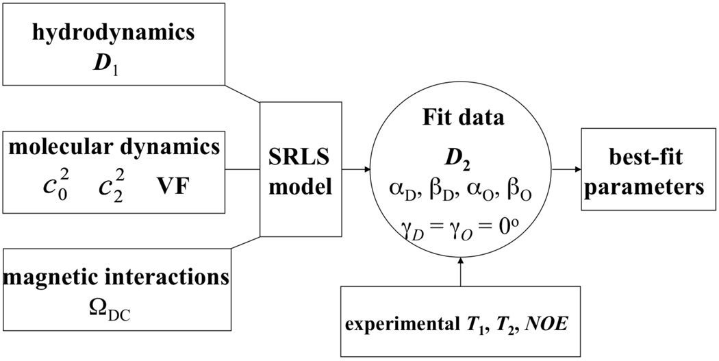
In this study we make a first attempt to develop such a methodology. Our integrated computational approach for the interpretation of NMR relaxation in proteins is centered on a stochastic model. Integrated approaches that combine stochastic models, quantum chemical methods, and hydrodynamics-based techniques, have been developed by some of us and applied successfully to ESR and NMR relaxation data of small molecules.^25,47,48 In these developments multi-component non linear fitting is either avoided, or reduced to a fitting scheme that features a small number of variables. The computational approach developed in this study comprises three components. (1) The global diffusion tensor, D₁, is calculated with a hydrodynamics-based method.⁴⁹ (2) The SRLS coupling potential, U(Ω_VF−OF) (VF is the local director fixed in the protein, and OF is the local ordering frame fixed in the probe) is calculated with MD methods. (3) SRSL data fitting is then carried out with the information obtained by the components (1) and (2) (see Figure 1).

Figure 1.

Schematic illustrating the structure of the integrated computational approach for interpreting NMR relaxation in proteins developed in this study. The two upper boxes on the left show the input parameters to the SRLS model generated by the DITE program, and by the MD simulations. The circle shows the parameters that may are varied in the data fitting calculation. The angles γ_o and γ_D were set equal to zero, as explained in the text.

Thus, a maximum of eight parameters can be determined independently. They include three principal values of a rhombic global diffusion tensor, D₁, the Euler angles describing the orientation of the protein-fixed local director and the two potential coefficients $c_0^2\text{ and }{c}_2^2$. The methodology developed in this work is applied to ¹⁵N relaxation data of the Rho GTPase binding (RBD) domain of plexin–B1 (in short, plexin–B1) acquired at field strength of 14.1 and 18.8 T, and at 298 K.⁵⁰ This 122 residue protein domain belongs to the family of plexins, which are transmembrane receptors that guide the axon growth in the development of the nervous system.⁵⁰ Plexins mediate signaling by direct interactions with several small GTPases.⁵¹ The regions involved in protein-protein interactions typically exhibit decreased mobility in the bound state relative to the free state. This indicates that protein flexibility might be required for binding; hence it is important to characterize it. This goal is a challenging endeavor because plexin–B1 was found with a previous MF-based analysis of ¹⁵N spin relaxation⁵⁰ to exhibit unusually complex internal mobility. For example, the protein has several lengthy and mobile loops associated with correlation times on the order of the correlation time for global motion. The integrated approach provided new insights into the dynamics of plexin-B1.

2. Theoretical background

2.1. The slowly relaxing local structure

The fundamentals of the stochastic coupled rotator slowly relaxing local structure (SRLS) model, as applied to NMR spin relaxation in proteins, have been presented and reviewed previously.^34,36,37 A brief summary is given below for convenience.

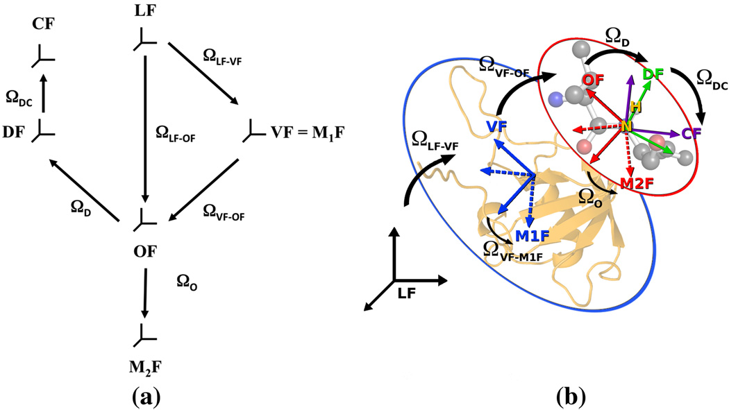
The various reference frames that define the SRLS model in this study are shown in Figure 2a. Their association with the appropriate features of the protein structure, with the N–H bond acting as probe, is illustrated in Figure 2b. The laboratory LF frame is space-fixed with its z-axis aligned along the external magnetic field. The global diffusion frame, M₁F, is fixed in the protein. The local director frame, VF, is fixed in the protein. The global diffusion is taken isotropic in this study; in this case M₁F and VF are the same. OF is the frame in which the local ordering tensor is diagonal, and M₂F is the frame in which the local diffusion tensor is diagonal. Both OF and M₂F are fixed in the probe.

Figure 2.

(a) Reference frames defining the SRLS model LF – laboratory frame; VF – local director frame, same as isotropic global diffusion frame, M₁F, fixed in the protein; OF – local ordering frame, fixed in the probe; M₂F – local diffusion frame, fixed in the probe DF – ¹⁵N-¹H dipolar magnetic frame, fixed in the probe; CF – ¹⁵N CSA frame, fixed in the probe. The Euler angles corresponding to the respective frame transformations are also depicted. The angles Ω_LF−VF, Ω_LF−OF and Ω_VF−OF are time-dependent. (b) Same reference frames as in part (a), associated with the appropriate features of the protein structure.

The magnetic ¹⁵N–¹H dipolar tensor frame, DF, and the magnetic ¹⁵N CSA tensor frame, CF, are fixed in the probe. The Euler angles for rotation from OF to DF are given by Ω_D, from OF to M₂F by Ω_O, and from DF to CF by Ω_DC. In this study Ω_D and Ω_Oare determined by data fitting; Ω_DC and the principal values of the magnetic tensors are assumed to be known and constant (Refs. ^44–46).

The time-dependent Euler angles, Ω_LF−OF(t), are modulated by the local and global motions. The time-dependent Euler angles Ω_LF−M1F(t), or in this case Ω_LF−VF(t), are modulated by the global tumbling. For describing the local motion we use a coupled representation; that is, we introduce the stochastic variable Ω_VF−OF(t) = Ω_LF−OF(t) − Ω_LF−VF(t) describing the relative orientation of the probe with respect to the protein.^{34,36,37,42,43} The two rotators are coupled by the potential U(Ω_VF−OF). The diffusion equation for the coupled system is given by:

$$\frac{\partial }{\partial t}P(\mathbf{X},t)=-\widehat{\mathrm{\Gamma }}P(\mathbf{X},t)$$ (1)

where X = Ω_VF−OF,Ω_LF−VF) is a set of coordinates completely describing the system and^{34,36,37,42,43}

$$\widehat{\mathrm{\Gamma }}={\mathbf{Ĵ}}^{\mathit{\text{tr}}}({\mathrm{\Omega }}_{\text{VF}-\text{OF}}){\mathbf{D}}_2{P}_{\text{eq}}(\mathbf{X})\mathbf{Ĵ}({\mathrm{\Omega }}_{\text{VF}-\text{OF}})P_{\text{eq}}^{-1}(\mathbf{X})+{[\mathbf{Ĵ}({\mathrm{\Omega }}_{\text{VF}-\text{OF}})-\mathbf{Ĵ}({\mathrm{\Omega }}_{\text{LF}-\text{VF}})]}^{\mathit{\text{tr}}}{\mathbf{D}}_1{P}_{\text{eq}}(\mathbf{X})[\mathbf{Ĵ}({\mathrm{\Omega }}_{\text{VF}-\text{OF}})-\mathbf{Ĵ}({\mathrm{\Omega }}_{\text{LF}-\text{VF}})]P_{\text{eq}}^{-1}(\mathbf{X})$$ (2)

with Ĵ(Ω_VF−OF) and Ĵ(Ω_LF−VF) representing the angular momentum operators for the probe and the protein, respectively.

The Boltzmann distribution is P_eq (X) = (1/8π²)exp[−U(Ω_VF−OF)/k_BT]/〈exp[−U(Ω_VF−OF)/k_BT]〉. The potential U(Ω_VF−OF) is in general expanded in the full basis set of the Wigner rotation matrix elements. When only the rank 2 terms are preserved, one has^34,36,37

$$u\left({\mathrm{\Omega }}_{\text{VF}-\text{OF}}\right)=U\left({\mathrm{\Omega }}_{\text{VF}-\text{OF}}\right)/k_{B}T=-c_0^2{D}_{0,0}^2\left({\mathrm{\Omega }}_{\text{VF}-\text{OF}}\right)-c_2^2\left[D_{0,-2}^2\right({\mathrm{\Omega }}_{\text{VF}-\text{OF}})+D_{0,2}^2({\mathrm{\Omega }}_{\text{VF}-\text{OF}}\left)\right].$$ (3)

The order parameters, $S_0^2=\langle D_{0,0}^2\left({\mathrm{\Omega }}_{\text{VF}-\text{OF}}\right)\rangle \text{ and }{S}_2^2=\langle D_{0,2}^2\left({\mathrm{\Omega }}_{\text{VF}-\text{OF}}\right)+D_{0,2}^2\left({\mathrm{\Omega }}_{\text{VF}-\text{OF}}\right)\rangle$, depend on the coefficients $c_0^2\text{ and }{c}_2^2$ in view of averaging 〈f〉 = ∫ dXP_eq (X) f (X), where the integral is extended to the whole volume of phase space.^36,37

Expansion terms corresponding to rank 4 Wigner matrix elements have been also included in our most recent computational scheme.^42,43 They allow a more detailed modeling, in particular diffusion within two wells with less frequent jumps between them.^32,52 More general multi-potential-well models may be included by adding appropriate terms in the expansion of U(Ω_VF−OF). However, in this study we employ the simplest potential given in eq 3.

An NMR experimental observable is expressed as a two-time autocorrelation function of rank 2 Wigner matrix elements in the time-dependent Euler angles that describe the orientation Ω_µ of the µ-th magnetic tensor (µ might represent a dipolar, chemical shift anisotropy, or quadrupolar tensor) with respect to the laboratory frame, which in turn can be obtained from Ω_LF−OF(t) and Ω_LF−VF(t)

$$C_{\mathrm{\mu }}(t)=\langle D_{0,0}^{2*}({\mathrm{\Omega }}_{\mathrm{\mu }}(t))D_{0,0}^2({\mathrm{\Omega }}_{\mathrm{\mu }}(0))\rangle =\langle D_{0,0}^2\left({\mathrm{\Omega }}_{\mathrm{\mu }}\right)\left|e^{-\widehat{\mathrm{\Gamma }}t}\right|D_{0,0}^2\left({\mathrm{\Omega }}_{\mathrm{\mu }}\right)P_{\mathit{\text{eq}}}\rangle .$$ (4)

In this study only dipolar ¹⁵N-¹H and ¹⁵N CSA interactions are considered. Eq 4 can be evaluated numerically by adopting the Smoluchowski form of the time evolution operator Γ̂ given by eq 2.

Following a standard approach^36,37,42,43 we span Γ̂ over a complete set of basis functions, Consequently eq 4 is transformed into a multi-exponential decay C_µ(t) = ∑_ic_µ,i exp (−t/τ_µ,i). The correlation time, τ_µ,i, denotes the inverse of a given eigenvalue of Γ̂. The corresponding weighting factor, c_µ,i, is obtained from the eigenvector corresponding to τ_µ,i. A more detailed description of the SRLS model and the solution of eq 2 can be found elsewhere.^33,42,43

The Fourier Transform of the time correlation function of eq 4 is the spectral density $J_{\mathrm{\mu }}(\mathrm{\omega })={\displaystyle {\sum }_{\mathrm{i}}\frac{c_{\mathrm{\mu },\mathrm{i}}{\mathrm{\tau }}_{\mathrm{\mu },\mathrm{i}}}{1+{\mathrm{\omega }}^2{\mathrm{\tau }}_{\mathrm{\mu },\mathrm{i}}^2}}$. The expressions for ¹⁵N T₁, T₂ and ¹⁵N–{¹H} NOE are obtained as a function of the ¹⁵N–¹H dipolar and ¹⁵N CSA auto-correlated spectral densities, according to standard expressions of the Redfield theory.^10,53,54

The SRLS program has been integrated⁴⁹ with a hydrodynamics-based approach for calculating D₁, within a C++ parallelized and object-oriented code, which show an increase in efficiency of approximately one order of magnitude relative to the fitting scheme developed in Ref. 36.

We call this software package C⁺⁺OPPS (COupled Protein Probe Smoluchowski).^42,43 C⁺⁺OPPS is distributed under the GNU Public License (GPL) v2.0. The software is available at the website http://www.chimica/unipd.it/licc/software.html.

The following comment is in order. The SRLS approach is an extension of the established approaches for the treatment of restricted motions in liquids,^11,12 which are themselves extensions of the classical approach set forth in early work.¹⁰ The established approaches to which we refer treat a rigid spin-bearing molecule reorienting in the presence of a potential of mean torque (POMT) exerted by a locally anisotropic (liquid-crystalline (LC)) medium. SRLS treats rigid spin-bearing probes reorienting in the presence of a POMT of similar form exerted by the immediate protein surroundings at the site of the motion of the probe. For a frozen protein SRLS reproduces the main features of the established approaches.³⁷ When the protein is allowed to reorient, a two-body coupled-rotator scenario emerges; the motion of the protein is also included in the formalism, and the POMT represents the coupling potential. The simple MF limit of SRLS, the general SRLS theory, and the LC approaches are summarized in Ref. 37, where also analogies and differences are outlined.

2.2. The global diffusion tensor

A hydrodynamics-based mesoscopic method is used, which avoids in part the atomistic description of the diffusing molecule and describes the solvent as a continuum.⁴⁹ This method is in principle applicable to molecules that are large enough with respect to the solvent molecules so that specific solute-solvent interactions become unimportant. This is usually assumed for proteins, even if specific interactions are not always negligible. An example is the so called dielectric friction correction to the friction tensor.^55,56 However, it has been shown by various authors that a relative simple hydrodynamics approach can give very good agreement with the dissipative properties of proteins when an appropriate choice is made for a single free parameter, related to the solvent exposed surface.^49,57–59

The hydrodynamics-based model implemented in C⁺⁺OPPS describes the molecular structure as an ensemble of spheres, each representing a non-hydrogen atom.⁴⁹ The friction tensor, ξ, of the system of unconstrained spheres (unbounded atoms) is defined as follows. Based on the Stokes-Einstein relation, the diagonal elements of ξ are given as ξ_ii = CπηR_i, where C is 4 for stick and 6 for slip boundary conditions, η is the solvent viscosity and R_i is the effective radius of the i-th sphere. The out-of-diagonal elements of ξ, which describe the hydrodynamic interactions among spheres, are calculated using the standard Rotne-Prager model.⁶⁰ The translational force (f) and the translational velocity (v) of the unconstrained spheres are related as f = −ξv By analogy, the dissipative force (F) acting on the molecule, and its generalized velocity (V), are related as F = − ΞV, where Ξ is the friction tensor of the molecule. Using standard classical mechanics it is straightforward to generate a geometric matrix, B, such that v = BV.^49,57 Using the fact that F = B^trf, the relation between the constrained (molecule-related) and unconstrained friction tensors is given by Ξ = B^trξB. The diffusion tensor, D = k_BTΞ⁻¹, comprising both translational and rotational contributions, is calculated using the Einstein relation. Only the rotational part is required by the SRLS model. A code that implements this theory as a standalone tool has been made available under the name DITE (DIffusion TEnsor).⁴⁹

2.3. The potential of mean force

A number of methods for determining POMT acting on a number of coordinates which are slow relative to the remaining degrees of freedom of the system have been developed. The simplest approaches use unbiased trajectories; the Boltzmann probability distribution is determined using nonparametric methods, e.g., histograms or kernel density estimators.^61,62 They require a highly efficient sampling of the phase space because the convergence of these estimators is slow for a set of correlated points, such as encountered in Markov processes.⁶³ More advanced methodologies apply a biasing potential or force to the coordinates of interest to better sample the phase space. Examples include umbrella sampling,^17,18 metadynamics^19,20 and adaptive biasing force dynamics.^21,22 Under certain conditions the bias can be related to the Helmholtz free energy (hence, the POMT) along the chosen coordinates. Applying these methodologies to the evaluation of the relevant SRLS-related parameters can be cumbersome because the reaction coordinates are not easily defined by the Euler angles that describe the relative orientation of the two bodies, Ω_VF−OF(t), using standard MD software packages.

We select a third simple route. It is postulated that the phenomenological SRLS potential of eq 3 is a reasonable approximation to the POMT.³⁶ In this case it is not necessary to determine the Boltzmann probability distribution from the MD trajectory; only two potential coefficients, $c_0^2\text{ and }{c}_2^2$, which define u(Ω_VF−OF), are required. The following procedure is used, based on the direct calculation of order parameters from the MD trajectory. In the first step, for each snapshot a protein-fixed frame, PF, is defined as the frame that diagonalizes the inertia tensor and has its origin on the center of mass of the protein. The trajectory is then related to this frame by application of the appropriate roto-translation to the original Cartesian coordinates in the laboratory frame (LF).

In the second step we select a reference structure from the trajectory. This is the equilibrium structure representative of the geometry of the molecule in solution. To select this structure we perform a k-clustering of the snapshots based on the backbone torsional angles. The snapshot closer to the centre of the most populated (statistically more representative) cluster is chosen.

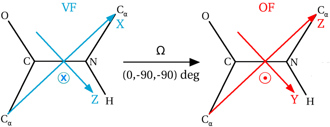
In the third step, the protein-fixed local director, VF, is defined on the reference structure for each N–H site. As found in previous work, where $c_0^2\text{ and }{c}_2^2$ were allowed to vary in the fitting process, N–H bonds that reside in internally mobile protein, domains^36,37,42,43 have β_D nearly −101.3°. The latter is the canonical angle between N–H and C^α–C^α (ref ⁶⁴). This is consistent with MD studies^65–67 and the 3D Gaussian Axial Fluctuations (GAF) model.⁶⁸ Within the scope of the frames of Figures 2 and 3, and the potential given in eq 3, X_VF is parallel to C^α–C^α, and Z_VF lies in the peptide-bond plane perpendicular to C^α–C^α. This geometric scenario, called “x-ordering”,⁶⁹ is used in the present study. The rotation matrix R_PF−VF is obtained from the atomic coordinates.

Figure 3.

Most probable orientation of the local ordering frame, OF, relative to the local director frame, VF, for the scenario in which the z-axis of the local ordering tensor, S, is parallel to C^α–C^α, and the potential is given by eq 3.

It is now straightforward to specify the equilibrium orientation of OF. In the reference structure the minimum energy configuration for OF is obtained by applying the rotation (0°, −90°, −90°) to VF (cf. Figure 3). Z_OF is parallel to C^α–C^α, and Y_OF lies in the peptide-bond plane perpendicular to C^α–C^α. This convention is used to orient OF on each N–H site in the snapshots.

In the final step, the time dependent rotation matrix R_PF−OF(t) is extracted directly from the trajectory. The required time dependent rotation matrix R_VF−OF(t) is finally obtained as:

$${\mathbf{R}}_{\text{VF}-\text{OF}}(t)={\mathbf{R}}_{\text{PF}-\text{OF}}(t){\mathbf{R}}_{\text{PF}-\text{VF}}^{\text{tr}}={\mathbf{E}}^{\mathit{\text{tr}}}({\mathrm{\Omega }}_{\text{VF}-\text{OF}}(t)),$$ (5)

where E^tr(Ω_VF−OF(t)) is the matrix from which the time series of the Euler angles Ω_VF−OF(t) are obtained. The following autocorrelation functions are then calculated

$$C_0^2(t)=\langle D_{0,0}^{2*}({\mathrm{\Omega }}_{\text{VF}-\text{OF}}(t))D_{0,0}^2({\mathrm{\Omega }}_{\text{VF}-\text{OF}}(0))\rangle$$ (6)

and

$$C_2^2(t)=\langle {\left[D_{0,-2}^2\right({\mathrm{\Omega }}_{\text{VF}-\text{OF}}(t))+D_{0,2}^2({\mathrm{\Omega }}_{\text{VF}-\text{OF}}(t)\left)\right]}^{*}\left[D_{0,-2}^2\right({\mathrm{\Omega }}_{\text{VF}-\text{OF}}(0))+D_{0,2}^2({\mathrm{\Omega }}_{\text{VF}-\text{OF}}(0)\left)\right]\rangle .$$ (7)

Since for a generic autocorrelation function G(t) = 〈f(t)f(0)〉 one has that lim_t→∞ G(t) = (〈f〉)² where 〈f〉 is the equilibrium average of observable f(t), the following expressions are valid:

$$S_0^2(c_0^2,c_2^2)={\displaystyle \int d{\mathrm{\Omega }}_{\text{VF}-\text{OF}}{D}_{0,0}^2\left({\mathrm{\Omega }}_{\text{VF}-\text{OF}}\right)P_{\text{eq}}({\mathrm{\Omega }}_{\text{VF}-\text{OF}},}{c}_0^2,c_2^2)\cong -\sqrt{{\text{lim}}_{t\to \infty }{C}_0^2(t)}={\left(S_0^2\right)}_{\text{MD}}$$ (8)

and

$$S_2^2(c_0^2,c_2^2)={\displaystyle \int d{\mathrm{\Omega }}_{\text{VF}-\text{OF}}\left[D_{0,-2}^2\right({\mathrm{\Omega }}_{\text{VF}-\text{OF}})+}{D}_{0,2}^2\left({\mathrm{\Omega }}_{\text{VF}-\text{OF}}\right)\left]P_{\text{eq}}\right({\mathrm{\Omega }}_{\text{VF}-\text{OF}},c_0^2,c_2^2)\cong -\sqrt{{\text{lim}}_{t\to \infty }{C}_2^2(t)}={\left(S_2^2\right)}_{\text{MD}}.$$ (9)

The first equality in eq 8 (eq 9) represents the definition of $S_0^2(S_2^2)$ (cf. eqs 3 and 4). The approximate equalities in eqs 8 and 9 indicate that within a good approximation the time correlation functions $C_0^2(t)\text{ and }{C}_2^2(t)$ decay to plateau values. Given the ambiguity associated with the square root, we selected the negative sign based on previous work.^36,37 Equations 8 and 9 represent a non linear system of two equations in two variables. The solution can be found numerically, e.g. using Powell's method, by searching for $\left[c_0^2,c_2^2\right]$ such that:

$$\{\begin{array}{c}{S}_0^2(c_0^2,c_2^2)-{\left(S_0^2\right)}_{\text{MD}}=0\hfill \\ S_2^2(c_0^2,c_2^2)-{\left(S_2^2\right)}_{\text{MD}}=0\hfill \end{array}$$ (10)

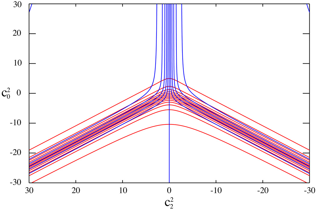
It is important to ascertain that the solution is unique. We show in Figure 4 contour plots of the two functions $S_0^2\left(c_0^2,c_2^2\right)\text{ and }{S}_2^2\left(c_0^2,c_2^2\right)$. A single order parameter can obviously not provide both $c_0^2\text{ and }{c}_2^2$. On the other hand, isolines of $S_0^2\text{ and }{S}_2^2$ intersect in one point only; this means that if a solution exists for eq 10, it will be unique.

Figure 4.

Isolines of the surfaces of $S_0^2$ (red) and $S_2^2$ (blue) as a function of the potential coefficients $c_0^2\text{ and }{c}_2^2$. Each couple of isolines intersects in one point only, illustrating the uniqueness of the solution of the non-linear system of equations in eq 10, provided a solution exists.

Two matters require additional comments. The first matter is related to the “real” orientation of VF (or OF). Because we postulate a functional shape for the potential, we know (and impose) a priori the relative orientation of VF and OF that corresponds to the minimum potential energy. For this reason, the order parameters are independent of the choice of the orientation of VF on the protein. In other words, if we apply the same rotation to VF and OF, the potential will not change, being defined with respect to the relative orientation between the two frames. Thus, the current approach does not permit extracting the orientation of either frame.

The second matter pertains to the effective potential of mean force. In principle, if the Boltzmann probability distribution is determined from the MD trajectory, given arbitrary orientations of the two frames VF and OF, the potential of mean force could be obtained, e.g. by fitting the general expansion $u\left({\mathrm{\Omega }}_{\text{VF}-\text{OF}}\right)={\displaystyle {\sum }_{\mathrm{j},\mathrm{m},\mathrm{k}}{\mathrm{u}}_{\mathrm{m},\mathrm{k}}^{\mathrm{j}}{D}_{\mathrm{m},\mathrm{k}}^{\mathrm{j}}}\left({\mathrm{\Omega }}_{\text{VF}-\text{OF}}\right)$, with appropriate truncation based on convergence to an analytical expression of the numerical potential. However, in order to be consistent with previous work, we decided to use the simple shape given in eq 3.

To summarize, the time series of the three Euler angles giving the relative orientation between the two bodies are extracted from the MD trajectory. From these time series the time correlation functions given by eqs 6 and 7 are evaluated and from their plateau values the order parameters are obtained. Finally, the system of non-linear equations in eq 10 is solved numerically to obtain the potential coefficients.

3. Results and discussion: plexin–B1

The approach described above has been applied to the RhoGTPase binding domain of the plexin–B1 protein. A previous MF study of ¹⁵N relaxation data acquired at 14.1 and 18.8 T, and 298 K, singled out the loops L1 and L4, and the terminal chain segments, as highly flexible.⁵⁰ Using the ¹⁵N T₁/T₂-based method and the lowest energy structure from the NMR derived ensemble, 2JPH, a global diffusion tensor with trace tr{D₁}/3 = 1.93×10⁷ s⁻¹ (correlation time 8.6 ns), and anisotropy D_{1, ‖}/D_1,⊥ = 1.26, was determined.⁵⁰ The MF squared order parameters, S², emerged as quite unusual. Helix α₁, part of helix α₂, and the tight turn between strand β₂ and helix α₁, have S² values close to 1. The loop L1 has S² values of approximately 0.3. The loop L4 has S² values ranging from 0.2 to 0.8. The loop L2 displays an alternating S² pattern with some maxima as high as 0.95 and some minima as low as 0.25. The terminal chain segments with very small S² values (~0 – 0.4) are unusually lengthy. Altogether, the flexible part of the backbone is comparable in size to the “rigid” part. In globular proteins, S² is usually on the order of 0.85 for secondary structure elements, and rarely below 0.6 for loops.⁴ Typically, the “rigid” part of the protein backbone exceeds in size the flexible part. Thus, the S² pattern of plexin–B1 reflects intricate and quite unusual internal mobility.

3.1. Rotational diffusion tensor

The rotational diffusion tensor of the protein, D₁, was calculated using the DITE program⁴⁹ incorporated in the C⁺⁺OPPS package. The NMR derived structure 2JPH was used. As input parameters we employed an effective sphere radius of R = 2.0 Å, stick boundary conditions, C = 6, and water viscosity at 298.15 K of η = 8.9×10⁻⁴ Pa s. We obtained D_1,XX = 1.60×10⁷ s⁻¹, D_1,YY = 1.71×10⁷ s⁻¹ and D_1,ZZ = 2.47×10⁷ s⁻¹ as principal values of D₁; they represent a nearly axial diffusion tensor with D_1,‖ / D_1,⊥ ~ 1.5. As pointed out above, 15N T₁/T₂ analysis yielded D_1,‖ / D_1,⊥ = 1.26. It was shown previously that proteins with substantial internal mobility in the form of moving domains^36–42 or large flexible loops⁷⁰ prevail in solution as ensembles of inter-converting structures which are best represented by an isotropic global diffusion tensor, D₁.^36–42,70 This line of reasoning applies to plexin–B1. It is supported by the relatively large difference between the D_1,‖ / D_1,⊥ values determined with the two methods mentioned above, which are expected to lead to similar results. We have shown that in the presence of substantial internal mobility the calculation of the tensor D₁ is very sensitive to the subset of 15N T₁/T₂ data used.^36,37,39 The latter should comprise a large number of "rigid" N–H bonds which are distributed evenly in space. Neither assumption is fulfilled by plexin–B1. We have also shown that the sensitivity of the SRLS analysis to D₁ axiality is significantly smaller that its sensitivity to the asymmetry of the local spatial restrictions (cf. Tables 10 and 11 of ref 36). Evidence that unaccounted for rhombicity of the local ordering tensor, S, can be absorbed by artificial axiality of the global diffusion tensor, D₁, appears in previous studies.^36,37,42

Based on the evidence and arguments presented above, we considered D₁ to be isotropic, with D₁ = 1.93×107 s⁻¹ taken from Ref. 50.

3.2. Potential coefficients

Four 110 ns long trajectories, starting with the same minimum energy structure of the NMR-restraint-derived ensemble,⁷¹ were generated with the software package NAMD,⁷² following previously established protocols.⁷³ The simulation parameters are given in Table 1. The analysis of the trajectories was carried out with various functionalities of the CHARMM software package.⁷⁴ The CHARMM27 all-atom potential function was used with the CMAP correction. For non-bonded interactions a cut-off of 12 Å was used. The standard Particle-Mesh Ewald method was used to calculate the long-range electrostatic interactions, and counter-ions were added to neutralize the system. The TIP3P model was used for the solvent water.

Table 1.

MD simulation parameters associated with the calculation of the four MD trajectories for plexin–B1. Additional details, and pertinent references, are given in the text.

Protein Data Bank file	2JPH (Ref. 71)
Protein charge	+2, neutralized by Cl− counterions
Number of water molecules	10418
Water molecule model	TIP3P
Cubic periodic box dimension	68.8701 Å
Ensemble	N (33171 atoms), p (1 atm), T (300 K)
Thermostat	Temperature coupling
Barostat	Nosé – Hoover Langevin piston (piston period 200 fs, piston decay 100 fs, piston temperature 300 K)
Non-bonded interactions cutoff	12 Å, smoothing switch at 10 Å
Pair list distance	13.5 Å
Electrostatics	PME
Time step of integration	2 fs
Coordinates and velocities saving frequency	2500 MD steps
Equilibration period	10 ns
Production period	100 ns

In each of the four calculated trajectories, the starting structure of plexin-B1 was immersed in a cubic box with a side length of 68.87 Å containing explicit water molecules. Periodic boundary conditions were applied. Subsequently the system was energy minimized, heated up and equilibrated. Different seeds were used for the initial velocity assignments. The time step employed was 2 fs and coordinates were saved for trajectory analysis very 5 ps. All of the bonds involving hydrogen atoms were kept rigid using the SHAKE algorithm. The Berendsen thermostat and the Langevin piston method were employed to run simulations at constant temperature (T = 300 K), and pressure (p = 1 atm). The simulations were run for 110 ns. The first 10 ns of the various trajectories were not used in the SRLS/MD analysis as this period was considered as an equilibration time, required for the stabilization of the RMSD that reflects on changes of the protein geometry with respect to the reference starting structure.

As mentioned in the previous section, a k-clustering strategy of the snapshots was used to select the reference structure and consequently to define the R_PF−VF rotation matrix for all the N–H sites. We used CHARMM to cluster the snapshots on the basis of backbone (φ, ψ) angles, with a maximum root mean square cutoff radius of 20°. We then selected the most highly populated, i.e., most probable (and presumably most representative) cluster. The structure closest to the cluster centre has been chosen to be the reference structure.

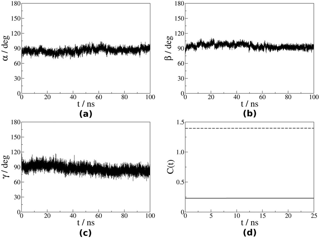
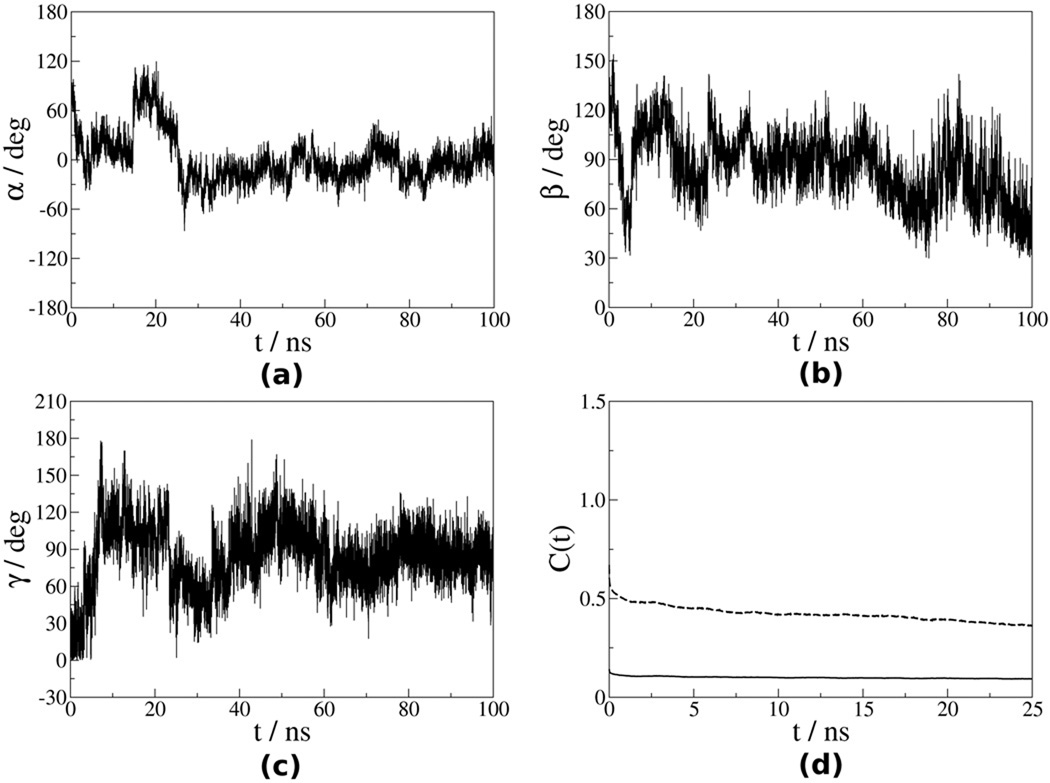
The time autocorrelation functions $C_0^2(t)\text{ and }{C}_2^2(t)$ (eqs 6 and 7) were calculated from the time series Ω_VF−OF (t) after discarding the first 10 ns of the trajectory. They decayed to plateau values within 25 ns, which represent one fourth of the trajectory length. The correlation functions have been averaged over the four trajectories and the emerging plateau values have been used to derive $S_0^2\text{ and }{S}_2^2$ (eqs 8 and 9). Figures 5 and 6 show the Euler angles α_VF−OF, β_VF−OF and γ_VF−OF for the N–H bonds of the residues Leu41 and Val86. The corresponding time correlation functions are also shown. For residue Leu41, which is located in the helix α₁ (Ref. ⁵⁰), the angles Ω_VF−OF exhibit limited fluctuations and the corresponding time correlation functions decay promptly to plateau values. For residue Val86, which belongs to a flexible loop, the angles Ω_VF−OF exhibit substantial fluctuations and the corresponding time correlation functions exhibit slower decays to plateau values.

Figure 5.

(a) – (c) Euler angles Ω_VF−OF (t) for the N–H bond of residue Leu41 extracted from the first (out of four) MD trajectory, as outlined in the text; (d) corresponding time correlation functions $C_0^2(t)$ (solid line) and $C_2^2(t)$ (dashed line).

Figure 6.

(a) – (c) Euler angles Ω_VF−OF (t) for the N–H bond of residue Val86 extracted from the first (out of four) MD trajectory, as outlined in the text; (d) corresponding time correlation functions $C_0^2(t)$ (solid line) and $C_2^2(t)$ (dashed line).

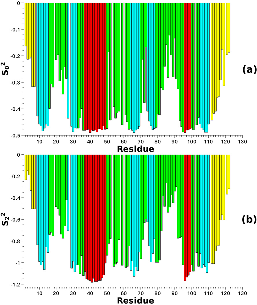
Figure 7 shows $S_0^2\text{ and }{S}_2^2$ as a function of residue number. Their ranges are $S_0^2\in (-0.5,1.0)\text{ and }{S}_2^2\in \left(-\sqrt{3/2},\sqrt{3/2}\right)$. The extreme values of these intervals represent the highest ordering and the highest tensor asymmetry, respectively. $S_0^2\text{ and }{S}_2^2$ determine the portion of the solid angle spanned by the N–H bond, i.e., the spatial confinement imposed on it by the immediate protein surroundings. The α-helices and β-sheets exhibit strong ordering and large tensor anisotropy. The loops L1 (Leu15–Gln25) and L4 (Leu77–Asn94), and the terminal chain segments, exhibit weaker ordering and reduced S tensor anisotropy. Based on the premise that high flexibility is required for binding, one may associate the loops L1 and L4 with this process. Indeed, the L4 region of plexin–B1 is adjacent to, or partially overlaps with the GTPase binding region in their complex.^50,75

Figure 7.

Order parameters $S_0^2$ (a) and $S_2^2$ (b) obtained from the molecular dynamics trajectory as a function of residue number. The colors distinguish among structural motifs: terminal chain segments (yellow), loops (green), β-sheets (cyan) and α-helices (red).

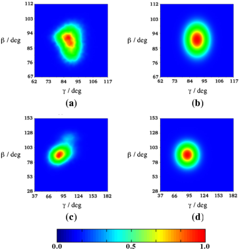
The equilibrium probability distribution function, $P_{\text{eq}}({\mathrm{\Omega }}_{\text{VF}-\text{OF}},c_0^2,c_2^2)$, used to calculate $S_0^2\text{ and }{S}_2^2$ is determined by the potential u(Ω_VF−OF) given by eq 3. This potential describes the energy landscape at the site of the motion of the N–H bond from a mean-field perspective. The potential energy function can be derived directly from the MD simulations and is related to the MD-calculated distribution as u(Ω_VF−OF) ≈ − ln [P_eq,MD (Ω_VF−OF)] + u₀, with u₀ a constant. Clearly, the potential in eq 3 is an approximation and to test its goodness we show in Figure 8 corresponding P_eq functions for residue Lys41, located in the α1 helix (Figures 8a,b), and residue Gln56, located in the L3 loop (Figures 8c,d). Figures 8a and 8c were obtained, as histograms, from the four trajectories. Figures 8b and 8d were generated using $c_0^2=-10.14\text{ and }{c}_2^2=-18.94$ as well as $c_0^2=-3.56\text{ and }{c}_2^2=-3.47$ for residues Lys41 and Gln56, respectively, obtained with eqs 6–10. Note that ${(S_0^2)}_{\text{MD}}({(S_2^2)}_{\text{MD}})$ in eqs 8–10 represents the square root of the plateau values of the time correlation function $C_0^2(t)(C_2^2(t))$.

Figure 8.

Equilibrium probability distribution functions P_eq,MD(Ω_VF−OF) calculated directly from the MD trajectories for residues Lys41 (a) and Gln56 (c). Distribution functions $P_{\text{eq}}({\mathrm{\Omega }}_{\text{VF}-\text{OF}},c_0^2,c_2^2)$ calculated with $c_0^2=-10.14\text{ and }{c}_2^2=-18.94$ for residue Lys41 (b), and $c_0^2=-3.56\text{ and }{c}_2^2=-3.47$ for residue Gln56 (d) (cf. eqs 6–10).

It can be seen that the P_eq functions shown in Figures 8a and 8b, or 8c and 8d, differ in that the SRLS functions are more regular. This approximation arises from the use of a relatively simple form of the potential, u(Ω_VF−OF), given by eq 3. In principle, enhancing the form of u(Ω_VF−OF) to better reproduce the local MD potential is straightforward (see Section 2.3.). The practicality of doing this will be explored in future work. At this time is may be concluded – based on Figure 8 – that the shape of the potential of mean force given by eq 3, and the utilization of the plateau values of $C_0^2\text{ and }{C}_2^2$ to evaluate $S_0^2\text{ and }{S}_0^2$, hence $c_0^2\text{ and }{c}_2^2$, are reasonable approximations.

3.3. SRLS analysis

Similar to the parameters obtained from hydrodynamics modeling and molecular dynamics, we assume the magnetic tensors to be known; from the literature one has δ_CSA = −169 ppm,⁴⁴ r_NH = 1.015 Å⁴⁵ and the tilt between the two magnetic frame, Ω_DC = (0°, −17°, 0°).⁴⁶

The parameters that still need to be evaluated are the principal values of the local diffusion tensor, D₂, the relative orientation of OF (S tensor frame) and DF (dipolar tensor frame), and the relative orientation of OF and M₂F (D₂ tensor frame). We assume that D₂ is axially symmetric, i.e., D_2,XX = D_2,YY = D_{2, ⊥}, D_2,ZZ = D_{2, ‖}; consequently we can set γ_O = 0°. Based on previous work,^36,37 we set γ_D = 0°. Six parameters are left: D_{2, ‖}, D_2,⊥, α_O, β_O, α_D and β_D. The following strategy is used in the data-fitting process: (1) D_{2, ⊥} and D_2,‖ are always allowed to vary; (2) we assume that within a given structural motif the four angles θ = (α_O, β_O, α_D, β_D) are on average the same. Four motifs are distinguished: α-helices, β-sheets, loops and terminal chain segments. Representative N–H bonds located within these motifs were analyzed to yield the results shown in Table 2. For α-helices and β-sheets we found that the sets θ_helix = (−62°, −90°, −90°, −101.3°) and θ_sheet = (0°, 0°, 0°, 0°) are appropriate. The loops and the terminal chain segments feature more complex local geometry. In most cases M₂F is collinear with one of the principal axes of OF; the angle β_D was found to vary.

Table 2.

Average Euler angles, Ω_o = (α_o,β_o,0) (OF → M₂F transformation), and Ω_D = (α_D,β_D,0) (OF → DF transformation) obtained by analyzing with the integrated approach developed herein several representative N–H bonds located in α-helices, β-sheets, loops and terminal chain segments. These data represent part of the input to scheme 1, where only D_2,⊥and D_2,‖ are allowed to vary (cf. Figure 1).

structural motifs	(αo,βo)/deg	(αD,βD)/deg
α-helix	(−62.0, −90.0)	(−90.0, −101.3)
β-sheet	(0.0, 0.0)	(0.0, 0.0)
loops and terminal chain segments	(0.0, 0.0) (0.0, −90.0) (−90.0, −90.0)	(−90.0, −71.3) (−90.0, −101.3)

Using the θ values shown in Table 2, the entire protein was fit with only D_{2, ⊥} and D_2,‖ allowed to vary. We call this 2-parameter fitting scenario scheme 1. As pointed out on many occasions (e.g., Refs. ³⁶ and ³⁷) two criteria, which must be fulfilled simultaneously, are used for the acceptance of results: physical viability and good statistics. Results that do not yield a physically sound and internally consistent picture of protein dynamics are not accepted. The statistical measure used has been χ²/df (with df the number of degrees of freedom); for the 2-parameter fitting scenario df = 4. Usually a critical value of 5% is used. Here we have used a critical value of 1%. The threshold has been decreased to account for the intricacy of the internal mobility of plexin–B1.⁵⁰ It corresponds to a relative error of 10% between theoretical and experimental relaxation parameters, which we consider to be realistic.

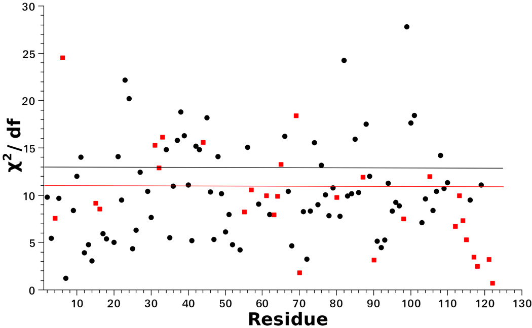
For residues with χ²/df exceeding the critical value of 1% the data-fitting procedure was extended to a 3-parameter fitting scenario, which we call scheme 2. Here D_{2, ⊥}, D_{2, ‖} and one of the θ angles were allowed to vary. In most of the cases good fits were obtained with the best-fit values of β_D, while in some cases α_O digressed somewhat from its value given in Table 2. Figure 9 shows χ²/df as function of residue number. For several N–H bonds χ²/df still exceeds the critical value of 1%. Allowing for yet another angle to vary did not improve the results. These are symptoms of over-fitting; better stochastic models, additional experimental data, and/or the determination of additional parameters with MD, are required.

Figure 9.

χ²/df (with df the number of degrees of freedom) for the fitting with scheme 1 (black circles) and scheme 2 (red squares). The horizontal lines represent the corresponding 1% critical χ²/df values used as statistical acceptance criteria for the results. For scheme 1, with df = 4, this value is ${\mathrm{\chi }}_{1\%}^2=13.28$ for scheme 2, with df = 3, this value is ${\mathrm{\chi }}_{1\%}^2=11.35$.

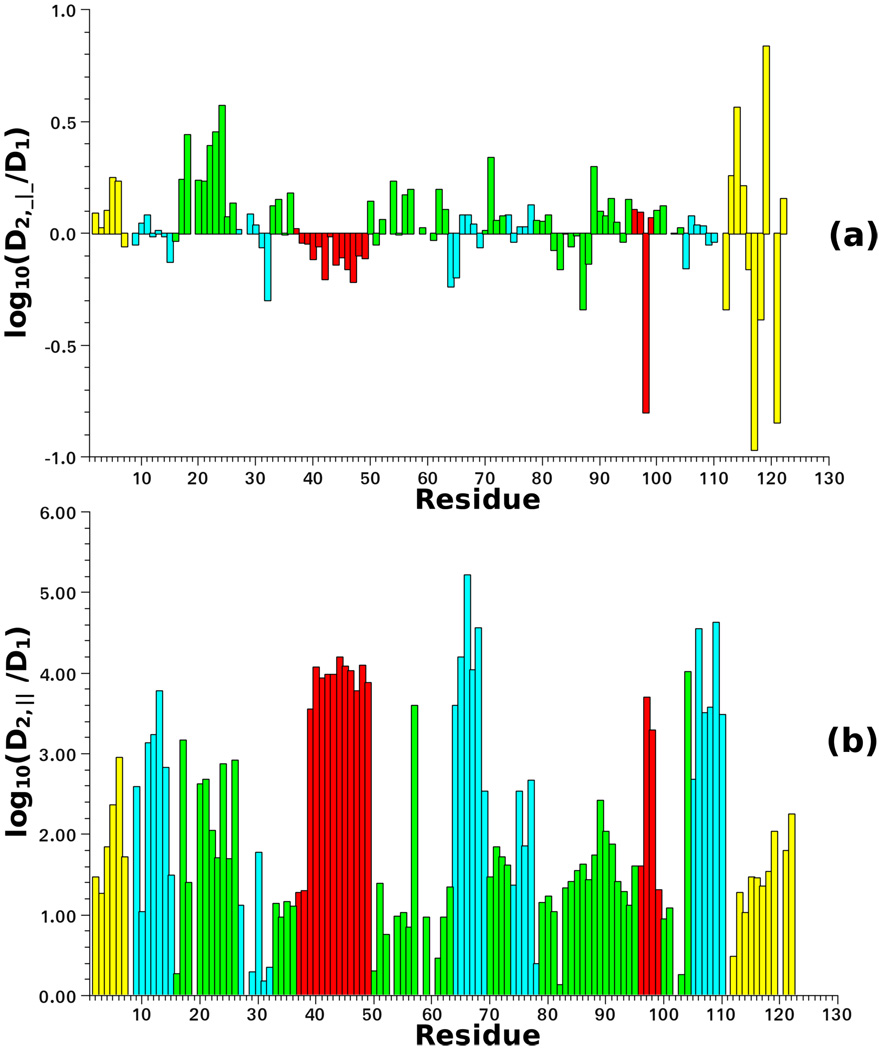
Figure 10 shows the best-fit values of log(D_{2, ⊥} / D₁) and log(D_2,‖ / D₁). It can be seen that D_{2, ⊥} is close in magnitude to D₁ (Figure 10a); in some cases, in particular for the helical regions and the C-terminal chain segment, D_{2, ⊥} is smaller than D₁. This might appear unphysical if one considers both the protein and the probe as “hydrodynamic” bodies rotating in the same medium, i.e., experiencing the same viscosity. In this case, the larger body (the protein) should feature higher friction. However, a purely hydrodynamic interpretation of the local diffusion is not altogether realistic. The local friction (diffusion) arises from “collisions” of the set of relevant coordinates with the remaining (protein + solvent) degrees of freedom, i.e., the thermal bath. Within this approach the complex local dynamics is translated to a local viscosity different from that of the solvent.⁷⁶

Figure 10.

log(D_{2, ⊥}/D₁) (a) and log(D_2,‖/D₁) (b) as a function of residue number. D₁ = 1.93×10⁷ s⁻¹ is the global diffusion rate. D_{2, ⊥} and D_2,‖ are the perpendicular and parallel components of the local diffusion tensor obtained by fitting with SRLS the ¹⁵N relaxation data of plexin–B1 acquired at 14.1 and 18,8 T, and 298 K,⁵⁰ as described in the text. The program C⁺⁺OPPS was used.⁴²,⁴³ The four colors distinguish among structural motifs: terminal chain segments (yellow), loops (green), β-sheets (cyan) and α-helices (red).

We recall that the correlation time for internal motion is given by τ₂ = 1/(6D₂), with D₂ = tr {D₂}/3 only in the absence of an external potential. For the simple case of a prolate top reorienting in the presence of a strong axial potential it was shown in early work^77,78 that the actual (“renormalized” by the strong potential) correlation time is given by ${\mathrm{\tau }}_{\text{ren}}~2{\mathrm{\tau }}_2/c_0^2$. Thus, τ_ren depends on both the friction (via D₂) and on the potential ($(\mathit{\text{via}}{c}_0^2)$). Although analytical relations do not exist outside of this simple limit, the actual correlation time depends on both the friction tensor and the coupling/restricting potential. Thus, one should not necessarily expect that D₂ be smaller than D₁. The physical constraint is that local motional correlation times be faster than the correlation time for global tumbling, in those cases when they are not (or poorly) coupled.

The parallel component of the local diffusion tensor, D_2,‖, is at least one order of magnitude larger than the global diffusion, D₁ (Figure 10b). There is clear distinction between α-helices and β-sheets on the one hand, and loops and terminal chain segments, on the other hand. For α-helices and β-sheets D_2,‖ is much larger than D₁, in some cases by four orders of magnitude. This mode may be interpreted as N–H wobbling. For loops and terminal chain segments log(D_2,‖ / D₁) is within the range of 1–2. A previous SRLS/ESR study of nitroxide-labeled T4 lysozyme found that D_{2, ⊥} > D_2,‖;⁷⁹ this has been interpreted as combined motion of the nitroxide and of the helix to which the label is attached. Such options should also be explored with SRLS/NMR.

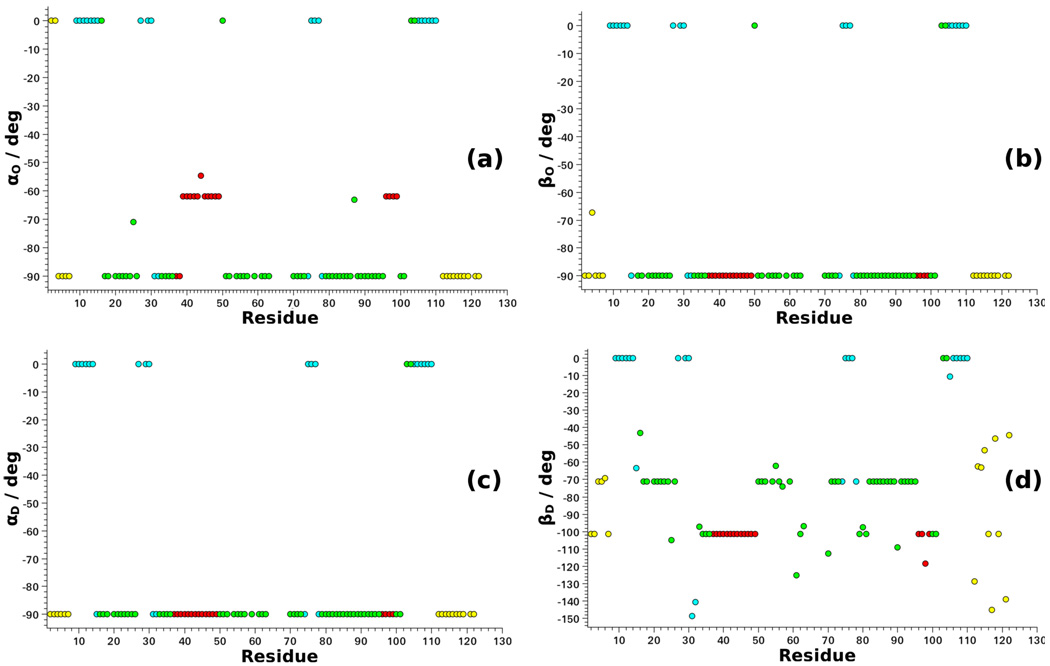
Figure 11 shows the values of the four angles, θ, as function of residue number. The polar (azimuthal) angle β_O (α_D) for the OF versus M₂F (OF versus DF) tilt differs for β-sheets, on the one hand, and all of the other structural motifs, on the other hand (Figures 11b,c). The azimuthal angle α_O for the OF versus M₂F tilt distinguishes among α-helices, β-sheets and loops/terminal chain segments (Figure 11a). The polar angle β_D for the OF versus DF tilt distinguishes among α-helices, β-sheets and loops/terminal chain segments, and illustrates the substantial diversity displayed by the latter (Figure 11d).

Figure 11.

Best-fit values of the angles θ = (α_O, β_O, α_D, β_D) obtained with SRLS data fitting of the ¹⁵N relaxation data of plexin–B1 acquired at 14.1 and 18,8 T, and 298 K,⁵⁰ as described in the text. The program C⁺⁺OPPS was used.⁴²,⁴³ The four colors distinguish among structural motifs: terminal chain segments (yellow), loops (green), β-sheets (cyan) and α-helices (red).

The following picture emerges. For α-helices the OF frame is oriented with the z-axis along the C^α–C^α axis; the y-axis lies within the peptide plane, nearly parallel to the N–H bond (Figure 3). This may be associated with crankshaft motion,^65,67 or internal peptide group motion.^64,66,68 For β-sheets the z-axes of the OF and M₂F frames are both parallel to the N–H bond. This might reflect implicitly motion involving the β-sheet; further investigation is required.

The orientation of the D₂ tensor in loops and the terminal chain segments cannot be associated at this time with specific structural elements.

The N–H bonds located in the chain segment Glu80–Phe90, corresponding to the loop L4, are characterized, similar to the terminal residues, by both low ordering (Figure 7) and slow local diffusion (Figure 10). This implies exploration of a larger region of conformational space while fluctuating slowly. Both properties provide a great adaptability, both in terms of structure and dynamics, to conformational rearrangements that might be required for binding. Further investigation of the flexible regions of the plexin–B1 backbone using more elaborate stochastic models is undoubtedly warranted.

It is of interest to compare the description of plexin–B1 dynamics by our integrated approach with its description by MF, previously published by one of us.⁵⁰ The intricate internal dynamics of plexin–B1 is described in MF in terms of a squared generalized order parameter, S², and a local motional correlation time, τ_e. The latter is on the order of 1–3 ns whereas the global motion occurs with an experimentally determined correlation time of 1/(6 D₁) = 8.6 ns. Mode-coupling, whereby the locally reorienting N-H bond follows the slower motion of the protein through the time dependence of Ω_VF−OF, is important when the local motion (1–3 ns) occurs on the same time scale as the global motion (8.6 ns).^31,34 MF does not account for this phenomenon. A single squared generalized order parameter (S²) cannot describe both the extent and the asymmetry of the local ordering. Yet, the asymmetry of the spatial restrictions at the site of the motion of the N–H bond in proteins has been shown to be important.^{35–42,64–68} As found with MD studies,^64–68 and with SRLS analyses,^35–42 the N–H sites in proteins are characterized by general features of local geometry.

Our integrated approach provides pairs of axial $(S_0^2)$ and rhombic $(S_2^2)$ order parameters for every examined N–H site in the protein. The parameter $S_0^2$ evaluates the strength of the local ordering and the parameter $S_2^2$ evaluates its rhombicity.^11,12 The local spatial restrictions can also be described by the local potential, u(Ω_VF−OF), which in turn defines $S_0^2\text{ and }{S}_2^2$.^{32,33,35–39} The potential yields the equilibrium probability distribution function from which one can calculate conformational entropy and other thermodynamic properties without any further assumption (this will be pursued in future work). Note that MF can only consider axial local potentials for entropy calculation because only a single squared generalized order parameter, S², is determined. The SRLS/MD analysis provides insightful geometric information – see Euler angles depicted in Figure 11. In MF these angles are implicitly equal to zero. A complete axial local motional diffusion tensor, D₂, including principal values (D_2,‖ and D_{2, ⊥}) and orientation (α_O and β_O), is provided. This detailed picture of the local motion should be compared with its description to the mathematically defined effective local motional correlation time, τ_e in MF. Our study shows that the experimental ¹⁵N relaxation data of plexin–B1 are sensitive (among others) to the tensorial properties of the local motion. It has been shown that activation energies for local motion can be derived from the principal values of the tensor D₂.⁴¹ This important information cannot be derived from t_e in MF because this parameter is typically very inaccurate (e.g., cf. Refs. ³ and ⁴). Finally, our integrated approach allows for further enhancements. To correlate parameters determined with this approach with the 3D structure of the protein more elaborate stochastic models are required which treat the internal molecular degrees of freedom in greater (atomistic) detail (cf. Ref. 25).

Thus, it may be concluded that our integrated approach has provided new insights into the backbone dynamics of plexin–B1. Moreover, this is a powerful new approach for analyzing NMR spin relaxation in proteins in general.

It should be pointed out that generalized order parameters have been calculated with MD, and used in the context of MF analysis, in Ref. 8. Local potentials and geometric features have been calculated with MD and combined with a stochastic treatment of nitroxide dynamics in T4 lysozyme in Ref. 80. References 81–84 may be consulted for a comprehensive approach where SRLS and MD are combined to study spin relaxation in nitroxide-labeled T4 lysozyme. A detailed discussion and comparison, also with the approach presented here is outside the scope of this article.

4. Conclusions

An integrated computational approach comprising hydrodynamics-based modeling of dissipative properties, molecular-dynamics-derived local mean field potentials, and a two-body stochastic model for treating coupled local/global dynamics within the scope of general tensorial properties, has been developed. This approach has been applied to ¹⁵N spin relaxation from the protein plexin–B1, the dynamic complexity of which has been pointed out by a previous MF analysis. New physically sound structural (local potentials/local ordering tensors), dynamic (local motional rates) and geometric (relative tensor frame orientations) information has been obtained. Strong local ordering with large asymmetry has been detected for α-helices and β-sheets. Weaker local ordering with smaller asymmetry has been detected for loops and terminal chain segments. For α-helices the z-axis of the local ordering frame was found to be parallel to the C^α–C^α axis. For β-sheets the z-axes of both the local ordering and the local diffusion tensors were found to be parallel to the N–H bond. Details are given in terms of specific tensorial properties. These observations point out significant differences in local motion, structure and geometry. Further theoretical developments, aimed at gaining insights about these features at the atomic level, are clearly required. The present study suggests that in the foreseeable future integrated computational approaches to NMR spin relaxation in proteins are likely to play a significant role.

References

- 1.Palmer AG. Chem. Rev. 2004;104:3623–3640. doi: 10.1021/cr030413t. [DOI] [PubMed] [Google Scholar]
- 2.Mittermaier A, Kay LE. Science. 2006;312:224–227. doi: 10.1126/science.1124964. [DOI] [PubMed] [Google Scholar]
- 3.Igumenova TI, Frederick KK, Wand AJ. Chem. Rev. 2006;106:1672–1699. doi: 10.1021/cr040422h. [DOI] [PMC free article] [PubMed] [Google Scholar]
- 4.Jarymowycz VA, Stone MJ. Chem. Rev. 2006;106:1624–1671. doi: 10.1021/cr040421p. [DOI] [PubMed] [Google Scholar]
- 5.Hall JB, Fushman D. J. Am. Chem. Soc. 2006;128:7855–7870. doi: 10.1021/ja060406x. [DOI] [PMC free article] [PubMed] [Google Scholar]
- 6.Loth K, Pelupessy P, Bodenhausen G. J. Am. Chem. Soc. 2006;127:6062–6068. doi: 10.1021/ja042863o. [DOI] [PubMed] [Google Scholar]
- 7.Wang T, Weaver DS, Cai S, Zuiderweg ERP. J. Biomol. NMR. 2006;36:79–102. doi: 10.1007/s10858-006-9047-4. [DOI] [PubMed] [Google Scholar]
- 8.Sheppard D, Li D-W, Godoy-Ruiz R, Bruschweiler R, Tugarinov V. J. Am. Chem. Soc. 2010;132:7709–7719. doi: 10.1021/ja101691s. [DOI] [PubMed] [Google Scholar]
- 9.Sheppard D, Spranger R, Tugarinov V. Prog. NMR Spectrosc. 2010;56:1–45. doi: 10.1016/j.pnmrs.2009.07.004. [DOI] [PubMed] [Google Scholar]
- 10.Abragam A. Principles of Nuclear Magnetism. London: Oxford University Press (Clarendon); 1961. p. 305. [Google Scholar]
- 11.Emsley JW. NMR of Liquid Crystals. Dorbrecht: Riedel Publishers; 1983. [Google Scholar]
- 12.Luckhurst GR, Veracini CA. The Molecular Dynamics of Liquid Crystals. The Netherlands: Kluwer Academic Publishers; 1994. [Google Scholar]
- 13.Trbovic N, Kim B, Friesner RA, Palmer AG., III Proteins. 2008;71:684–694. doi: 10.1002/prot.21750. [DOI] [PMC free article] [PubMed] [Google Scholar]
- 14.Maragakis P, Lindorf-Larssen K, Eastwood MP, Dror RO, Klepeis JL, Arkin IT, Jensen MO, Xu H, Trbovic N, Friesner RA, Palmer AG, III, Shaw DE. J. Phys. Chem. B. 2008;112:6155–6158. doi: 10.1021/jp077018h. [DOI] [PMC free article] [PubMed] [Google Scholar]
- 15.Wong V, Case DA. J. Phys. Chem. B. 2008;112:6013–6024. doi: 10.1021/jp0761564. [DOI] [PubMed] [Google Scholar]
- 16.Voelz VA, Bowman GR, Beauchamp K, Pande VS. J. Am. Chem. Soc. 2010;132:1526–1528. doi: 10.1021/ja9090353. [DOI] [PMC free article] [PubMed] [Google Scholar]
- 17.Torrie GM, Valleau JP. Chem. Phys. Lett. 1974;28:578–581. [Google Scholar]
- 18.Torrie GM, Valleau JP. J. Comp. Phys. 1977;23:187–199. [Google Scholar]
- 19.Laio A, Parrinello M. Proc. Nat. Acad. Sci. 2002;20:12562–12566. doi: 10.1073/pnas.202427399. [DOI] [PMC free article] [PubMed] [Google Scholar]
- 20.Marini F, Camilloni C, Provasi D, Broglia RA, Tiana G. Gene. 2008;422:37–40. doi: 10.1016/j.gene.2008.06.003. [DOI] [PubMed] [Google Scholar]
- 21.Darve E, Rodríguez-Gómez D, Pohorille A. J. Chem. Phys. 2008;128:144120–144132. doi: 10.1063/1.2829861. [DOI] [PubMed] [Google Scholar]
- 22.Minoukadeh K, Chipot C, Leliévre T. J. Chem. Theory Comput. 2010;6:1008–1017. [Google Scholar]
- 23.Sugita Y, Okamoto Y. Chem. Phys. Lett. 1999;314:141–151. [Google Scholar]
- 24.Su L, Cukier RI. J. Phys. Chem. B. 2009;113:16197–16208. doi: 10.1021/jp903861a. [DOI] [PubMed] [Google Scholar]
- 25.Zerbetto M, Polimeno A, Kotsyubynskyy D, Ghalebani L, Kowalewski J, Meirovitch E, Olsson U, Widmalm G. J. Chem. Phys. 2009;131:234501–234510. doi: 10.1063/1.3268766. [DOI] [PubMed] [Google Scholar]
- 26.Buchete N-V, Hummer G. J. Phys. Chem. B. 2008;112:6057–6069. doi: 10.1021/jp0761665. [DOI] [PubMed] [Google Scholar]
- 27.Pietrucci F, Marinelli F, Carloni P, Laio A. J. Am. Chem. Soc. 2009;131:11811–11818. doi: 10.1021/ja903045y. [DOI] [PubMed] [Google Scholar]
- 28.Lipari G, Szabo A. J. Am. Chem. Soc. 1982;104:4546–4559. [Google Scholar]
- 29.Lipari G, Szabo A. J. Am. Chem. Soc. 1982;104:4559–4570. [Google Scholar]
- 30.Clore GM, Szabo A, Bax A, Kay LE, Driscoll PC, Gronenborn AM. J. Am. Chem. Soc. 1990;112:4989–4991. [Google Scholar]
- 31.Polimeno A, Freed JH. Adv. Chem. Phys. 1993;83:89–163. [Google Scholar]
- 32.Polimeno A, Freed JH. J. Phys. Chem. 1995;99:10995–11006. [Google Scholar]
- 33.Liang Z, Freed JH. J. Phys. Chem. B. 1999;103:6384–6396. [Google Scholar]
- 34.Tugarinov V, Liang Z, Shapiro YE, Freed JH, Meirovitch E. J. Am. Chem. Soc. 2001;123:3055–3063. doi: 10.1021/ja003803v. [DOI] [PubMed] [Google Scholar]
- 35.Meirovitch E, Shapiro YE, Liang Z, Freed JH. J. Phys. Chem. B. 2003;107:9898–9904. [Google Scholar]
- 36.Meirovitch E, Shapiro YE, Polimeno A, Freed JH. J. Phys. Chem. A. 2006;110:8366–8396. doi: 10.1021/jp056975t. [DOI] [PMC free article] [PubMed] [Google Scholar]
- 37.Meirovitch E, Shapiro YE, Polimeno A, Freed JH. Prog. Nucl. Magn. Res. Spectr. 2010;56:360–405. doi: 10.1016/j.pnmrs.2010.03.002. [DOI] [PMC free article] [PubMed] [Google Scholar]
- 38.Tugarinov V, Shapiro YE, Liang Z, Freed JH, Meirovitch E. J. Mol. Biol. 2002;315:155–170. doi: 10.1006/jmbi.2001.5231. [DOI] [PubMed] [Google Scholar]
- 39.Shapiro YE, Kahana E, Tugarinov V, Liang Z, Freed JH, Meirovitch E. Biochemistry. 2002;4:6271–6281. doi: 10.1021/bi012132q. [DOI] [PubMed] [Google Scholar]
- 40.Meirovitch E, Shapiro YE, Polimeno A, Freed JH. J. Phys. Chem. B. 2007;111:12865–12875. doi: 10.1021/jp072156s. [DOI] [PMC free article] [PubMed] [Google Scholar]
- 41.Shapiro YE, Kahana E, Meirovitch E. J. Phys. Chem. B. 2009;113:12050–12060. doi: 10.1021/jp901522c. [DOI] [PubMed] [Google Scholar]
- 42.Zerbetto M, Polimeno A, Meirovitch E. J. Phys. Chem. B. 2009;113:13613–13625. doi: 10.1021/jp9046819. [DOI] [PubMed] [Google Scholar]
- 43.Zerbetto M, Polimeno A, Meirovitch E. Int. J. Quantum Chem. 2010;110:387–405. [Google Scholar]
- 44.Damberg P, Jarvet J, Gräslund A. J. Am. Chem. Soc. 2005;127:1995–2005. doi: 10.1021/ja045956e. [DOI] [PubMed] [Google Scholar]
- 45.Yao L, Vögeli B, Ying J, Bax A. J. Am. Chem. Soc. 2008;130:16518–16520. doi: 10.1021/ja805654f. [DOI] [PMC free article] [PubMed] [Google Scholar]
- 46.Fushman D, Tjandra N, Cowburn D. J. Am. Chem. Soc. 1998;120:10947–10952. [Google Scholar]
- 47.Barone V, Polimeno A. Phys. Chem. Chem. Phys. 2006;8:4609–4629. doi: 10.1039/b607998a. [DOI] [PubMed] [Google Scholar]
- 48.Zerbetto M, Polimeno A, Barone V. Com. Phys. Com. 2009;180:2680–2697. [Google Scholar]
- 49.Barone V, Zerbetto M, Polimeno A. J. Comp. Chem. 2009;30:2–13. doi: 10.1002/jcc.21007. [DOI] [PubMed] [Google Scholar]
- 50.Bouguet-Bonnet S, Buck M. J. Mol. Biol. 2008;377:1474–1487. doi: 10.1016/j.jmb.2008.01.081. [DOI] [PMC free article] [PubMed] [Google Scholar]
- 51.Tong Y, Bagheri-Hamaneh PK, Penachioni M, Hota JY, Kim S, Alviani R, Shen L. J. Biol. Chem. 2009;284:35962–35972. doi: 10.1074/jbc.M109.056275. [DOI] [PMC free article] [PubMed] [Google Scholar]
- 52.Moro GJ, Polimeno A. J. Chem. Phys. 1997;107:7884–7893. [Google Scholar]
- 53.Peng JW, Wagner G. In: Methods in Enzymology. James TL, Oppenheimer NJ, editors. Vol. 239. New York: Academic Press; 1994. pp. 563–595. [Google Scholar]
- 54.Cavanagh J, Fairbrother WJ, Palmer AG, III, Skelton NJ, Rance M. Protein NMR Spectroscopy: Principles and Practice. New York: Academic Press; 2006. [Google Scholar]
- 55.Nee T-W, Zwanzig R. J. Chem. Phys. 1970;52:6353–6363. [Google Scholar]
- 56.Moro GJ, Nordio PL, Polimeno A. Mol. Phys. 1989;68:1131–1141. [Google Scholar]
- 57.Moro GJ. Chem. Phys. 1987;118:181–197. [Google Scholar]
- 58.de la Torre JG, Huertas ML, Carrasco B. Biophys. J. 2000;78:719–730. doi: 10.1016/S0006-3495(00)76630-6. [DOI] [PMC free article] [PubMed] [Google Scholar]
- 59.Ryabov YE, Geraghty C, Varshney A, Fushman D. J. Am. Chem. Soc. 2006;128:15432–15444. doi: 10.1021/ja062715t. [DOI] [PubMed] [Google Scholar]
- 60.Rotne J, Prager S. J. Chem. Phys. 1969;50:4831–4837. [Google Scholar]
- 61.Scott DW. Biometrika. 1979;66:605–610. [Google Scholar]
- 62.Izenman AJ. J. Am. Stat. Ass. 1991;86:205–224. [Google Scholar]
- 63.Hart JD. J. Am. Stat. Ass. 1984;79:110–117. [Google Scholar]
- 64.Lienin SF, Bremi T, Brutscher B, Brüschweiler R, Ernst RR. J. Am. Chem. Soc. 1998;120:9870–9879. [Google Scholar]
- 65.Fadel AR, Jin DQ, Montelione GT, Levy RM. J. Biomol. NMR. 1995;6:221–226. doi: 10.1007/BF00211787. [DOI] [PubMed] [Google Scholar]
- 66.Buck M, Karplus M. J. Am. Chem. Soc. 1999;121:9645–9658. [Google Scholar]
- 67.Clore GM, Schwieters CD. Biochemistry. 2004;43:10678–10691. doi: 10.1021/bi049357w. [DOI] [PubMed] [Google Scholar]
- 68.Bremi T, Brüschweiler R. J. Am. Chem. Soc. 1997;119:6672–6673. [Google Scholar]
- 69.Barnes JP, Freed JH. Biophys. J. 1998;75:2532–2546. doi: 10.1016/S0006-3495(98)77698-2. [DOI] [PMC free article] [PubMed] [Google Scholar]
- 70.Pang Y, Buck M, Zuiderweg ERP. Biochemistry. 2002;41:2655–2666. doi: 10.1021/bi011657f. [DOI] [PubMed] [Google Scholar]
- 71.Tong A, Hota PK, Bagheri-Hamaneh M, Buck M. Structure. 2008;16:246–258. doi: 10.1016/j.str.2007.12.012. [DOI] [PMC free article] [PubMed] [Google Scholar]
- 72.Phillips JC, Braun R, Wang W, Gumbart J, Tajkhorshid E, Villa E, Chipot C, Skeel RD, Kalé L, Schulten K. J. Comp. Chem. 2005;26:1781–1802. doi: 10.1002/jcc.20289. [DOI] [PMC free article] [PubMed] [Google Scholar]
- 73.Buck M, Bouguet-Bonnet S, Pastor RW, MacKerell AD. Biophys. J. 2006;90:L36–L39. doi: 10.1529/biophysj.105.078154. [DOI] [PMC free article] [PubMed] [Google Scholar]
- 74.Brooks BR, Bruccoleri RE, Olafson BD, States DJ, Swaminathan S, Karplus M. J. Comp. Chem. 1983;4:187–217. [Google Scholar]
- 75.Loh AP, Guo W, Nicholson LK, Oswald RE. Biochemistry. 1999;38:12547–12557. doi: 10.1021/bi9913707. [DOI] [PubMed] [Google Scholar]
- 76.Chakraborty S, Bandyopadhyay SJ. J. Phys Chem. B. 2007;111:7626–7630. doi: 10.1021/jp072350e. [DOI] [PubMed] [Google Scholar]
- 77.Polnaszek CF, Bruno GV, Freed JH. J. Chem. Phys. 1973;58:3185–3199. [Google Scholar]
- 78.Polnaszek CF, Freed JH. J. Phys. Chem. 1975;79:2283–2308. [Google Scholar]
- 79.Liang Z, Lou Y, Freed JH, Columbus L, Hubbell WL. J. Phys. Chem. B. 2004;108:17649–17659. [Google Scholar]
- 80.Budil DE, Sale KL, Khairy KA, Fajer PG. J. Phys. Chem. B. 2006;110:3703–3713. doi: 10.1021/jp054738k. [DOI] [PubMed] [Google Scholar]
- 81.Sezer D, Freed JH, Roux B. J. Am. Chem. Soc. 2009;131:2597–2605. doi: 10.1021/ja8073819. [DOI] [PMC free article] [PubMed] [Google Scholar]
- 82.Sezer D, Freed JH, Roux B. J. Chem. Phys. 2008;128:165106–165116. doi: 10.1063/1.2908075. [DOI] [PMC free article] [PubMed] [Google Scholar]
- 83.Sezer D, Freed JH, Roux B. J. Phys. Chem. B. 2008;112:11014–11027. doi: 10.1021/jp801608v. [DOI] [PMC free article] [PubMed] [Google Scholar]
- 84.Sezer D, Freed JH, Roux B. J. Phys. Chem. B. 2008;112:5755–5767. doi: 10.1021/jp711375x. [DOI] [PMC free article] [PubMed] [Google Scholar]