Bayesian models: the structure of the world, uncertainty, behavior, and the brain

Abstract

Experiments on humans and other animals have shown that uncertainty due to unreliable or incomplete information affects behavior. Recent studies have formalized uncertainty and asked which behaviors would minimize its effect. This formalization results in a wide range of Bayesian models that derive from assumptions about the world, and it often seems unclear how these models relate to one another. In this review, we use the concept of graphical models to analyze differences and commonalities across Bayesian approaches to the modeling of behavioral and neural data. We review behavioral and neural data associated with each type of Bayesian model and explain how these models can be related. We finish with an overview of different theories that propose possible ways in which the brain can represent uncertainty.

Introduction

What is the purpose of the nervous system or its parts? To successfully study a system, it is crucial to understand its purpose (see “computational level” in Ref. 1). This insight drives a line of research called normative models, which starts with an idea of what the objective of a given system could be and then derives what would be the optimal solution to arrive to that objective^a. The model predictions are then usually compared with the way the system actually behaves or is organized [2]. In this way, normative models can test hypotheses about the potential purpose of parts of the nervous system.

Uncertainty is relevant in most situations in which humans need to make decisions and will thus affect the problems to be solved by the brain. For example, we only have noisy senses, and any information that we sense must be ambiguous because we only observe incomplete portions of the world at any given time, or shadows of reality, as is beautifully illustrated by Plato’s allegory of the cave [3]. Therefore, it may be argued that a central purpose of the nervous system is to estimate the state of the world from noisy and incomplete data [4–5]. Bayesian statistics gives a systematic way of calculating optimal estimates based on noisy or uncertain data. Comparing such optimal behavior with actual behavior yields insights into the way the nervous system works.

Models in Bayesian statistics start with the idea that the nervous system needs to estimate variables in the world that are relevant (x) based on observed information (o), typically coming from our senses (e.g. audition, vision, olfaction). Bayes rule [6] then allows calculating how likely each potential estimate x is given the observed information o:

$$\text{p}(x\mid o)=\text{p}(o\mid x)\text{p}(x)/\text{p}(o)$$

For example, consider the case of estimating if our cat is hungry (x=“hungry”) given that it meowed (o=“meow”). If the cat usually meows if hungry (p(o|x)=90%), is hungry a quarter of the time (p(x)=25%), and does not meows frequently (p(o)=30%), then it is quite probably hungry when it meows (p(x|o)=90%×25%/30%=75%). If, on the other hand, the cat meows quite frequently (p(o)=70%), then the probability of being hungry if it meowed is much lower (p(x|o)=90%×25%/70%=32%). The formula above can also be seen as a way of updating the previous belief on the world, or prior (p(x)) by the current sensory evidence, or likelihood (p(o/x))^b.

Models using Bayes rule have been used to explain many results in perception, action, neural coding, and cognition. Bayesian models that have been used in these contexts have many different forms. The differences between these models derive from distinct assumptions about the variables in the world and the way they relate to one another. Each model is then the unique consequence of one set of assumptions about the world. However, all these Bayesian models share the same basic principle that different pieces of information can be combined in order to estimate the relevant variables.

Bayesian statisticians have developed a way of depicting how random variables relate to one another—by using graphical models [7–9]. We should mention here that several kinds of graphical models can be used [7–11]. Types of graphical models include Factor graphs, Markov Random Fields, ancestral graphs, and Bayesian network or directed acyclic graphs, which we discuss here. Bayesian networks/directed acyclic graphs are a type of graphical model that, besides indicating purely statistical relations, can be interpreted as a model of the causal structure in the world[9]. Therefore, we will use the Bayesian network class of graphical models to depict the different types of existing Bayesian models and structure this review.

In Bayesian networks, there are two kinds of random variables: those that are observed and those that are not observed. For example, we can hear our cat meow (observed variable) but we can never directly observe that it is hungry, only infer that from its behavior. Therefore, hunger is fundamentally an unobserved variable—unless some new neurophysiologic procedure is invented that measures Qualia. Unobserved variables are called latent or, as we will call it here, hidden. These hidden variables are typically estimated given the observed variables in Bayesian modeling.

There are many relevant reviews of and books about Bayesian methods. Some focus on cue combination [12–15], while others focus on general Bayesian estimation [8, 16–18], and yet others focus on the information integration for making choices [2, 19–20] or continuous control [21] and in possible representations of uncertainty [22]. These reviews provide excellent introductions into the mathematical treatment of estimation in various settings. Here, we want to instead focus on the structure each Bayesian model assumes about the world and give a taxonomy of these Bayesian models by focusing on the underlying graphical models.

Our review is structured as follows. In each section we will cover progressively more difficult problems to which Bayesian models are frequently applied. Each section starts with a simple example of the problem being dealt with and a graphical model that represents it, continues by making a short review of behavioral and modeling work related to that issue, and ends with available neural data that indicates where and how Bayesian computation can be occurring. We will end this review with an overview of proposals of how the brain may represent uncertainty.

Cue combination

Imagine that our cat ran away to avoid having a bath and is now hiding in the garden (Fig. 1A). It made the bushes move, providing a visual cue about its position, and meows, which provides an auditory cue. This is a typical example where one variable, the hidden location of the cat, is reflected in observed variables, in this case audition and vision, which are called cues.

Fig. 1.

Cue combination. A) Example of an indirect observation of a cat’s position. You can see the bush moving and hear a “meow” sound but you cannot directly observe the cat. Cartoon made by Hugo M. Martins. B) Graphical model of what is seen in A. The variable X (position of the cat) is unobserved, but it produces two observed variables: the moving bush, which provides a visual cue (O_v), and the “meow” sound, which provides an auditory cue (O_A).

In the graphical model associated with this example (Fig. 1B), the hidden variable (e.g. the cat’s position) that we want to estimate is assumed to independently cause the observed visual and auditory cues. The circle representing the cat’s position variable has no incoming arrows, indicating that there will be only a prior belief (p(position), see next section). The vision circle (O_v) has an incoming arrow from position, indicating that the probability of having a specific visual observation depends on the value of the position variable (p(vision | position)), i.e. the probability of seeing a specific bush moving depends on where the cat is hiding. Similarly, the audition circle (O_A) has an incoming arrow from position and we thus have p(audition|position). Jointly, these pieces of information define the joint probability distribution of the three random variables:

$$\text{P}(\text{position},\text{vision},\text{audition})=\text{p}(\text{position})\text{p}(\text{vision}\mid \text{position})\text{p}(\text{audition}\mid \text{position})$$

Importantly, the fact that there is no arrow directly connecting vision and audition indicates that, conditioned on the knowledge of position, vision and audition are independent. This can be seen as indicating that noise in vision is independent of noise in audition. This assumption about the way visual and auditory cues are generated may be true or not but it enables the construction of a simple normative model of behavior. The central assumptions about the world that give rise to each Bayesian model (in this case, the assumption of how cues are generated) can thus be effectively formalized in a graphical model.

In our example, we can say that the goal of our nervous system is to discover where the cat is, i.e. estimate the hidden variable, “position of the cat”. Assuming that this variable generated the observed visual and auditory cues, the nervous system has to invert this generative process and estimate the hidden variable position of the cat by combining the visual and auditory cues.

Bayesian statistics provides a way of calculating how to optimally combine the cues, i.e. a way of maximally reducing the final uncertainty about the cat’s position. The resulting estimate combines the cues, weighting them according to their reliability. If people combined cue information in a Bayesian way, the resulting estimate has less or equal uncertainty compared to the uncertainty associated with any of the cues.

This property of lower uncertainty in the final estimate is one of the crucial advantages of behavior that combines different pieces of knowledge in a way predicted by Bayesian models. Previously, it has been suggested that the Nervous System could use a winner-take-all approach, taking only into account the most reliable cue (in this case, generally vision) [23]. However, this would result in a final uncertainty generally higher than what would be obtained by employing Bayesian statistics^c. Furthermore, an approach in which only the most reliable cue is used cannot explain the cue interaction effects observed in daily life (for example, the McGurk effect- [24]).

Many experiments have probed how humans estimate hidden variables given more than one cue, and the results are in accordance to what would be predicted by Bayes theory [25–31]. The results of many of these studies have been framed in terms of Bayesian statistics, and these studies almost invariably assume the same graphical model (Fig. 1B). The typical experimental strategy is as follows. They first measure independently the uncertainties associated with each cue. Then, based on these estimates, they calculate what would be the weighting parameter (w) that would optimally combine both cues. They measure the way people actually combine cues when they have both cues available and compare the results with the model predictions^d. Importantly, the model predicts behavior in one condition (cue combination) based on the subject’s behavior in different situations (with only one cue).

Using an experimental setup like the one just described, Ernst and Banks have discovered that subjects use information from both vision and the sense of touch in order to estimate sizes, and they combine these cues in a way close to the statistical optimal [30]. Other studies also showed that the variability in the estimates obtained when subjects combined proprioceptive and visual information was smaller than the variability obtained when they could only use one of the senses, a phenomenon also predicted by Bayes theory [28]. Furthermore, they tended to rely more on the most accurate cue [27].

This close-to-optimal combination of different sensory cues has also been demonstrated in many other experiments and sensory modalities. For example, it has been found that subjects can combine optimally visual and auditory cues [32–33]. This combination is on the basis of the McGurk effect, in which when there is a discrepancy between what the lips of a person are saying and the actual sound, subjects hear a syllable that is a mix between the visual and the auditory syllable [24]. Cue combination has also been found within the visual system, with subjects combining cues of texture and motion [34], texture and binocular disparity [35–37], or even two texture properties [31] in order to estimate some position or slant. There is thus now ample evidence that in many if not most situations, cues are combined in a way close to the Bayesian optimal [31–37], which has been discussed in a good number of recent reviews [12–14, 38–41].

The cue combination studies we mentioned so far assume continuous cues and the estimation of continuous hidden variables, like the position of the hand or the distance of an object. However, there are also cases in which we want to estimate discrete variables—for example, how often someone has touched our hand or how often a light has flashed. In such cases, Bayesian models have also been shown to fit well human behavior [42–44]. The finding of near-optimal cue combination thus applies not only to continuous variables, but also to situations where discrete numbers are estimated

If people are Bayesian in their behavior, this means that the brain has to somehow represent and use uncertainty information for cue combination. How does the nervous system represent cues and their reliabilities to be able to combine them? We will discuss theoretical proposals of how the nervous system may represent uncertainty in the final section of this review, but focus now on available electrophysiological and imaging results specifically related to cue combination.

Many brain areas have been implied to participate in multisensory integration [for reviews, see Refs. 40, 45–46]. For example, in the Superior Colliculus (a brain area that receives visual, auditory and, somatosensory inputs), neuronal responses to a given sensory stimulus were influenced by the existence or nonexistence of other sensory cues [47]. Multisensory integration has also been analyzed in the superior temporal sulcus (STS), where it was found that, in a fraction of neurons responsive to the sight of an action, the sound of that action significantly modulated their visual response [48]. Neurons in the STS thus appear to form multisensory representations of observed actions. Further evidence of multisensory integration comes from imaging studies where activity in higher visual areas (hMT1/V5 and lateral occipital complex) of human subjects suggested combination of both binocular disparity and perspective visual cues, potentially in order to arrive at a unified 3D visual perception [49].

Bayesian models have inspired research on neurons in the dorsal part of the medial superior temporal area (MSTd) in the monkey. These neurons have been shown not only to integrate visual and vestibular sensory information, but also to do so in a way that closely resembles a Bayesian integrator, i.e. these neurons sum inputs linearly and subadditively (meaning that each cue weights one or less), and, moreover, the weights that they give to each cue change with the relative reliability of each cue [50–51].

Cue combination literature usually analyzes cases where the nervous system is likely to assume that there is a single hidden variable and multiple cues that are indicative about that variable. Both this variable and the observed variables may be continuous or discrete, bounded or unbounded (i.e. a distribution may be between 0 and 1 or −∞ and +∞), but the same graphical model describes all these models. While the models are different, the solution strategy is essentially the same—the probability distributions associated with each cue simply get multiplied together using Bayes rule. These models have been applied to many situations and describe the results of many experiments.

Combining a cue with prior knowledge

Even if only one cue is present, we can combine it with previous knowledge (prior) that we have about the hidden variable in order to better estimate it^e. In our example, if you can hear the cat but you cannot see it (Fig. 2A), you might still recall previous times in which the cat ran away to the garden: you have prior knowledge of probable positions of the cat, and can use it to estimate the cat’s position. Again, a hidden variable (position) causes the observed cue (the “meow” sound), a relation that can be formulated by a graphical model (Fig. 2B). In this case, estimates should depend on what we have learned in the past about the hidden variable (prior) and on our current observation (likelihood).

Fig. 2.

Combining a cue with prior knowledge. A) Example of an indirect observation of a cat’s position, but in which only a “meow” can be heard. B) Graphical model of what is seen in A. The variable X (position of the cat) is unobserved, but it produces the observed “meow” sound, which provides an auditory cue (O_A). C) Example of a visual illusion. Here people generally see one grove (left) and two bumps, but if the paper is rotated 180° then two groves and one bump are perceived. D) Checker-shadow illusion [54]. In this visual illusion, the rectangle A appears to be darker than B, while in reality they have the same color.

Indeed, standard Bayesian prior-likelihood experiments and cue combination experiments explained above are essentially based on the same graphical model and the mathematical treatment is analogous. The only difference is that in cue combination, there are at least two cues and priors are usually ignored and, in prior-likelihood experiments, the prior is incorporated but other potential cues are usually ignored. Priors can be considered a simple summary of the past information subjects have had in a particular task [52]. Moreover, they are independent of the current feedback, i.e. the prior is the information we get from all previous trials except the current one [53]. While it was generally ignored in previous models, including most of cue combination discussed above, prior knowledge clearly influences our decisions and even our perception of the world.

There are many examples of the effect of prior knowledge on perception. For example, in Figure 2C we can see one grove and two bumps, but if we rotate the paper by 180 degrees, their perceptual depth shifts (we see two groves and one bump instead). This occurs because people have the prior assumption that light should come from above. This is also beautifully illustrated in the Checker-shadow illusion, where the prior assumption of a light source that casts the observed shadow makes the rectangles A and B appear to have different brightness [54]. These sensory biases can then be explained with the incorporation of prior information on the final sensory perception.

Experimental studies have shown that priors can indeed be learned over time [52] and that they are independent of the current sensory feedback [53]. A diverse set of studies have also shown that people combine previously acquired knowledge (prior) with new sensory information (likelihood) in a way that is close to the optimum prescribed by Bayesian statistics. For example, when performing arm-reaching tasks [55–56], pointing tasks [57], or even timing tasks [58], people take into account both prior and likelihood information and, moreover, they do so in a way compatible with Bayesian statistics, given more weight to the more reliable “cue” or, in other words, they rely a lot on the prior when likelihood is relatively bad and vice versa [55–59].

As indicated by Bayes-like behavior when combining prior and likelihood, the brain needs to represent and use uncertainty of both previously acquired information and current sensory feedback in order to optimally combine these pieces of information. How does the nervous system represent prior and likelihood and their associated uncertainties? Currently, there is relatively little known about this (although some theories have been proposed; see the last section of this review). However, when it comes to movement, it has been found that the dorsal premotor cortex and the primary motor cortex encode multiple potential reaching directions, indicating a potential representation of priors [60–64]. However, we clearly do not understand yet how the nervous system integrates priors and likelihoods.

Combining information across time

In the previous sections, we discussed how information from multiple senses and from priors can be combined in order to arrive at better estimates about the world. However, many hidden variables in the world change over time—for example, the cat’s position is changing as the cat moves through the garden, and we obtain information about its whereabouts at different points in time (Fig. 3A). Such cases are captured by graphical models where the hidden variable exists with potentially different values as a function of time (Fig. 3B). The graphical model highlights the so-called Markov property: conditioned on the present state of the world, the past is independent from the future^f.

Fig. 3.

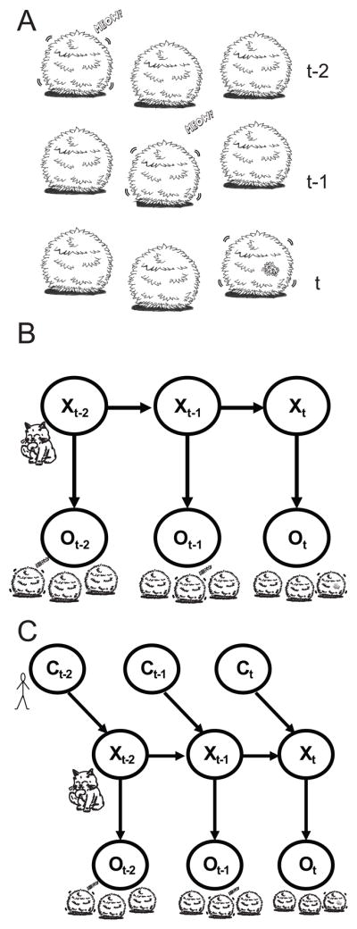
Combining information across time. A) Example of an indirect observation of a cat’s position, at different points of time (t-2, t-1 and t, being t the present time). B) Graphical model of what is seen in A. The hidden variable X (position of the cat) at each point of time produces a variable O that is observed. C) Graphical model similar to B, but in which the external effect of a Controller (in this case, a person) is incorporated in the model, which will affect X.

The situation and graphical model depicted in Figure 3 can be seen as an extension of the cue combination and prior likelihood models, but in which the hidden variable can change over time. Thus, at any point of time, the model is identical to the prior-likelihood integration model, and the joint estimate obtained at that point of time will then be the updated prior for the next point of time.

The graphical model in Fig. 3B underlies a range of related models. Models of this type that estimate discrete hidden variables are usually called Hidden Markov Models^g (HMM). When the variables are continuous and probability distributions are Gaussians, then the model is usually called a Kalman model [65]. When these models are used to make estimates about a given point of time, given only the past, they are generally called “filters;” when they make estimates given both past and future, they are called “smoothers.” Still, all these approaches share the same graphical model that specifies the Markov property and only differ in specific additional assumptions.

To make estimates, new sensory information obtained at each point of time needs to be combined with the current belief. A filter, e.g. the Kalman filter, can be seen as a system that alternates between two steps: (1) cues are combined with current beliefs using Bayes rule; and (2) the dynamics of the world (in our example, how fast the cat changes position) affect our estimates regarding the state of the world and thus our belief. Some of the dynamics are generally unpredictable making us less certain about the world (if the world is changing unpredictably we become uncertain about it), while the cues we receive generally make us more certain about the world. The interplay between unpredictable changes and observation defines uncertainty in such Bayesian models.

When we interact with the world, our movements also affect the dynamics of the world. This means that the state of the world at the next point in time depends on its previous state as well as our own state. For example, our own movements will affect the cat’s movements as well and therefore we should incorporate our own movements into the estimates. This situation is captured by the graphical model that underlies the Kalman controller (Fig. 3C). As the model retains the Markov property, and given that we know our own motor commands, solutions to this problem are very similar to those of the Kalman filter.

These kinds of situations, in which we sense and interact with the world, have previously been described by other models, such as state space models [66–67]. In these models, a set of input, output and state variables are related by first-order differential equations. In them, like in a Kalman filter, there is as well a kind of “internal model” or “belief” that can change with time. However, in contrast with a Kalman filter, these models do not incorporate uncertainty. Uncertainty is maybe one of the most unique features of humans and other biological controllers, as we have to sense and act in noisy and uncertain environments [68]. Therefore, interaction with an environment, like the learning of a new motor command, should depend on the uncertainty of the environment. This idea, brought by Bayesian models, that uncertainty should play a role, has led to new models and new experiments to test those models. The incorporation of uncertainty in these new models permitted them, perhaps not surprisingly, to better characterize behavior.

Models of the Kalman filter or Kalman controller type have been successfully applied to explain movement and perceptual data. For example, they have been used to explain how human subjects estimate their hand position during and after movements [69–70]. They have also been shown to predict salient aspects in the control of posture [71–74]. During movement, the nervous system constantly needs to estimate the state of the body and the world and Kalman filter based algorithms are natural solutions to this kind of problem.

The same kind of Kalman filter model has been used to make estimates over longer periods of time and learning has been conceptualized as such a long-term estimation [75]. The idea behind this conceptualization is that learning is the process by which we obtain knowledge about the world. If the world is changing rapidly, then we need to learn and forget rapidly, and vice versa. For example, the way human subjects adapt to force fields [76], visuo-motor perturbations [77], use available sensory information to minimize arm-reaching errors over time [78–79], and the way monkeys adapt their saccades [80] are all phenomena that have been modeled by conceptualizing learning as a form of Bayesian estimation.

Situations in which we interact with the world generally ask for Kalman controllers since our movement affects the state of the world. Such estimators are naturally part of many approaches to optimal control [21, 81–82]. Many human behaviors have been shown to be close to optimal in the optimal control sense [70, 83–86]. Overall, people tend to efficiently combine their own motor commands and sensed cues into continuous estimates of the properties of the world.

Temporal models of this kind have also been extensively used to decode the state of the brain. For example, in many applications, scientists want to estimate the intent of an animal or a patient based on neural recordings. For example, say we want to estimate where a locked-in patient would like to have his hand. The position where the person wants the hand to be will probably change smoothly over time. A Kalman filtering approach allows combining knowledge of typical movements (defining the state dynamics) with ongoing recordings of neural activities [87–91].

Lastly, there are a range of theories of how the nervous system can implement something like a Hidden Markov Model or Kalman filter [92–93]. The brain appears to be good at integrating information over time. How exactly it achieves that is an exciting topic of ongoing research.

Inferring the causal structure of the world

Up to now, we have discussed cases where the structure of the world and thus the relations between hidden and observed variables is known. However, there are many cases where relations are not known. Let us consider again the example of estimating the cat’s position, but now imagine that the sound comes from one direction and the movement happens in a very different direction (Fig. 4A). In this case, it is unlikely that the cat caused both the movement and the meow and it is more likely that there were independent causes. In such situations we have uncertainty about the causal structure.

Fig. 4.

Inferring the causal structure of the world. A) Example of an indirect observation of a cat’s position. In this case the movement of the bush is seen in one direction but the “meow” seems to come from somewhere else. B) Graphical model of what is seen in A. The visual and the auditory cue may have a common cause (left box) or randomly co-occurring, independent causes (right box).

We can formalize such problems as a mixture problem (see Fig. 4B). If we hear and see something at the same time there are two causal interpretations. Either one variable (e.g. the cat) caused both cues or alternatively there may have been two independent causes (e.g. a cat making a meow and a squirrel making the bush move). In such cases we can enumerate all the possible causal structures (in this case the common assumption and the non-common assumption). After enumerating the possible causal structures, assumptions are made of how likely each causal structure is, and together this specifies assumptions about the world.

In the previous examples given, we were dealing with the issue of estimating the values of hidden variables. In these mixture problems, besides estimating the hidden variables, it is also necessary to estimate the causal structure of the world (causal inference). In our example, if the cat caused both cues, then we want to combine them. However, if the cat only caused the auditory cue, then we do not want to combine it with the moving bush information. Nevertheless, the same Bayesian methods can be used—we can calculate how likely each causal structure is given the data and consider all of them or, alternatively, the most likely one.

The act of trying to find the causal structure of the world is a particularly important one. Knowing the right causal structure can allow us to do better estimates and make predictions^h [9]. However, this is a particularly difficult task. Given that we do not observe directly the causal relation, we have to infer it from the observed sensory input [9, 94], and sometimes this input can be quite unclear (say if the moving bush and the meow are just slightly apart). A wrong causal inference can have deleterious effects, from the simple miscalculation of the cat’s position (f.e. estimating it is in the middle while it is much more on the right side) to incorrect attributions of causal relations with impact in people’s life and wellbeing (f.e. in schizophrenia/delusion, patients often attribute a wrong causal role to, say, CIA, for common effects observed in their life).

A good amount of recent behavioral work has shown that these phenomena are in place when people combine visual cues [95], when they combine vision and audition for perception [96–97], and when they combine vision and proprioception for motor learning [98]. It has also been discussed to what extent the system chooses the best causal interpretation or considers all of them [99–101]. A range of recent reviews discuss this general problem [12, 38, 40]. Importantly, the same Bayesian framework that we explained in previous sections can be used, only now the causal structure is part of the estimation problem.

There is some emerging work on the neural implementation of causal inference [102]. However, so far we know relatively little about the way the brain represents the causal structure of the environment.

We want to emphasize here that causal inference emerges quite naturally from cue-combination. Given each causal structure (i.e. when we are within each box in Fig. 4B), the same rules apply as for cue combination. Only now, besides calculating the best estimates for each model, we also have to estimate how much trust we place into each causal model.

Inference in systems with switching dynamics

Above we have seen how cue combination is extended to causal inference by assuming uncertainty about the causes behind the observed data. We have also seen how cue combination becomes filtering (e.g. in the Kalman filter) by simply assuming that relevant hidden variables change over time and thus have dynamics. These two may be combined into a switching system—a system where the dynamics of the hidden variables are not always constant but change at given points of time.

Switching systems are important in the context of movement modeling. For example, a cat may sometimes walk and sometimes run and the consequent temporal dynamics of the cat’s position are different if the cat is walking or running. A good statistical model of cat locomotion should account for this—having one model for running and another for walking along with a model for transitions between the two.

These mixture approaches are of practical importance the context of neural decoding. In such applications, scientists often want to estimate the user’s intent based on neural recordings—often with the objective of enabling prosthetic devices to restore function. For example, when we want to decode intended movement from neural activities we may want to model the fact that there may be a number of different targets of reaches, each associated with distinct dynamics [103–104]. Similarly, behavior may transition between times of rest and times of movement and detecting such changes has been shown to improve decoding quality [105].

A recent paper has proposed how the nervous system could implement such switching system. It assumes a neurally implemented Kalman filter that can rapidly change its state estimate in a way that is triggered by specific neuromodulators [106]. However, we are not aware of specific neural data about the way the nervous system actually implements mixture models with temporal dynamics.

Generative models for visual scenes

So far we have focused on cases that are close to sensorimotor integration. Here, we want to discuss a set of applications of graphical models that have a very different flavor and yet use the same general framework. Specifically, we want to discuss Bayesian models that derive algorithms for object recognition and scene segmentation based on assumptions of the way visual scenes are made.

One way of conceptualizing how a visual scene is made is by assuming that we start with an empty image and keep filling it with objects until we have obtained our final image. We may fill the scene with different kinds of objects—e.g. animals, texts, and textures. In fact, this is exactly how recent objects of internet fame [107] are made (Fig. 5B). This conceptualization of how a visual scene is made can be readily converted into a graphical model (Fig. 5A)—although it should be noted that the number of objects, texts, and textures visible in a scene needs to be estimated as well (which is akin to causal inference) and could be drawn using plate notation [108]. In plate notation, instead of using a circle to denote one random variable, a rectangle with a letter is used, which implies that an unknown (potentially) infinite number of variables may exist. Each image is then caused by an unknown number of objects, textures, and texts, the number of which is also estimated according to Bayesian rules.

Fig. 5.

Generative models for visual scenes. A) Graphical model of a generative model for visual scenes. In this model, a scene starts empty and is then filled with different concepts: objects (animals; people…), texts (written text) and texture. M, N and K represent the (unknown) number of objects, texts and textures present in the image. B) Example of a visual scene. Highlighted in red is the “object”; in blue the “text” and the rest of the image can be considered “texture”.

This Bayesian approach of dealing with a visual scene is said to be generative model–based as it assumes a scene that causes objects, texts, and textures that, by its turn, generate the observed visual image. Previous computational approaches dealing with visual scenes had a more ad-hoc approach. For example, in normalized cut [109], the way to segment an image follows a set of heurists that tries to maximize similarity within groups and dissimilarity between the different groups, but these heuristics are not based on an understanding of how images are generated by the world.

The Bayesian approach has been successfully used in a number of recent studies in computer vision. For example, it has been used to model complex scenes [110–111] and to model objects and their parts [112]. The problems are very dissimilar to the ones we discussed above and yet the mathematical approach of inferring the causal structure is very similar.

Bayesian decision making

So far we have discussed ways of estimating hidden variables, but that is only the first step in decision-making systems. In our example, after estimating the probabilities associated for each potential cat’s location around the garden, we have to choose how to capture it. Depending on the way we do that, we may incur in a cost—for example, by stepping on the cat’s tail. In the field of economics, such costs are generally described as negative utility; utility measures the subjective value of any possible situation. Decision theory deals with this problem of choosing the right action given uncertainty, generally by calculating the action that maximizes expected utility [113]. To make good decisions, we need to combine our uncertain knowledge of the world with the potential rewards and costs we may encounter.

Bayesian decision-making can thus be seen as the important final step in all the models explained above. The models explained in previous sections give us potential optimal ways of perceiving the world, but if we then want to act upon it, we should also take into account the potential rewards and risks associated with each estimate.

Sensorimotor research has shown that human subjects, when doing a movement task, besides being able to estimate their motor uncertainties [86], can take into account both rewards and penalties associated with the said task and aim their movements in a way that maximizes expected utility [114]. This is in contrast to many high-level economics tasks, where human subjects exhibit a wide range of deviations from optimality [115–116].

To maximize expected utility, our brain has to represent not only the reward or cost value for each action, but also the associated uncertainty. The neural representation of these variables has been the focus of the emerging field of neuroeconomics. Neuroeconomics tries to understand the neural processes that occur during decision-making within the framework of Bayesian decision theory [39, 117–118]. Responses to reward value and reward probability have been identified in neurons in the orbitofrontal cortex, striatum, amygdale, and dopamine neurons of the midbrain [119–124].

Lately, research in neuroeconomics has been shifting focus from the mere coding of expected value and magnitude of reward to neural representations of reward uncertainty, in the form of both risk and ambiguity. Uncertainty in reward has been hypothesized to be represented in some of the brain areas typically associated with reward coding, such as dopamine neurons [119], the amygdala [125], the orbifrontal cortex, and the striatum [126–127]. However, it has been noticed that neuronal activations related to uncertainty in reward (more specifically, to risk) seem to be segregated spatially and temporally from activations due to expected reward, with activations due to risk occurring later than the immediate activations due to expected reward [126]. Besides these activations in reward-related areas, uncertainty in reward has also been associated with unique activations in the insula [128–129] and in the cingulate cortex [130–131]. Thus, reward value and risk have been associated with spatially and temporally distinct neural activations in specific brain areas, suggesting that the brain can use both sources of information to estimate expected utility and guide actions.

Neural representations of uncertainty

So far, we have discussed how variables, both hidden and observed, relate to one another and how these models have given rise to behavioral and neurophysiological experiments. Here, we want to more generally discuss how the nervous system may represent uncertainty. We will consider a range of theories that have been put forward to describe how neurons may represent uncertainty and also discuss actual neural data that can be related to these theories.

Imagine we are recording from a neuron somewhere in the nervous system. How could the firing of that neuron indicate the level of uncertainty? Importantly, most neurons in the nervous system appear to have tuning curves: if the world, our cognitive state, or our movement changes, then the firing rate of the neuron changes. There are thus at least two ways how uncertainty could be encoded: either there are specialized neurons that encode uncertainty and nothing else or, alternatively, neurons may have tuning curves representing some variable and encode uncertainty at the same time.

The first theory is the most simple: there may be a subset of neurons that only encode uncertainty (Fig. 6A), for example, using the neuromodulators Acetylcholine or Norepinephrine [106]. This theory appears to have significant experimental support. For example, some experiments, as discussed above, indicate that uncertainty about reward appears to be represented by groups of dopaminergic neurons in the substantia nigra, insula, orbitofrontal cortex, cingulate cortex, and amygdala [119, 128–129, 131]. However, even neurons in these areas have clear tuning to other variables. Also, the experiments in support of this theory generally refer to high-level uncertainty, such as the uncertainty associated with potential rewards, and not uncertainty that is related to say sensory or motor information, which can be considered more “low-level uncertainty” and might be represented in a different way.

Fig. 6.

Possible neural representations of uncertainty. In red are the putative firing rates (or connections) in a low-uncertainty state and in blue the ones occurring in a high-uncertainty state. Panels A trough F represent different theories that have been proposed on how the brain could be representing uncertainty.

A second possibility states that the width of tuning curves may change with uncertainty [132] and that the neurons may jointly encode probability distributions (Fig. 6B). Such a joint encoding makes sense given that the visual system exhibits far more neurons than inputs [133] and the extra neurons could encode probability distributions instead of point estimates. When uncertainty is high, then a broad set of neurons will be active but exhibit low activity, while at low uncertainty, only few neurons are active but with high firing rates (see Fig. 6B). Support for this theory comes from early visual physiology where spatial frequency tuning curves of neurons in the retina are larger during darkness (when there is more visual uncertainty) than during the day [134].

A third influential theory of the encoding of uncertainty is the so-called probabilistic population code, or PPC (Fig. 6C). This theory starts with the observation that the Poisson-like firing observed for most neurons automatically implies uncertainty about the stimulus that is driving a neuron [135]. In this way, neurons transmit the stimulus information while at the same time jointly transmitting the uncertainty associated with that stimulus. Specifically, the standard versions of this theory predict that increased firing rates of neurons imply decreased levels of uncertainty. Some data in support of this theory come from studies on cue combination [50–51]. More support comes from the general finding that early visual activity is higher when contrast is higher and thus uncertainty is lower [136–138]. For Poisson-like variability, however, not a lot of experimental support exists, and more advanced population decoding studies are needed.

Another theory that has been put forward suggests that while the tuning curves stay the same, the relative timing of signals may change (Fig. 6D)[139–140]. If uncertainty is low, then neurons will fire a lot and quickly when a stimulus is given, but will more quickly stop firing. If, on the other hand, uncertainty is high, then neurons fire less but for a longer time. In that way, the total number of spikes may be the same, but their relative timing changes. There is some evidence for this theory coming from studies in the area MT that shows differential temporal modulation when animals are more uncertain [141].

Another theory is the sampling hypothesis [142–145]. According to this theory, neurons will spike a range of instantaneous firing rates that is narrow over time if the nervous system is certain about a variable and has a wider range if it is less certain (see Fig. 6E). Evidence for the sampling hypothesis comes from some recent experiments comparing the statistics of neuronal firing across different situations [146–147]. It is also compatible with the observed contrast invariant tuning properties of neurons in the primary visual cortex [148]. There are, furthermore, behavioral experiments with bistable percepts that can be interpreted in that framework [142, 149]. However, no experiments, to our knowledge, have explicitly changed probabilities and measured the resulting neuronal variability.

As a last theory, we want to mention the possibility that uncertainty could be encoded not in the firing properties of neurons but in the connections between them (see Fig. 6F), for example, in the number and strength of synapses between them [150]. This type of uncertainty coding makes sense in the case of priors, as priors are acquired over long periods of time and thus there is a need to store information in a more durable way. Uncertainty, in this case, would thus change the way that neurons interact with one another.

As we discussed, there is a wide range of exciting theories of how the nervous system could represent probability distributions in the firing rates of the neurons. It is also possible that uncertainty is encoded not in the firing properties of neurons but in the connections between them. We should also not forget that the nervous system has no reason to use a code for uncertainty that is particularly easy for us humans to understand. So far, available experimental data does not in any way strongly support one theory over the others. More importantly, these theories (portrayed in Fig. 6) are not mutually exclusive. The nervous system may use any or all of these mechanisms to encode uncertainty at the same time, and use different types of coding for different types of uncertainty. The goal of future research should be not only to see which, if any, type of uncertainty coding the brain is using in each case, but also to try to figure out what could be the unifying organizing principle that could explain most of the available experimental data. As we saw in this review, there are many different types of uncertainty in the world, and Bayes theory provides a simple organizing principle that tells us how we should act in face of any type of uncertainty. Similarly, we should strive to find an organizing principle that could underlie the different types of uncertainty representation in the brain.

Problems and future directions

Here, we have reviewed how Bayes theory can be used to formalize how we should act in face of any type of uncertainty. We have discussed how a range of different models that have been used to model aspects of processing in the nervous system derive from underlying assumptions about the structure of the world. Specifically, algorithms of cue combination (1) assume that there is one causal event (the hidden variable that we want to estimate) that is reflected in multiple sensory cues, while prior-likelihood algorithms (2) generally only assume one sensory cue but take into account prior information about that event. However, in both these algorithms, the variable of interest is assumed to not change with time. Models of the type of Kalman filter and Kalman controller (3) do not have this assumption, and take into account the dynamics of the world for their estimates. In mixture models (4), on the other side, besides estimating the hidden variables the causal structure of the world itself needs to be estimated. In switching dynamic models (5), even the dynamics of the world are not assumed constant, and there is uncertainty about which type of dynamics the world has at any given point of time. Lastly, specific assumptions of how images are generated in the world give rise to Bayesian computer vision algorithms (6). Finally, we saw how Bayesian decision-making can be regarded as an important final step in all the models explained above, incorporating the potential rewards and costs associated with each estimate (7). All these models derive from distinct assumptions, but they all use the idea that uncertainty should be taken into account and that different pieces of information can be combined optimally using Bayes rule.

A question that arises is how we get the information that allows us to make Bayesian inferences about sensory, motor, and causal events. There are multiple timescales over which information is acquired. Over short periods of time, the nervous system obtains information (sensory stimulation). Over longer timescales, the nervous system learns. And over evolutionary timescales, the nervous system evolves, which implies acquiring knowledge about the kind of environment in which we live. Bayesian theories of human behavior are fundamentally about the use of information. As such, if a person behaves as should be expected from Bayesian statistics, there is always the question of the timescale over which the relevant information was acquired; i.e. if it was obtained during someone’s lifetime (i.e. learned) or if it is innate (i.e. obtained by the nervous system through evolution). Further behavioral and neuroscientific work is necessary to answer this question.

It deserves to be mentioned that Bayesian behavior occasionally comes with disadvantages. Having prior beliefs introduces biases, and these biases may make us less optimal in changing environments—we become prejudiced. The existence of a strong prior can sometimes bias our perception of the world, as we do not see what is really there, making us apparently “less optimal.” Examples are the optical illusions mentioned above (Fig. 2C and 2D). There are also rumors that some Bayesians tend to have very strong priors that behavior is likely to be related to priors. However, cases in which priors introduce wrong biases appear to be rare, and in the majority of cases Bayesian behavior helps us to more rapidly and more efficiently sense the world.

The question naturally arises of how close people’s behavior is to the Bayesian ideal. Performing optimally all the time implies that people always have the right causal model, know precisely the probability distributions associated with each event, and consistently make optimal decisions. A frequently proposed alternative to Bayesian behavior is the idea of heuristics. Instead of behavior being optimal, we use a relatively small set of strategies that just allow us to do good enough [151]. It seems unlikely that human behavior is perfectly optimal, and it is quite possible that neurons just somehow approximate optimal behavior. However, Bayesian statistics does explain a good amount of observed behavior, and it also provides a simple coherent theoretical framework that can provide quantitative models and lead to computational insights.

Finally, we want to point out that there is currently some disconnection between Bayesian theories and experimental data about the nervous system. While there are many theoretical proposals of how the nervous system might represent uncertainty, there is not much experimental support for any of them. We hope that future experiments using a wide range of technologies including behavioral, electrophysiology, and imaging studies will shine light on these issues.

References

- 1.Marr D. Vision: A Computational Approach. Freeman & Co; San Francisco: 1982. [Google Scholar]
- 2.Kording K. Decision theory: what “should” the nervous system do? Science. 2007;318:606–610. doi: 10.1126/science.1142998. [DOI] [PubMed] [Google Scholar]
- 3.Plato. 360 B.C. Republic.
- 4.Smith MA. Alhacen’s Theory of Visual Perception. 2001. [Google Scholar]
- 5.Helmholtz HLF. Thoemmes Continuum. 1856. Treatise on Physiological Optics. [Google Scholar]
- 6.Bayes T. An Essay Toward Solving a Problem in the Doctrine of Chances. Philosophical Transactions of the Royal Society of London. 1764;53:370–418. [Google Scholar]
- 7.Frey B. Graphical Models for Machine Learning and Digital Communication. MIT Press; Cambridge MA: 1998. [Google Scholar]
- 8.Jordan MI. Learning in Graphical Models. MIT Press; Cambridge, MA: 1998. [Google Scholar]
- 9.Pearl J. Causality: Models, Reasoning, and Inference. Cambridge University Press; 2000. [Google Scholar]
- 10.Richardson T, Spirtes P. Ancestral graph Markov models. Annals of Statistics. 2002;30:962–1030. [Google Scholar]
- 11.Clifford . Markov random fields in statistics. In: Grimmett GR, Welsh DJA, editors. Disorder in Physical Systems. Oxford University Press; 1990. pp. 19–32. [Google Scholar]
- 12.Ernst MO, Bulthoff HH. Merging the senses into a robust percept. Trends Cogn Sci. 2004;8:162–169. doi: 10.1016/j.tics.2004.02.002. [DOI] [PubMed] [Google Scholar]
- 13.Kersten D, Mamassian P, Yuille A. Object perception as Bayesian inference. Annu Rev Psychol. 2004;55:271–304. doi: 10.1146/annurev.psych.55.090902.142005. [DOI] [PubMed] [Google Scholar]
- 14.Knill D, Richards W. Perception as Bayesian Inference. Cambridge University Press; 1996. [Google Scholar]
- 15.Alais D, Newell FN, Mamassian P. Multisensory Processing in Review: from Physiology to Behaviour. Seeing and Perceiving. 2010;23:3–38. doi: 10.1163/187847510X488603. [DOI] [PubMed] [Google Scholar]
- 16.Jaynes ET. Bayesian Methods: General Background. Cambridge Univ. Press; Cambridge: 1986. [Google Scholar]
- 17.Gelman A, et al. Bayesian Data Analysis. Chapman & Hall; Boca Raton: 2004. [Google Scholar]
- 18.Robert CP. The Bayesian Choice. Springer; 2005. [Google Scholar]
- 19.Yuille A, Bulthoff HH. Bayesian decision theory and psychophysics. In: Knill D, Richards W, editors. Perception as Bayesian Inference. Cambridge University Press; Cambridge, U.K.: 1996. [Google Scholar]
- 20.Trommershauser J, Maloney LT, Landy MS. Statistical decision theory and the selection of rapid, goal-directed movements. J Opt Soc Am A Opt Image Sci Vis. 2003;20:1419–1433. doi: 10.1364/josaa.20.001419. [DOI] [PubMed] [Google Scholar]
- 21.Todorov E. Optimal Control Theory. In: Doya K, editor. Bayesian Brain. MIT Press; Cambridge, MA: 2006. [Google Scholar]
- 22.Knill DC, Pouget A. The Bayesian brain: the role of uncertainty in neural coding and computation. Trends Neurosci. 2004;27:712–719. doi: 10.1016/j.tins.2004.10.007. [DOI] [PubMed] [Google Scholar]
- 23.Fisher G. Bulletin of the British Psychological Society. 1962. Resolution of spatial conflict. [Google Scholar]
- 24.McGurk H, MacDonald J. Hearing lips and seeing voices. Nature. 1976;264:746–748. doi: 10.1038/264746a0. [DOI] [PubMed] [Google Scholar]
- 25.Landy MS, et al. Measurement and modeling of depth cue combination: in defense of weak fusion. Vision Res. 1995;35:389–412. doi: 10.1016/0042-6989(94)00176-m. [DOI] [PubMed] [Google Scholar]
- 26.Ghahramani Z. Computational and psychophysics of sensorimotor integration. Massachusetts Institute of Technology; Cambridge: 1995. [Google Scholar]
- 27.van Beers RJ, Sittig AC, Gon JJ. Integration of proprioceptive and visual position-information: An experimentally supported model. J Neurophysiol. 1999;81:1355–1364. doi: 10.1152/jn.1999.81.3.1355. [DOI] [PubMed] [Google Scholar]
- 28.van Beers RJ, Sittig AC, Gon JJDvd. How humans combine simultaneous proprioceptive and visual position information. Exp Brain Res. 1996;111:253–261. doi: 10.1007/BF00227302. [DOI] [PubMed] [Google Scholar]
- 29.Young MJ, Landy MS, Maloney LT. A perturbation analysis of depth perception from combinations of texture and motion cues. Vision Research. 1993;33:2685–2696. doi: 10.1016/0042-6989(93)90228-o. [DOI] [PubMed] [Google Scholar]
- 30.Ernst MO, Banks MS. Humans integrate visual and haptic information in a statistically optimal fashion. Nature. 2002;415:429–433. doi: 10.1038/415429a. [DOI] [PubMed] [Google Scholar]
- 31.Landy MS, Kojima H. Ideal cue combination for localizing texture-defined edges. J Opt Soc Am A. 2001;18:2307–2320. doi: 10.1364/josaa.18.002307. [DOI] [PubMed] [Google Scholar]
- 32.Battaglia PW, Jacobs RA, Aslin RN. Bayesian integration of visual and auditory signals for spatial localization. J Opt Soc Am A. 2003;20:1391–1397. doi: 10.1364/josaa.20.001391. [DOI] [PubMed] [Google Scholar]
- 33.Alais D, Burr D. The ventriloquist effect results from near-optimal bimodal integration. Curr Biol. 2004;14:257–262. doi: 10.1016/j.cub.2004.01.029. [DOI] [PubMed] [Google Scholar]
- 34.Jacobs RA. Optimal integration of texture and motion cues to depth. Vision Res. 1999;39:3621–3629. doi: 10.1016/s0042-6989(99)00088-7. [DOI] [PubMed] [Google Scholar]
- 35.Knill DC, Saunders JA. Do humans optimally integrate stereo and texture information for judgments of surface slant? Vision Res. 2003;43:2539–2558. doi: 10.1016/s0042-6989(03)00458-9. [DOI] [PubMed] [Google Scholar]
- 36.Hillis JM, et al. Slant from texture and disparity cues: optimal cue combination. J Vis. 2004;4:967–992. doi: 10.1167/4.12.1. [DOI] [PubMed] [Google Scholar]
- 37.Louw S, Smeets J, Brenner E. Judging surface slant for placing objects: a role for motion parallax. Experimental Brain Research. 2007;183:149–158. doi: 10.1007/s00221-007-1043-8. [DOI] [PMC free article] [PubMed] [Google Scholar]
- 38.Berniker M, Wei K, Kording KP. Bayesian approaches to modeling action selection. In: Seth AK, editor. Modeling natural action selection. Cambridge University Press; Cambridge: 2010. [Google Scholar]
- 39.Wolpert DM. Probabilistic models in human sensorimotor control. Human Movement Science. 2007;26:511–524. doi: 10.1016/j.humov.2007.05.005. [DOI] [PMC free article] [PubMed] [Google Scholar]
- 40.Ma WJ, Pouget A. Linking neurons to behavior in multisensory perception: A computational review. Brain Research. 2008;1242:4–12. doi: 10.1016/j.brainres.2008.04.082. [DOI] [PubMed] [Google Scholar]
- 41.Shams L, Beierholm UR. Causal inference in perception. Trends in Cognitive Sciences. 2010;14:425–432. doi: 10.1016/j.tics.2010.07.001. [DOI] [PubMed] [Google Scholar]
- 42.Wozny DR, Shams L. Integration and segregation of visual-tactile-auditory information is Bayes-optimal. Journal of Vision. 2006;6:176. [Google Scholar]
- 43.Shams L, Kamitani Y, Shimojo S. Illusions. What you see is what you hear. Nature. 2000;408:788. doi: 10.1038/35048669. [DOI] [PubMed] [Google Scholar]
- 44.Shams L, Ma WJ, Beierholm U. Sound-induced flash illusion as an optimal percept. Neuroreport. 2005;16:1923–1927. doi: 10.1097/01.wnr.0000187634.68504.bb. [DOI] [PubMed] [Google Scholar]
- 45.Stein BE, Stanford TR. Multisensory integration: current issues from the perspective of the single neuron. Nat Rev Neurosci. 2008;9:255–266. doi: 10.1038/nrn2331. [DOI] [PubMed] [Google Scholar]
- 46.Angelaki DE, Gu Y, DeAngelis GC. Multisensory integration: psychophysics, neurophysiology, and computation. Curr Opin Neurobiol. 2009;19:452–458. doi: 10.1016/j.conb.2009.06.008. [DOI] [PMC free article] [PubMed] [Google Scholar]
- 47.Meredith MA, Stein BE. Interactions among converging sensory inputs in the superior colliculus. Science. 1983;221:389–391. doi: 10.1126/science.6867718. [DOI] [PubMed] [Google Scholar]
- 48.Barraclough NE, et al. Integration of visual and auditory information by superior temporal sulcus neurons responsive to the sight of actions. J Cogn Neurosci. 2005;17:377–391. doi: 10.1162/0898929053279586. [DOI] [PubMed] [Google Scholar]
- 49.Welchman AE, et al. 3D shape perception from combined depth cues in human visual cortex. Nat Neurosci. 2005;8:820–827. doi: 10.1038/nn1461. [DOI] [PubMed] [Google Scholar]
- 50.Gu Y, Angelaki DE, Deangelis GC. Neural correlates of multisensory cue integration in macaque MSTd. Nat Neurosci. 2008;11:1201–1210. doi: 10.1038/nn.2191. [DOI] [PMC free article] [PubMed] [Google Scholar]
- 51.Morgan ML, Deangelis GC, Angelaki DE. Multisensory integration in macaque visual cortex depends on cue reliability. Neuron. 2008;59:662–673. doi: 10.1016/j.neuron.2008.06.024. [DOI] [PMC free article] [PubMed] [Google Scholar]
- 52.Berniker M, Voss M, Kording K. Learning Priors for Bayesian Computations in the Nervous System. PLoS ONE. 2010;5:e12686. doi: 10.1371/journal.pone.0012686. [DOI] [PMC free article] [PubMed] [Google Scholar]
- 53.Beierholm UR, Quartz SR, Shams L. Bayesian priors are encoded independently from likelihoods in human multisensory perception. J Vis. 2009;9:23, 21–29. doi: 10.1167/9.5.23. [DOI] [PubMed] [Google Scholar]
- 54.Adelson EH. Checkershadow Illusion. 1995. [Google Scholar]
- 55.Kording KP, Wolpert DM. Bayesian integration in sensorimotor learning. Nature. 2004;427:244–247. doi: 10.1038/nature02169. [DOI] [PubMed] [Google Scholar]
- 56.Brouwer AM, Knill DC. Humans use visual and remembered information about object location to plan pointing movements. J Vis. 2009;9:24, 21–19. doi: 10.1167/9.1.24. [DOI] [PMC free article] [PubMed] [Google Scholar]
- 57.Tassinari H, Hudson TE, Landy MS. Combining priors and noisy visual cues in a rapid pointing task. J Neurosci. 2006;26:10154–10163. doi: 10.1523/JNEUROSCI.2779-06.2006. [DOI] [PMC free article] [PubMed] [Google Scholar]
- 58.Miyazaki M, Nozaki D, Nakajima Y. Testing Bayesian models of human coincidence timing. J Neurophysiol. 2005;94:395–399. doi: 10.1152/jn.01168.2004. [DOI] [PubMed] [Google Scholar]
- 59.Gerardin P, Kourtzi Z, Mamassian P. Prior knowledge of illumination for 3D perception in the human brain. Proc Natl Acad Sci U S A. 2010;107:16309–16314. doi: 10.1073/pnas.1006285107. [DOI] [PMC free article] [PubMed] [Google Scholar]
- 60.Cisek P, Kalaska JF. Neural correlates of reaching decisions in dorsal premotor cortex: specification of multiple direction choices and final selection of action. Neuron. 2005;45:801–814. doi: 10.1016/j.neuron.2005.01.027. [DOI] [PubMed] [Google Scholar]
- 61.Cisek P, Kalaska JF. Simultaneous encoding of multiple potential reach directions in dorsal premotor cortex. J Neurophysiol. 2002;87:1149–1154. doi: 10.1152/jn.00443.2001. [DOI] [PubMed] [Google Scholar]
- 62.Riehle A, Requin J. Monkey primary motor and premotor cortex: single-cell activity related to prior information about direction and extent of an intended movement. J Neurophysiol. 1989;61:534–549. doi: 10.1152/jn.1989.61.3.534. [DOI] [PubMed] [Google Scholar]
- 63.Bastian A, Schoner G, Riehle A. Preshaping and continuous evolution of motor cortical representations during movement preparation. Eur J Neurosci. 2003;18:2047–2058. doi: 10.1046/j.1460-9568.2003.02906.x. [DOI] [PubMed] [Google Scholar]
- 64.Bastian A, et al. Prior information preshapes the population representation of movement direction in motor cortex. Neuroreport. 1998;9:315–319. doi: 10.1097/00001756-199801260-00025. [DOI] [PubMed] [Google Scholar]
- 65.Kalman RE. A new approach to linear filtering and prediction problems. J of Basic Engineering (ASME) 1960;82D:35–45. [Google Scholar]
- 66.Scheidt RA, Dingwell JB, Mussa-Ivaldi FA. Learning to move amid uncertainty. J Neurophysiol. 2001;86:971–985. doi: 10.1152/jn.2001.86.2.971. [DOI] [PubMed] [Google Scholar]
- 67.Thoroughman KA, Shadmehr R. Learning of action through adaptive combination of motor primitives. Nature. 2000;407:742–747. doi: 10.1038/35037588. [DOI] [PMC free article] [PubMed] [Google Scholar]
- 68.Mussa-Ivaldi S, Solla S. Models of Motor Control. In: Sun R, editor. The Cambridge Handbook of Computational Psychology (Cambridge Handbooks in Psychology) Cambridge University Press; 2008. [Google Scholar]
- 69.Wolpert DM, Ghahramani Z, Jordan MI. An internal model for sensorimotor integration. Science. 1995;269:1880–1882. doi: 10.1126/science.7569931. [DOI] [PubMed] [Google Scholar]
- 70.Izawa J, Shadmehr R. On-Line Processing of Uncertain Information in Visuomotor Control. J Neurosci. 2008;28:11360–11368. doi: 10.1523/JNEUROSCI.3063-08.2008. [DOI] [PMC free article] [PubMed] [Google Scholar]
- 71.van der Kooij H, et al. An adaptive model of sensory integration in a dynamic environment applied to human stance control. Biol Cybern. 2001;84:103–115. doi: 10.1007/s004220000196. [DOI] [PubMed] [Google Scholar]
- 72.Peterka RJ, Loughlin PJ. Dynamic regulation of sensorimotor integration in human postural control. J Neurophysiol. 2004;91:410–423. doi: 10.1152/jn.00516.2003. [DOI] [PubMed] [Google Scholar]
- 73.Kuo AD. An optimal state estimation model of sensory integration in human postural balance. J Neural Eng. 2005;2:S235–249. doi: 10.1088/1741-2560/2/3/S07. [DOI] [PubMed] [Google Scholar]
- 74.Stevenson IH, et al. Bayesian integration and non-linear feedback control in a full-body motor task. PLoS Comput Biol. 2009;5:e1000629. doi: 10.1371/journal.pcbi.1000629. [DOI] [PMC free article] [PubMed] [Google Scholar]
- 75.Korenberg AT, Ghahramani Z. A Bayesian view of motor adaptation. Current Psychology of Cognition. 2002;21:537–564. [Google Scholar]
- 76.Berniker M, Kording K. Estimating the sources of motor errors for adaptation and generalization. Nat Neurosci. 2008;11:1454–1461. doi: 10.1038/nn.2229. [DOI] [PMC free article] [PubMed] [Google Scholar]
- 77.van Beers RJ. Motor learning is optimally tuned to the properties of motor noise. Neuron. 2009;63:406–417. doi: 10.1016/j.neuron.2009.06.025. [DOI] [PubMed] [Google Scholar]
- 78.Burge J, Ernst MO, Banks MS. The statistical determinants of adaptation rate in human reaching. J Vis. 2008;8:20, 21–19. doi: 10.1167/8.4.20. [DOI] [PMC free article] [PubMed] [Google Scholar]
- 79.Wei K, Kording K. Uncertainty of feedback and state estimation determines the speed of motor adaptation. Frontiers in Computational Neuroscience. 2010 doi: 10.3389/fncom.2010.00011. [DOI] [PMC free article] [PubMed] [Google Scholar]
- 80.Kording KP, Tenenbaum JB, Shadmehr R. The dynamics of memory as a consequence of optimal adaptation to a changing body. Nat Neurosci. 2007;10:779–786. doi: 10.1038/nn1901. [DOI] [PMC free article] [PubMed] [Google Scholar]
- 81.Shadmehr R, Smith MA, Krakauer JW. Error correction, sensory prediction, and adaptation in motor control. Annu Rev Neurosci. 2010;33:89–108. doi: 10.1146/annurev-neuro-060909-153135. [DOI] [PubMed] [Google Scholar]
- 82.Todorov E. Optimality principles in sensorimotor control. Nat Neurosci. 2004;7:907–915. doi: 10.1038/nn1309. [DOI] [PMC free article] [PubMed] [Google Scholar]
- 83.Diedrichsen J, Shadmehr R, Ivry RB. The coordination of movement: optimal feedback control and beyond. Trends Cogn Sci. 2010;14:31–39. doi: 10.1016/j.tics.2009.11.004. [DOI] [PMC free article] [PubMed] [Google Scholar]
- 84.Diedrichsen J. Optimal task-dependent changes of bimanual feedback control and adaptation. Curr Biol. 2007;17:1675–1679. doi: 10.1016/j.cub.2007.08.051. [DOI] [PMC free article] [PubMed] [Google Scholar]
- 85.Battaglia PW, Schrater PR. Humans trade off viewing time and movement duration to improve visuomotor accuracy in a fast reaching task. J Neurosci. 2007;27:6984–6994. doi: 10.1523/JNEUROSCI.1309-07.2007. [DOI] [PMC free article] [PubMed] [Google Scholar]
- 86.Christopoulos VN, Schrater PR. Grasping Objects with Environmentally Induced Position Uncertainty. Plos Comput Biol. 2009;5 doi: 10.1371/journal.pcbi.1000538. [DOI] [PMC free article] [PubMed] [Google Scholar]
- 87.Wu W, et al. Modeling and decoding motor cortical activity using a switching Kalman filter. Biomedical Engineering, IEEE Transactions. 2004;51:933–942. doi: 10.1109/TBME.2004.826666. [DOI] [PubMed] [Google Scholar]
- 88.Kim SP, et al. Neural control of computer cursor velocity by decoding motor cortical spiking activity in humans with tetraplegia. J Neural Eng. 2008;5:455–476. doi: 10.1088/1741-2560/5/4/010. [DOI] [PMC free article] [PubMed] [Google Scholar]
- 89.Mulliken GH, Musallam S, Andersen RA. Decoding trajectories from posterior parietal cortex ensembles. J Neurosci. 2008;28:12913–12926. doi: 10.1523/JNEUROSCI.1463-08.2008. [DOI] [PMC free article] [PubMed] [Google Scholar]
- 90.Wu W, Hatsopoulos NG. Real-time decoding of nonstationary neural activity in motor cortex. IEEE Trans Neural Syst Rehabil Eng. 2008;16:213–222. doi: 10.1109/TNSRE.2008.922679. [DOI] [PMC free article] [PubMed] [Google Scholar]
- 91.Wu W, et al. Neural decoding of hand motion using a linear state-space model with hidden states. IEEE Trans Neural Syst Rehabil Eng. 2009;17:370–378. doi: 10.1109/TNSRE.2009.2023307. [DOI] [PMC free article] [PubMed] [Google Scholar]
- 92.Deneve S, Duhamel JR, Pouget A. Optimal sensorimotor integration in recurrent cortical networks: a neural implementation of Kalman filters. J Neurosci. 2007;27:5744–5756. doi: 10.1523/JNEUROSCI.3985-06.2007. [DOI] [PMC free article] [PubMed] [Google Scholar]
- 93.Gold JI, Shadlen MN. Banburismus and the brain: decoding the relationship between sensory stimuli, decisions, and reward. Neuron. 2002;36:299–308. doi: 10.1016/s0896-6273(02)00971-6. [DOI] [PubMed] [Google Scholar]
- 94.Cheng PW. From covariation to causation: A causal power theory. Psychological Review. 1997;104:367–405. [Google Scholar]
- 95.Knill DC. Mixture models and the probabilistic structure of depth cues. Vision Res. 2003;43:831–854. doi: 10.1016/s0042-6989(03)00003-8. [DOI] [PubMed] [Google Scholar]
- 96.Kording KP, et al. Causal inference in multisensory perception. PLoS ONE. 2007;2:e943. doi: 10.1371/journal.pone.0000943. [DOI] [PMC free article] [PubMed] [Google Scholar]
- 97.Sato Y, Toyoizumi T, Aihara K. Bayesian inference explains perception of unity and ventriloquism aftereffect: identification of common sources of audiovisual stimuli. Neural Comput. 2007;19:3335–3355. doi: 10.1162/neco.2007.19.12.3335. [DOI] [PubMed] [Google Scholar]
- 98.Wei K, Kording KP. Relevance of error: what drives motor adaptation? J Neurophysiol. 2008 doi: 10.1152/jn.90545.2008. [DOI] [PMC free article] [PubMed] [Google Scholar]
- 99.Beierholm U, et al. Neural Information Processing Systems. Vancouver: 2008. Comparing Bayesian models for multisensory cue combination without mandatory integration. [Google Scholar]
- 100.Natarajan R, et al. Characterizing response behavior in multi-sensory perception with conflicting cues. Advances in Neural Information Processing Systems 2008 [Google Scholar]
- 101.Stocker AA, Simoncelli EP. A Bayesian model of conditioned perception. Adv Neural Information Processing Systems. 2008;20:1409–1416. [PMC free article] [PubMed] [Google Scholar]
- 102.Rowland B, Stanford T, Stein BE. A Bayesian model unifies multisensory spatial localization with the physiological properties of the superior colliculus. Exp Brain Res. 2007 doi: 10.1007/s00221-006-0847-2. [DOI] [PubMed] [Google Scholar]
- 103.Yu BM, et al. Mixture of trajectory models for neural decoding of goal-directed movements. J Neurophysiol. 2007;97:3763–3780. doi: 10.1152/jn.00482.2006. [DOI] [PubMed] [Google Scholar]
- 104.Corbett E, Perreault EJ, Kording KP. Neural Information Processing Systems. Vancouver: 2010. Mixture of time-warped trajectory models for movement decoding. [DOI] [PMC free article] [PubMed] [Google Scholar]
- 105.Kemere C, et al. Detecting neural-state transitions using hidden Markov models for motor cortical prostheses. J Neurophysiol. 2008;100:2441–2452. doi: 10.1152/jn.00924.2007. [DOI] [PMC free article] [PubMed] [Google Scholar]
- 106.Yu AJ, Dayan P. Uncertainty, neuromodulation, and attention. Neuron. 2005;46:681–692. doi: 10.1016/j.neuron.2005.04.026. [DOI] [PubMed] [Google Scholar]
- 107.Brubaker JR. wants moar: Visual Media’s Use of Text in LOLcats and Silent Film. gnovis journal. 2008;8:117–124. [Google Scholar]
- 108.Buntin WL. Operations for Learning with Graphical Models. Journal of Articial Intelligence Research. 1994:159–225. [Google Scholar]
- 109.Shi JB, Malik J. Normalized cuts and image segmentation. Ieee T Pattern Anal. 2000;22:888–905. [Google Scholar]
- 110.Yuille A, Kersten D. Vision as Bayesian Inference: Analysis by Synthesis? Trends Cog Sci. 2006 doi: 10.1016/j.tics.2006.05.002. [DOI] [PubMed] [Google Scholar]
- 111.Zhu L, Chen Y, Yuille A. Unsupervised learning of probabilistic grammar-Markov models for object categories. IEEE Trans on Pattern Analysis and Machine Intelligence. 2009;31:114–128. doi: 10.1109/TPAMI.2008.67. [DOI] [PubMed] [Google Scholar]
- 112.Sudderth E, et al. Describing visual scenes using transformed objects and parts. International Journal of Computer Vision. 2008:291–330. [Google Scholar]
- 113.Bentham J. An Introduction to the Principles of Morals and Legislation. Clarendon Press; Oxford: 1780. [Google Scholar]
- 114.Maloney LT, Trommershäuser J, Landy MS. Questions without words: A comparison between decision making under risk and movement planning under risk. In: Gray W, editor. Integrated Models of Cognitive Systems. Oxford University Press; New York, NY: 2006. [Google Scholar]
- 115.Kahneman D, Tversky A. Prospect Theory: An Analysis of Decision under Risk. Econometrica. 1979;XVLII:263–291. [Google Scholar]
- 116.Ariely D. Predictably irrational: The hidden forces that shape our decisions. Harper-Collins; New York: 2008. [Google Scholar]
- 117.Glimcher P. Decisions, uncertainty, and the brain: The science of neuroeconomics. MIT Press; Cambridge, MA: 2003. [Google Scholar]
- 118.Beck JM, et al. Probabilistic population codes for Bayesian decision making. Neuron. 2008;60:1142–1152. doi: 10.1016/j.neuron.2008.09.021. [DOI] [PMC free article] [PubMed] [Google Scholar]
- 119.Fiorillo CD, Tobler PN, Schultz W. Discrete coding of reward probability and uncertainty by dopamine neurons. Science. 2003;299:1898–1902. doi: 10.1126/science.1077349. [DOI] [PubMed] [Google Scholar]
- 120.Tobler PN, Fiorillo CD, Schultz W. Adaptive coding of reward value by dopamine neurons. Science. 2005;307:1642–1645. doi: 10.1126/science.1105370. [DOI] [PubMed] [Google Scholar]
- 121.Cromwell HC, Schultz W. Effects of expectations for different reward magnitudes on neuronal activity in primate striatum. J Neurophysiol. 2003;89:2823–2838. doi: 10.1152/jn.01014.2002. [DOI] [PubMed] [Google Scholar]
- 122.Padoa-Schioppa C, Assad JA. Neurons in the orbitofrontal cortex encode economic value. Nature. 2006;441:223–226. doi: 10.1038/nature04676. [DOI] [PMC free article] [PubMed] [Google Scholar]
- 123.Paton JJ, et al. The primate amygdala represents the positive and negative value of visual stimuli during learning. Nature. 2006;439:865–870. doi: 10.1038/nature04490. [DOI] [PMC free article] [PubMed] [Google Scholar]
- 124.Gottfried JA, O’Doherty J, Dolan RJ. Encoding predictive reward value in human amygdala and orbitofrontal cortex. Science. 2003;301:1104–1107. doi: 10.1126/science.1087919. [DOI] [PubMed] [Google Scholar]
- 125.Delazer M, et al. Decision making under ambiguity and under risk in mesial temporal lobe epilepsy. Neuropsychologia. 2010;48:194–200. doi: 10.1016/j.neuropsychologia.2009.08.025. [DOI] [PubMed] [Google Scholar]
- 126.Preuschoff K, Bossaerts P, Quartz SR. Neural differentiation of expected reward and risk in human subcortical structures. Neuron. 2006;51:381–390. doi: 10.1016/j.neuron.2006.06.024. [DOI] [PubMed] [Google Scholar]
- 127.Tobler PN, et al. Reward value coding distinct from risk attitude-related uncertainty coding in human reward systems. J Neurophysiol. 2007;97:1621–1632. doi: 10.1152/jn.00745.2006. [DOI] [PMC free article] [PubMed] [Google Scholar]
- 128.Huettel SA, Song AW, McCarthy G. Decisions under uncertainty: probabilistic context influences activation of prefrontal and parietal cortices. J Neurosci. 2005;25:3304–3311. doi: 10.1523/JNEUROSCI.5070-04.2005. [DOI] [PMC free article] [PubMed] [Google Scholar]
- 129.Singer T, Critchley HD, Preuschoff K. A common role of insula in feelings, empathy and uncertainty. Trends Cogn Sci. 2009;13:334–340. doi: 10.1016/j.tics.2009.05.001. [DOI] [PubMed] [Google Scholar]
- 130.Rushworth MFS, Behrens TEJ. Choice, uncertainty and value in prefrontal and cingulate cortex. Nat Neurosci. 2008;11:389–397. doi: 10.1038/nn2066. [DOI] [PubMed] [Google Scholar]
- 131.McCoy AN, Platt ML. Risk-sensitive neurons in macaque posterior cingulate cortex. Nat Neurosci. 2005;8:1220–1227. doi: 10.1038/nn1523. [DOI] [PubMed] [Google Scholar]
- 132.Anderson CH. Basic elements of biological computational systems. Int J Modern Phys C. 1994;5 [Google Scholar]
- 133.Van Essen DC, Anderson CH, Felleman DJ. Information processing in the primate visual system: an integrated systems perspective. Science. 1992;255:419–423. doi: 10.1126/science.1734518. [DOI] [PubMed] [Google Scholar]
- 134.Barlow HB, Fitzhugh R, Kuffler SW. Change of organization in the receptive fields of the cat’s retina during dark adaptation. J Physiol. 1957;137:338–354. doi: 10.1113/jphysiol.1957.sp005817. [DOI] [PMC free article] [PubMed] [Google Scholar]
- 135.Ma WJ, et al. Bayesian inference with probabilistic population codes. Nat Neurosci. 2006;9:1432–1438. doi: 10.1038/nn1790. [DOI] [PubMed] [Google Scholar]
- 136.Carandini M, Heeger DJ. Summation and division by neurons in primate visual cortex. Science. 1994;264:1333–1336. doi: 10.1126/science.8191289. [DOI] [PubMed] [Google Scholar]
- 137.Shapley R, Kaplan E, Soodak R. Spatial summation and contrast sensitivity of X and Y cells in the lateral geniculate nucleus of the macaque. Nature. 1981;292:543–545. doi: 10.1038/292543a0. [DOI] [PubMed] [Google Scholar]
- 138.Cheng K, et al. Comparison of neuronal selectivityfor stimulus speed, length, and contrast in the prestriate visual cortical areas V4 and MT of the macaque monkey. J Neurophysiol. 1994;71:2269–2280. doi: 10.1152/jn.1994.71.6.2269. [DOI] [PubMed] [Google Scholar]
- 139.Deneve S. Bayesian spiking neurons I: inference. Neural Comput. 2008;20:91–117. doi: 10.1162/neco.2008.20.1.91. [DOI] [PubMed] [Google Scholar]
- 140.Huan Y, Rao RP. Predictive coding. Wire’s cognitive science 2010 [Google Scholar]
- 141.Bair W, Koch C. Temporal precision of spike trains in extrastriate cortex of the behaving macaque monkey. Neural Comput. 1996;8:1185–1202. doi: 10.1162/neco.1996.8.6.1185. [DOI] [PubMed] [Google Scholar]
- 142.Fiser J, et al. Statistically optimal perception and learning: from behavior to neural representations. Trends in Cognitive Sciences. 2010;14:119–130. doi: 10.1016/j.tics.2010.01.003. [DOI] [PMC free article] [PubMed] [Google Scholar]
- 143.Hinton GE, Sejnowski TJ. Optimal perceptual inference. Proceedings of the IEEE Computer Society Conference on Computer Vision and Pattern Recognition. 1983:448–453. [Google Scholar]
- 144.Hoyer PO, Hyvärinen A. Neural Information Processing Systems. Vol. 15. MIT Press; 2003. Interpreting neural response variability as Monte Carlo sampling of the posterior; pp. 277–284. [Google Scholar]
- 145.Berkes P, et al. Spontaneous cortical activity reveals hallmarks of an optimal internal model of the environment. Science. 2011;331:83–87. doi: 10.1126/science.1195870. [DOI] [PMC free article] [PubMed] [Google Scholar]
- 146.Fiser J, Chiu C, Weliky M. Small modulation of ongoing cortical dynamics by sensory input during natural vision. Nature. 2004;431:573–578. doi: 10.1038/nature02907. [DOI] [PubMed] [Google Scholar]
- 147.Kenet T, et al. Spontaneously emerging cortical representations of visual attributes. Nature. 2003;425:954–956. doi: 10.1038/nature02078. [DOI] [PubMed] [Google Scholar]
- 148.Finn IM, Priebe NJ, Ferster D. The emergence of contrast-invariant orientation tuning in simple cells of cat visual cortex. Neuron. 2007;54:137–152. doi: 10.1016/j.neuron.2007.02.029. [DOI] [PMC free article] [PubMed] [Google Scholar]
- 149.Hoyer PO, Hyvarinen A. Interpreting neural response variability as Monte Carlo sampling of the posterior. Advances in Neural Information Processing Systems 15: Proceedings of the 2002 Conference.2003. [Google Scholar]
- 150.Wu S, Amari S. Neural Implementation of Bayesian Inference in Population Codes. Advances in Neural Information Processing Systems. 2003;2003:1–8. [Google Scholar]
- 151.Gigerenzer G, et al. Simple heuristics that make us smart. Oxford University Press; New York: 1999. [Google Scholar]