Retrospectively gated cardiac cine imaging with temporal and spatial acceleration

Abstract

Parallel imaging methods are routinely used to accelerate the image acquisition process in cardiac cine imaging. The addition of a temporal acceleration method, whereby k-space is sampled differently for different time frames, has been shown in prior work to improve image quality as compared to parallel imaging by itself. However, such temporal acceleration strategies prove difficult to combine with retrospectively gated cine imaging. The only currently published method to feature such combination, by Hansen et al, tends to be associated with prohibitively long reconstruction times. The goal of the present work is to develop a retrospectively gated cardiac cine method that features both parallel imaging and temporal acceleration, capable of achieving significant acceleration factors on commonly available hardware, and associated with reconstruction times short enough for practical use in a clinical context.

Seven cardiac patients and a healthy volunteer were recruited and imaged, with acceleration factors of 3.5 or 4.5, using an eight-channel product cardiac array on a 1.5 T system. The prescribed FOV value proved slightly-too-small in three patients, and one of the patients had a bigemini condition. Despite these additional challenges, good-quality results were obtained for all slices and all patients, with a reconstruction time of 0.98±0.07 s per frame, or about 20 s for a 20-frame slice, using a single processor on a single PC. As compared to using parallel imaging by itself, the addition of a temporal acceleration strategy provided much resistance to artifacts.

Introduction

Several methods have been previously proposed to accelerate data acquisition in cardiac cine imaging, and parallel imaging methods such as SENSE [1] and GRAPPA [2] are routinely used for this purpose. To reach higher acceleration factors and better immunity to artifacts, temporal acceleration strategies have been added to parallel imaging with considerable success [3-8]. While parallel imaging accelerates data acquisition by sampling only a fraction of all k-space locations, in a dynamic acquisition there is no reason to always sample the same subset of k-space locations for every time frame, and temporal acceleration strategies typically involve shifting and/or rotating the k-space sampling function from one time frame to the next [9]. Such strategies have been employed to reach higher acceleration factors and/or to obtain a more thorough suppression of artifacts that might result from k-space under-sampling [3-8].

When combined with cardiac gating, temporal acceleration strategies tend to be readily compatible with a ‘prospective’ cardiac gating reconstruction, but not with the preferred ‘retrospective’ gating reconstruction scheme. Prospective and retrospective gating represent two different ways of reconstructing cardiac-phase images in cine MRI [10-12]; while the two approaches may be identical at the acquisition stage, they differ in the way data get mapped into cardiac phases at the reconstruction stage. Over the years, retrospective gating has become widespread and prospective gating applications have become rare. The success of retrospective gating over prospective gating comes from its superior ability to depict the end-diastolic part of the cardiac cycle, i.e., the period shortly before an R-wave occurs, and this advantage becomes increasingly clear as the severity of arrhythmia increases. The present work offers a computationally simple way to combine temporal acceleration and time-variable sampling strategies with the operations involved in retrospectively gated reconstructions.

The only currently published approach to combine retrospective gating and temporal acceleration strategies, by Hansen et al, involves using a numerical solver such as the conjugate gradient (CG) method to solve systems of equations that include at once both the effect of time-variable sampling and of retrospective gating [8]. Although such approach is theoretically sound, it leads to reconstruction times that arguably may not be practical in clinical settings, with commonly available computing power. In contrast, the present work offers a fast-processing alternative where the reconstruction problem is separated into more easily manageable steps.

Two types of dynamic changes are present when combining time-variable sampling and retrospective gating: Those caused by changes in the sampling function, and those associated with the beating motion of the heart. On one hand, the sampling function typically gets modified at fixed time intervals, just like cardiac phases in prospectively gated reconstructions, which are also separated by fixed time intervals. On the other hand, events related to the cardiac cycle are not necessarily separated by fixed time intervals when arrhythmia is present, and are better captured through retrospective gating. Consequently, on a k-space point by k-space point basis, the proposed approach first handles the effect of time-variable sampling in a prospectively gated fashion, and then handles the effect of heart motion in a retrospectively gated fashion. By treating the different problems in different steps rather than together, essentially decoupling the associated computations, reconstruction time can be reduced by roughly an order of magnitude.

The goal of this work was to develop an especially robust cine-imaging prototype capable of achieving meaningful acceleration factors on commonly available hardware, with reconstruction times that are practical in a clinical setting. The approach is self-calibrated, meaning that no separate calibration scan is required, and builds on our UNFOLD-SENSE prior work [4, 6]. The reconstruction of partially sampled datasets typically involves a mathematical term for ‘regularization’, i.e., for dictating what image features would be considered desirable should the acquired data prove insufficient for accurate reconstruction. For this purpose, our implementation can employ either the commonly-used Tikhonov regularization term, or the more elaborate prior-knowledge based term that was proposed through k-t BLAST [13]. Seven cardiac patients were imaged at 1.5 T and one healthy volunteer at 3 T, using an eight-channel product cardiac array, and robust results were obtained at acceleration factors of 3.5 (without partial-Fourier) or 4.5 (with partial-Fourier), even in the presence of complicating factors such as severe arrhythmia and/or slightly-too-small FOV settings.

Materials and Methods

1. Prospective versus retrospective gating

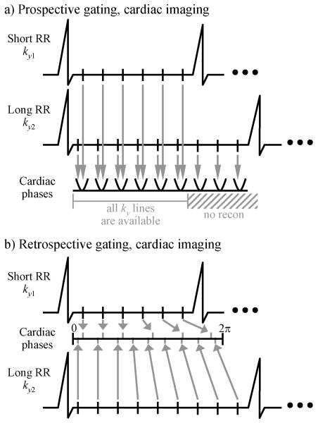
Figure 1 illustrates the main differences between prospective and retrospective gating. During a first heartbeat, a first set of k-space lines, which includes the line k_y1, gets sampled a number of times, at different cardiac phases. Each vertical black segment that intersects the ECG line, in-between consecutive R-waves, depicts one instance when k_y1 gets sampled. To keep the drawing visually simple, only 6 such instances were drawn, although a higher number of about 15 to 20 time samples might be acquired, for any given k-space line, in a typical cardiac scan.

Fig. 1.

While both prospective and retrospective cine imaging may be identical at the acquisition stage, they differ in the way the acquired data get mapped into cardiac phases. a) Any given k-space line is acquired at multiple time points during a cardiac cycle, and prospective gating involves a direct mapping, or binning, of these time points into cardiac phases. b) Retrospective gating on the other hand requires a temporal interpolation operation, as time points get converted into cardiac phases. Note that time samples are not necessarily mapped evenly onto the cardiacphase axis, as diastolic duration tends to be much more variable than systolic duration during arrhythmia.

During a second heartbeat, a second set of k-space lines gets sampled, which includes the line k_y2. Because the second heartbeat happens in this example to be significantly longer than the first one, more samples can be acquired for k_y2 during this second heartbeat than were acquired for k_y1 during the first heartbeat. The difference between prospective and retrospective gating, and thus the difference between Fig. 1a and 1b, comes from the way data get mapped onto a cardiac phase axis, at the reconstruction stage.

As depicted in Fig. 1a, prospective gating bins k-space lines according to the order in which they were acquired. Each cardiac phase can be seen as a bowl, or a bin, being filled with one copy of each k-space line (see vertical gray lines). While this strategy makes perfect sense at the beginning of the RR interval, the situation gets more complicated toward the end of the interval, during end-diastole, especially when significant arrhythmia is present. As depicted in Fig. 1a, the data acquired toward the end of the longer heartbeats cannot easily be reconstructed, because the k-space locations sampled during shorter heartbeats are missing, and accordingly, prospectively gated sequences tend to have difficulties capturing the end of the diastole.

Figure 1b represents the strategy employed in retrospective gating. All of the acquired data for any given line get distributed over a cardiac-phase axis ranging from 0 to 2π. Data from different heartbeats may fall at different locations along the cardiac phase axis, and for this reason, full k-space matrices cannot be readily assembled, at any cardiac phase. A temporal interpolation is required, to evaluate each one of the k-space lines at a common set of desired cardiac-phase locations. Once all k-space lines are made available through interpolation at a common set of cardiac-phase locations, these k-space lines are assembled into k-space matrices, and Fourier transformed to the object domain.

From Fig. 1b, note that regardless of the length of a heartbeat, all of the acquired data is readily used in the reconstruction, and that end-diastolic phases are captured. Both with prospective and retrospective gating, temporal interpolation is typically used to increase the number of reconstructed cardiac phases. But in prospective gating, temporal interpolation is just an optional step that could be performed at any stage of the reconstruction process, while in retrospective gating it is an essential step that must be performed at the beginning of the reconstruction process.

2. Temporal acceleration can readily be combined with prospective gating

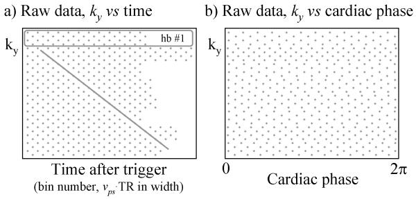
Figure 2a and 2b both depict the reconstruction of a same dataset, but Fig. 2a represents prospective gating while Fig. 2b represents retrospective gating. As can be seen in Fig. 2a, the sampling function gets shifted along k_y from one time point to the next, and less time points are acquired during shorter heartbeats (e.g., hb #1) than during longer ones. An increasingly large number of k-space locations are missing at later time points, making late-diastolic phases difficult to reconstruct (Fig. 2a). As can be seen from Fig. 2b, this problem is avoided with retrospective gating, and all cardiac phases can be reconstructed. The nice grid-like regularity of the k-t space data [14] depicted in Fig. 2a is, however, lost in Fig. 2b.

Fig. 2.

a) Using prospective cardiac gating, a k_y-t matrix can be built which features much regularity and simplicity. The UNFOLD sampling function is shifted from frame to frame, as highlighted by the oblique gray line. Data acquired during different heartbeats may feature different number of time samples, and the data acquired during the first heartbeat (hb) is highlighted by a gray rectangle. b) In retrospectively gated imaging however, the acquired data is distributed along a cardiac-phase axis, and much of the simplicity seen in (a) disappears in (b). A visual comparison of (a) and (b) makes it easier to understand why methods with time-variable sampling such as UNFOLD, TSENSE, UNFOLD-SENSE, k-t BLAST and k-t SENSE are more easily implemented on prospectively-gated sequences than retrospectively-gated ones.

With prospective gating, because k-space lines can readily be binned and grouped into time frames, UNFOLD can be applied essentially in the same way as in non-gated applications. Temporal interpolation, to increase the number of reconstructed time frames, does not interfere with the UNFOLD processing, and can be performed at the end, once the UNFOLD processing is finished. The more disorganized nature of the data in Fig. 2b, as compared to Fig. 2a, is the main reason why temporal acceleration schemes are more difficult to combine with retrospectively gated reconstructions than with prospectively gated ones.

3. Proposed approach for combining temporal acceleration with retrospective gating

The nice regularity of Fig. 2a, its ‘sheared-grid’ aspect, the ability to readily apply FFTs along all dimensions, all of these simple features disappear in Fig. 2b. One viable approach to combine temporal acceleration with retrospective gating involves treating the cardiac-phase axis as a non-Cartesian sampling problem, and numerically solving the resulting system of linear equations [8]. We show here instead that by carefully ordering the various processing steps involved to avoid the need for solving a large inverse problem, one can generate similar results in a much shorter time. The proposed algorithm is described below.

Overview of proposed algorithm

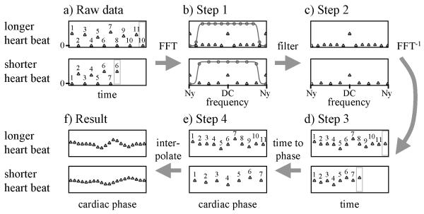
UNFOLD functions by densely packing information in x-y-f space. Such efficient packing may enable the suppression of artifacts that would otherwise have been left over by parallel imaging reconstructions [4, 6]. In one particular implementation presented in Ref. [9], UNFOLD was used along with the assumption that only part of the FOV is dynamic, while the rest of the FOV is nearly static (e.g., a beating heart surrounded by mostly-static thoracic tissues). It may be worth emphasizing that other applications, for example the fMRI UNFOLD application from Ref. [9], our prior work in [4, 6] as well as the work presented here, do not make such assumption, and that an entirely dynamic FOV could in principle be handled. Exactly as done in Refs [4, 6], artifact suppression is achieved here in two complementary ways. First, some artifacts are made to ‘flicker’ in time so they could readily be identified and filtered out. This step will be described in more details below, and in Fig. 3a-c. Secondly, artifacts are moved away from low temporal frequencies where the main bulk of the non-artifactual signal lies, allowing this crucial and signal-rich section of the temporal frequency domain to be reconstructed in a more reliable fashion, using a parallel imaging algorithm with reduced acceleration settings. As explained below, this step involves performing a second pass through the algorithm from Fig. 3. This second pass involves a narrower filter to select only the DC region, and a reduced parallel imaging acceleration factors. The algorithm proposed here is essentially equivalent to the one from Ref. [4], except that many of the processing steps previously performed in the image plane are now tailored instead to individual k-space points, to allow the retrospectively-gated reconstruction from Fig. 3d-f to be properly inserted into the reconstruction chain. While in most dynamic applications temporal processing could typically be performed equivalently well on k-space or image data, in contrast in retrospectively gated cine imaging a k-space processing proves necessary. In the explanations below, all processing steps are illustrated in Fig. 3 both for a long and for a short heartbeat, to illustrate how the approach handles arrhythmia. Every data point in Fig. 3 is complex, although only the magnitude is displayed.

Fig. 3.

This figure describes every step of the proposed processing. a-d) The UNFOLD filtering comes first, one k-space point at a time. As different number of time points were acquired at different k-space locations, the temporal filtering operation must be tailored to any given k-space location. e,f) The temporal interpolation required in retrospective-gating occurs next, finally followed by all needed spatial operations. See text for more details.

Step 1, A temporal FFT is applied to each k-point, individually (from Fig. 3a to 3b)

As typically done with UNFOLD, all missing data points are filled with zeros at the beginning of the processing. The data at each k-space location is Fourier transformed to the temporal frequency domain. Note that the number of time points may vary from one k-space location to another (because of arrhythmia), and accordingly the temporal FFT algorithm may have to process arrays of different lengths for different k-space locations. As usual with UNFOLD and related methods, one or more synthetic time frame(s) may have to be created before the temporal FFT is performed. This is because the FFT algorithm interprets the first and the last time points as being connected, and continuity in the time-varying sampling scheme must be ensured. For example, in Fig. 3a (top plot), a given k-space location is sampled on the first and every other odd time frame, but not on the second and every other even time frame, as the sampling function was shifted for these even time frames, and some other location got sampled instead. Note that there is an alternation between sampled and non-sampled points throughout the time axis, but that the first and last (11^th) time points are both sampled, breaking the alternation as the first and last points get connected. To ensure continuity, the frame before last is repeated at the end, into a synthetic time frame that will be cropped away once the UNFOLD processing is completed. It should be noted that the zeros in Fig. 3a have to do with spatial aliasing, not with temporal resolution. The sampling scheme is shifted from time frame to time frame, meaning that missing time points at one k-space location are actually available at neighboring k-space locations.

Step 2, A temporal-frequency filter is applied (from Fig. 3b to Fig. 3c)

Much of the artifact energy has been moved to the Nyquist frequency through the UNFOLD sampling scheme [9], and these artifacts are suppressed here with a filter (see peak at Nyquist in Fig. 3b). The same temporal-frequency filter (the gray curve shown in Fig. 3b) is applied to spectra obtained at all k-space locations. However, note that because different spectra may feature a different number of frequency points, the numerical values used in the actual filtering operation may differ. This point is illustrated in more detail in Fig. 3b. Both the data from a long heartbeat and a short heartbeat get filtered using the same filter, represented by a solid gray line. Because the temporal resolution in Fig. 3a was the same regardless of the length of the heartbeat, the Nyquist frequency, in Hz, has the same numerical value for short and long heartbeats, which justifies the use of the same filter in all cases. But as the distance between consecutive temporal-frequency points differs for long and short heartbeats, the filter gets evaluated at different frequency locations. Looking at the gray circles in Fig. 3b, notice that they all fall on the solid gray line of the filter, and that they are located at frequency locations where data are present. These circles represent the actual numerical values used in the filtering operation, and they differ for long and short heartbeats, as can be seen comparing the top and bottom parts of Fig. 3b.

Step 3, A temporal FFT⁻¹ is applied to each k-point, individually (from Fig. 3c to 3d)

Data is brought back to the time domain. Comparing the data in Fig. 3d to the raw data in Fig. 3a, note that the time points that were missing in the raw data have now been evaluated. For UNFOLD implementations where processing is performed in the spatial domain instead, this filling-in of missing k-space locations is replaced (equivalently) by a removal of aliasing artifacts. As described above, in the present application the processing must be performed before k-space matrices are assembled, and is thus performed on k-space points instead of image pixels.

Final steps, retrospective gating (from Fig. 3d to 3f)

The synthetic frame(s), if any, are no longer needed and are cropped away. The final steps, from Fig. 3d to 3e and then to 3f, correspond to a usual retrospectively gated reconstruction. Going from Fig. 3d to 3e, time frames are mapped onto a cardiac-phase axis, as also described in Figs 1b and 2b. Note that at this point, any desired non-linear mapping scheme could be employed. Because diastolic duration tends to be much more variable than systolic duration in the presence of arrhythmia, it is well known that non-linear mapping schemes may prove more physiologically correct. Finally, data from Fig. 3e are interpolated to a common set of cardiac-phase locations, regardless of the fact that different k-space locations may have been acquired during heartbeats of different durations. The steps from Fig. 3d to 3f are identical to a retrospectively gated reconstruction, and accordingly, they do not make any more or less assumptions about cardiac dynamics and repeatability than retrospective gating does. Once all k-space points are available at each desired cardiac phase, a spatial FFT algorithm produces the final result, a cardiac-phase series of images where aliasing artifacts have been suppressed.

Common variations on the algorithm proposed above

In our own work, even at high-acceleration settings, we prefer cycling through no more than 2 different variable-density sampling schemes to avoid creating ‘blind spots’ in the reconstructed bandwidth [15]. But in other implementations, one might decide instead to cycle through n different sampling patterns with an acceleration factor of n, returning to a given k-space location only once every n time frames. In such case, as many as n-1 synthetic frames may be required, to make the number of time frames a multiple of n, as depicted in Fig. 3a for the case n = 3. Furthermore, in some applications the last time frame may be very different from the first time frame, e.g., in dynamic enhancement applications where there is no contrast agent in the first frame and much enhancement in the last frame. In such applications, a larger number of synthetic frames may be required, to make the transition between last and first frames a smoother one. But in the present application, the motion is cyclical, as the heart should appear the same at phases 0 and 2π. Because of the cyclical nature of the imaged object, the simple scheme in Fig. 3a and 4a for generating synthetic frames proves appropriate.

Fig. 4.

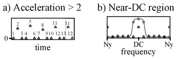
Variations on the scheme described in Fig. 3 may be applied. a) More ‘synthetic frames’ (highlighted in gray) may sometimes be used than shown in Fig. 3a. b) To extract near-DC information (either to generate sensitivity maps or as part of an artifact-suppression strategy), the processing may have to be repeated once or more times with filters of different bandwidths than the one in Fig. 3b. See text for more details.

While UNFOLD can be used by itself in cardiac imaging, a preferred implementation involves using it in combination with parallel imaging. Doing so requires a second pass through the algorithm in Fig. 3, as described in more details below.

4. Combining the approach with parallel imaging

Ordering of the operations

Parallel imaging employs a spatially based encoding, and cannot be performed until all appropriate spatial frequency points or spatial pixels are combined at a given cardiac phase. In other words, parallel imaging should be performed after the temporal interpolation, which evaluates all spatial information at a common set of cardiac phases. While typically one has the choice of applying the temporal UNFOLD processing either before or after the parallel-imaging reconstruction, this choice disappears here, and UNFOLD is performed first. Except for this small difference, the extension of the present approach to methods like TSENSE or UNFOLD-SENSE is mostly straightforward.

Two separate passes through the algorithm from Fig. 3

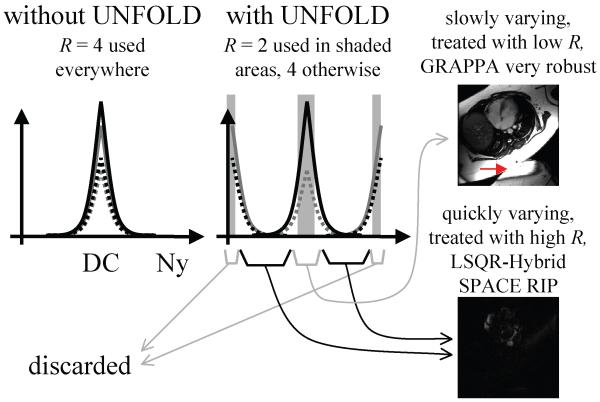
The effect of UNFOLD’s time-variable sampling is to displace signals that correspond to aliased material to benign locations on the temporal frequency axis. Moving half the overlapped components all the way to the Nyquist frequency and keeping the other half near DC creates a narrow frequency region near DC, shown shaded in Fig. 5, where the aliasing problem has been partly resolved. Because only half the components have significant signal at DC, the parallel-imaging acceleration factor can be halved when reconstructing the temporal DC region [4, 6]. The algorithm from Fig. 3 is run twice on the acquired data: once with a narrow filter (FWHM 10% of the bandwidth) in Fig. 3b, to isolate the near DC signals, and once with a wider filter (FWHM 90% of the bandwidth). The latter pass leads to signals that can be reconstructed with a parallel imaging acceleration factor R, while the former leads to near-DC signals that can be reconstructed with a parallel imaging factor R/2. Appropriate filters are then used to combine results from both passes [4, 6].

Fig. 5.

The main effect of time-variable sampling is to move aliased components to benign locations on the temporal frequency axis, creating regions (shown shaded here) where the overlap problem has been alleviated. Accordingly, a lower acceleration factor can be used near DC as compared to the rest of the bandwidth. Because imaged objects tend to have their full spatial extent at the DC temporal frequency, unintended spatial overlaps (see red arrow) can be considered more likely at low temporal frequencies. In contrast, quickly varying signals tend to appear mostly near the outline of the heart, and unintended spatial overlaps are thus not likely at high temporal frequencies. For these reasons we use GRAPPA, well-known for its robustness in the presence of such unintended overlaps, to reconstruct the near DC signal at lower acceleration factors, while the SPACERIP method is used to reconstruct higher frequency signals given its better regularization flexibility.

Combining the strengths of GRAPPA and SPACERIP

The proposed processing involves using at least two different parallel imaging reconstructions for at least two different temporal frequency bands. While these reconstructions may differ only in terms of acceleration factor (e.g., a SENSE R=4 reconstruction for high temporal frequencies and a SENSE R=2 for the DC region), one might very well further change the actual method employed. In the present implementation, through experience, we came to consider a combination of GRAPPA and SPACERIP as our preferred implementation. Figure 5 helps explain the strengths of this particular combination. In cases where the FOV is erroneously set too small for the imaged anatomy, signal overlap may still be present in the final de-aliased images (e.g., see red arrow in Fig. 5). As shown in Fig. 5, such overlap is much more likely in images near the DC temporal frequency, where the object typically appears in its full spatial extent, than in images from higher temporal frequencies where only the outline of the heart itself and a few vessels may be clearly visible. Robustness in the presence of such overlap is a well-known strength of GRAPPA, unlike the SENSE or SPACERIP methods. On the other hand, SPACERIP provides a solution that minimizes the least-mean-squared error and offers more flexibility in terms of regularization than GRAPPA, which may be an advantage at high acceleration settings. In our experience, noise amplification at high acceleration could be better kept under control with our SPACERIP than with our GRAPPA algorithm. Accordingly, it appeared natural to use GRAPPA when the risk for overlap is high (i.e., when reconstructing near-DC signals with lower acceleration values), and SPACERIP when the risk for overlap is low (higher frequencies at higher acceleration values). Here, we use GRAPPA to reconstruct the results from a first pass through the algorithm from Fig. 3, with narrow filter in Fig. 3b, SPACERIP is used to reconstruct the output of the second pass, with a wider filter (Fig. 3b).

5. Description of the implementation

The proposed approach was implemented on a 1.5 T and a 3T system (software release 14; GE Medical Systems, Milwaukee, WI, USA) using product GE eight-element cardiac phased-array coils. Written informed consent was obtained from all participants, and the associated protocol was approved by our Institutional Review Board (IRB). A modified version of a cardiac-gated steady-state free precession (SSFP) sequence was used, along with GE’s raw data server (RDS) software. Because the raw data obtained using the RDS software does not feature any header information, code was added to the pulse sequence to open a separate file and store scan and sampling function information. A third file was generated immediately following the data acquisition, to store information regarding the exact timing of the R-waves. Reconstruction does not require any user interaction, and does not involve any parameter adjustment or tweaking of any kind from patient to patient.

The reconstruction was performed with programs written in the C language, and employed functions from the Fast Imaging Library developed within our group. This library and associated documentation are freely downloadable from the National Center for Image-Guided Therapy site (www.ncigt.org/pages/Research_Projects/ImagingCoreToolbox/Imaging_Toolkit). Data from seven patients and one healthy volunteer were acquired, and results from all these consecutive cases are shown here. There were no particular inclusion criteria beyond being scheduled for a Cardiovascular Magnetic Resonance (CMR) study at our institution, for the patient scans. Informed consent was obtained shortly before the scans.

A variable density k-space sampling pattern was used, whereby the reduction factor was equal to 4 in the outer regions of k-space and equal to 2 in the DC region (as described in the self, hybrid referencing with UNFOLD and GRAPPA (SHRUG) method [6]). The composite acceleration was thus either 3.5 without partial-Fourier (55 k_y lines instead of 192), or 4.5 with partial-Fourier (43 lines instead of 192). As compared to our clinical protocol, the acceleration was used in the patient scans to reduce the number of heartbeats required to generate images, i.e., to reduce breath-hold duration.

As shown in Fig. 5, different parallel imaging algorithms can be used for low temporal frequencies than for higher temporal frequencies. Our implementation handled all possible combinations of Cartesian SENSE, GRAPPA and SPACERIP for these two separate reconstructions. Through experience, our preferred combination involves using GRAPPA at a lower acceleration factor near DC and SPACERIP at a higher acceleration factor in the rest of the reconstructed bandwidth. Note that GRAPPA could not readily be used for the higher-acceleration reconstruction, as no fully-sampled central k-space region would be available to calculate GRAPPA coefficients from. The six tested combinations were thus: SENSE-SENSE, SPACERIP-SPACERIP, SENSE-SPACERIP, SPACERIP-SENSE, GRAPPA-SPACERIP and GRAPPA-SENSE, with the GRAPPA-SPACERIP case emerging as our preferred implementation. All scaling issues had to be carefully resolved between our GRAPPA, SPACERIP and Cartesian SENSE software, so their outputs might be compatible for all possible choices of imaging parameters. For the SPACERIP implementation, a higher-acceleration reconstruction was performed by feeding odd and even k-lines separately. Indeed, the UNFOLD part of the algorithm populates with data some k-space locations that were not actually sampled (e.g., compare Fig. 3a and 3d), and feeding all k-space lines together into a SPACERIP implementation would be interpreted by the algorithm as a lower-acceleration reconstruction. By simply feeding odd and even lines separately, and then adding the results, one obtains the desired higher-acceleration reconstructions. The SPACERIP implementation employed a Tikhonov regularization term, with automatic adjustment of the regularization parameter. Multiple solutions were found via an efficient least-squares (LSQR-Hybrid [16]) numerical solver. This solver generates multiple solutions, for different settings of the regularization parameter, at a computing cost only marginally greater than that of a single solution, for a single regularization setting. From these multiple solutions, an appropriate value for the regularization parameter can be identified, which provides the best noise suppression without adversely affecting image details. This selection process is based on quality metrics that typically involve L-curve or discrepancy methods (the discrepancy method was used here). An appropriate Tikhonov parameter value was selected in this manner, independently for each slice, using data from the first cardiac phase. The same regularization setting was then used for all subsequent cardiac phases.

Results

1. Clinical significance

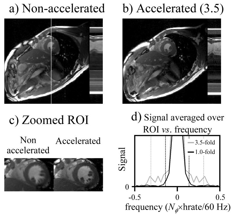
Figure 6 shows non-accelerated and accelerated results obtained in a healthy volunteer at 3 T (heart rate = 61 bpm, FOV = 32×32 cm, matrix size = 192×192, slice thickness = 8 mm, bandwidth = 125 kHz, TR = 3.8 ms, TE = 1.7 ms, and number of k_y lines per heartbeat = 12 or 30, for accelerated and non-accelerated cases, respectively). While the nominal acceleration factor was 3.5, it is convenient to define an “effective acceleration” factor that includes the smoothing effect of the UNFOLD filter from Fig. 3b. Because 10% of the temporal bandwidth is sacrificed toward suppressing aliasing artifacts, the effective acceleration factor here was 0.9×3.5 = 3.15. As compared to the non-accelerated case, acceleration was used to roughly double temporal resolution (from 30×TR to 12×TR/0.9), and to slightly reduce scan time (from 7 to 5 hb).

Fig. 6.

Non-accelerated (a) and accelerated (b) results are compared, where most of the acceleration was used to increase temporal resolution. While a mid-systolic phase is show in (a) and (b), an early-systolic phase is shown instead in (c). The temporal frequency content for the ROI in (c) is plotted in (d), confirming that as expected, the accelerated results (3.5-fold) feature signal over a frequency range about twice as wide as the non-accelerated results (1.0-fold).

As demonstrated here, one clinically useful application of the proposed method involves using it to achieve at once both a good temporal resolution and a short scan time, without having to sacrifice one for the other. As compared to accelerated applications based on parallel imaging only, the present method allows better image quality to be maintained at higher acceleration settings (as demonstrated in section 2, below). The fact that the accelerated results have better temporal resolution can readily be seen from Fig. 6a-c, and is tested more quantitatively in Fig. 6d. The (magnitude) results were FFTed along the cardiac phase axis, and summed over the spatial ROI from Fig. 6c, to show the temporal frequency content for both accelerated and non-accelerated reconstructions (Fig. 6d). Even though a same number of cardiac phases were reconstructed for both datasets (N_φ = 30), the non-accelerated case is expected to actually feature only about half the range of temporal frequencies captured in the accelerated case, more specifically, 1/(30×TR) Hz compared to 0.9/(12×TR) Hz, with TR expressed in s. These expected ranges are shown in Fig. 6 using vertical dashed lines. From Fig. 6d, please note that all of the claimed temporal resolution does seem to indeed be present in the final reconstructed results (i.e., looking at the gray curve in Fig. 6d, it features significant signal all the way to both gray dashed vertical lines).

2. Patient results

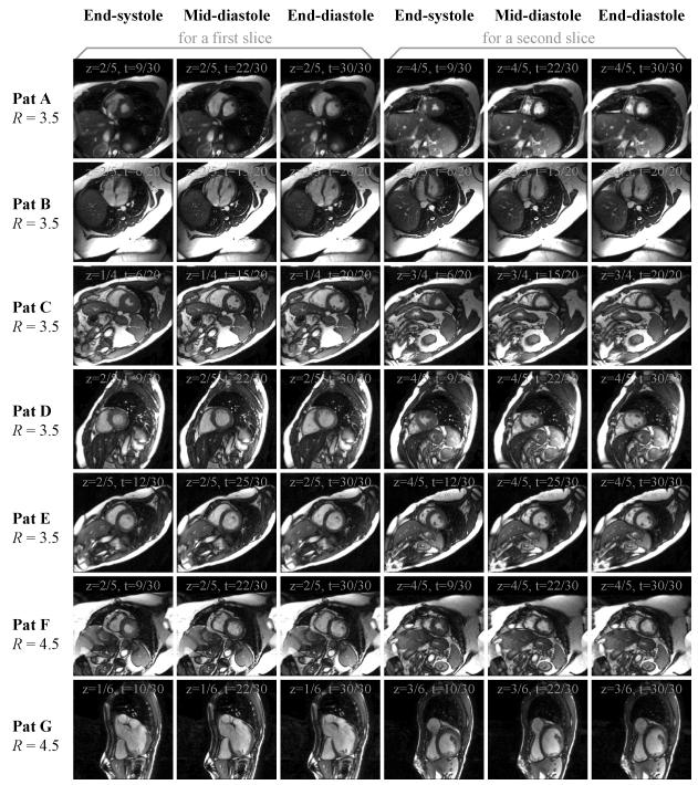
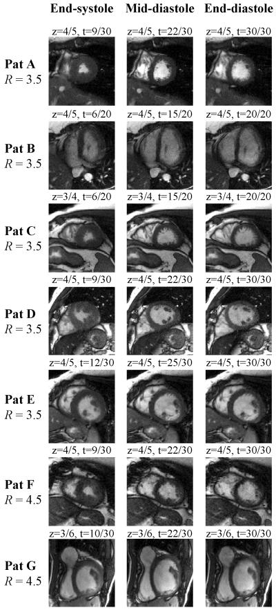
Results from all seven patients are shown in Fig. 7, in the chronological order in which they were acquired. Results are shown at 3 different cardiac phases (end-systole, mid-diastole, end-diastole), for 2 different slices. Phases and slices not shown here were of quality equivalent to those displayed in Fig. 7. The full FOV was erroneously set to values slightly smaller than the imaged anatomy in 3 patients (A, B and F), and patient B presented severe cardiac irregularity (bigemini condition). Imaging parameters are listed in Table 1, and include the number of k_y lines per heartbeat (sometimes called ‘views-per-segment’), matrix size, slice thickness, number of slices acquired, acceleration factor R, number of heartbeats required to image one slice, and the heart rate in beats per minute (bpm). The number of heartbeats is given by the number of k_y lines divided by the number of views per segment (vps) and by the acceleration factor: # of beats = ceil(192 / (R × vps)). A zoom over the heart region is shown in Fig. 8 for each patient, for one of the two slices from Fig. 7.

Fig. 7.

Results from all 7 patients are shown here, for two slices ‘z’ and three cardiac phases ‘t’. Note that reasonable image quality was obtained in all cases, even though the FOV was set slightly too small for patients A, B and F. Slices and phases not shown here were of similar quality to those displayed.

Table 1.

Scan parameters and LV measurements

Patient	Ejection fraction	Atrial booster	Views per segment	Matrix size	Slice (mm)	# of slices	R	# of beats	Heart rate (bpm)
A	64%	13%	12	192x 192	8	5	3.5	5	58
B	43%	5.4%	12	192x 192	8	5	3.5	5	64
C	71%	15%	10	192x 192	8	4	3.5	6	63
D	61%	13%	12	192x 192	8	5	3.5	5	-
E	31%	3.6%	10	192x 192	8	5	3.5	6	104
F	69%	18%	12	192x 192	8	5	4.5	4	58
G	31%	3.7%	10	192x 192	8	6	4.5	5	75

Fig. 8.

Images from Fig. 7 were zoomed to better show the heart region. Differences between the mid-diastolic and end-diastolic images confirm that the present retrospectively gated method appears to correctly capture the end-diastolic phase, when the left atrium contracts and gives a boost in volume to the left ventricle, just before ventricular systole.

Reconstruction time on a single processor of a single 2.4 GHz PC was 0.98±0.07 s per frame, and memory usage was modest, below 500 MB in all cases. The number of reconstructed frames is a free parameter in retrospectively gated reconstructions, and some datasets were reconstructed here with 20 frames (patients B and C) while all others were reconstructed with 30 frames. Accordingly, at about 1 s per frame, each slice from patient B and C took about 20 s to reconstruct, and about 30 s for the other patients, for an overall reconstruction time of 26.5±3.6 s per slice. Replacing GRAPPA and SPACERIP by variable-density Cartesian SENSE gives about a two-fold reduction in reconstruction time (12.3±1.2 s per slice). Despite longer reconstruction times, the more robust implementation based on GRAPPA and SPACERIP is recommended here over that based on Cartesian SENSE. Although faster, reconstructions based on Cartesian SENSE were associated with higher artifact content.

The area of the left ventricle was evaluated at the three phases shown in Fig. 7 and 8, for all acquired slices. These values were used to approximate the end-systolic volume (ESV), mid-diastolic volume (MDV) and end-diastolic volume (EDV). Approximations for the ejection fraction (EDV-ESV)/EDV and the atrial booster (EDV-MDV)/EDV are listed in Table 1. Please note that these values are not necessarily expected to be accurate, as the number of imaged slices in the research scans was insufficient to appropriately cover the ventricle. The number of imaged slices was kept low (5 on average) to make the addition of a research study more readily acceptable to clinicians, technologists and patients. Important results here are the atrial booster values, which suggest the proposed approach appropriately captures the end-diastolic phase, when the atrium contracts to give a boost in volume to the ventricle. Atrial booster values around 15% are typically considered normal, and similar values were found in all patients except patient B (bigemini condition), patient E (pericardial constriction) and patient G (cardiomyopathy).

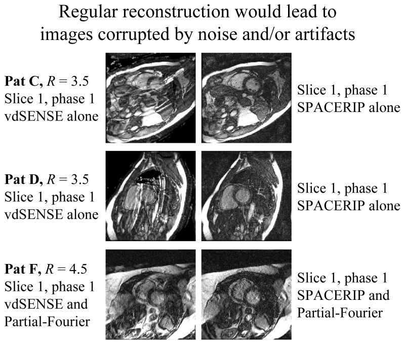
As shown in Fig. 9, regular reconstructions using parallel imaging without UNFOLD would not lead to satisfactory results here. While better phased-array coils with more elements might be capable of supporting parallel-imaging accelerations of 3.5 or 4.5, such acceleration factors were beyond the capabilities of the phased-array coil we were using. Results are shown in Fig. 9 for two different parallel imaging methods, vdSENSE and SPACERIP. The difference between results from these two methods has much more to do with the regularization method used in the respective implementations than with the actual methods themselves. While the regularization used in the SPACERIP implementation tended to suppress aliasing artifacts at a price in noise and blurring, the regularization used in vdSENSE mostly avoids noise amplification and blurring at a price in artifacts. The main message from Fig. 9 is that for the datasets presented in Fig. 7, a regular reconstruction would not have been a viable alternative. For a given coil array, our proposed algorithm allows greater image quality at greater acceleration to be achieved, as compared to using parallel imaging without UNFOLD.

Fig. 9.

As can be seen comparing these images with their counterparts from Fig. 7, regular reconstructions with parallel imaging but without UNFOLD would not have been a viable option. Parallel-imaging acceleration factors of 3.5 (without partial-Fourier) or 4.5 (with partial-Fourier) were beyond the abilities of our product phased-array coil. Differences between vdSENSE results and SPACERIP results are mostly due to regularization. Notice that when including UNFOLD, and as shown in Fig. 7, good-quality results were obtained instead.

3. Comparisons with prior work

Comparisons between the proposed algorithm and previously published work involved volunteer data and programs written in the Matlab language (The MathWorks, Natick, MA, USA). To make the compared methods more equivalent, similar regularization schemes were selected. For these comparisons, the proposed approach employed the regularization scheme described in k-t SENSE [5], which uses prior knowledge to identify a diagonal regularization operator (as opposed to just a scalar in zero-order Tikhonov regularization). Furthermore, coil sensitivity information was included into the encoding matrix in our implementation of the retrospectively-gated accelerated work from Hansen et al [8], so that both compared methods equivalently included a parallel imaging component. Note that because the method from Hansen et al requires a conjugate solution in one more dimension than our proposed method (2D instead of 1D), longer reconstruction times should be expected.

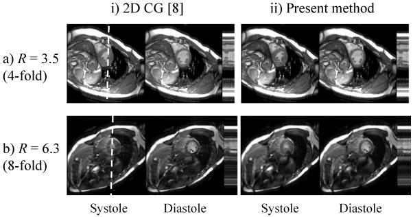
Comparisons were performed between the proposed algorithm and that from Hansen et al [8] and results are presented in Fig. 10 (acceleration factor of 3.5 obtained by selecting one line every 4, and factor 6.3 by selecting one line very 8, plus extra lines near center). We made a version of our proposed method in the Matlab language, associated with reconstruction times about an order of magnitude slower than our C implementation. The fast C implementation of our method was not used in the comparison, but rather our slower Matlab implementation, to make the compared implementations more equivalent. The method from [8] was also implemented in the Matlab language, and featured reconstruction times about 8 times longer than the Matlab implementation of our method. Similar image quality was obtained in both cases. While processing times are of course highly dependant on code optimization and programmer skills, efforts were made to make both implementations reasonably efficient. Maybe more importantly, the theory of the methods involved strongly suggest our implementation should indeed be significantly faster, as it involves 1D conjugate gradient solutions (along k_y, as part of SPACERIP) rather than 2D conjugate gradient solutions (along both k_y and time axes). For this reason, the present results merely confirm what might have reasonably been expected, that 2D conjugate gradient solutions typically take longer than 1D conjugate gradient solutions. Acquisitions were truly accelerated by a factor of R, and accordingly no fully sampled ‘truth’ is available for comparison.

Fig. 10.

Volunteer datasets were reconstructed using both the proposed method and that from [8], with acceleration factors of 3.5 (skip factor of 4 in k-space) and 6.3 (skip factor of 8). We included sensitivity information into the encoding matrix for our implementation of the retrospectively-gated accelerated method from [8], and as a consequence both compared methods employed parallel imaging. While no significant differences were observed in terms of image quality, the present algorithm had a processing time several-fold shorter. Using a Matlab implementation for both methods, reconstruction time using the proposed approach was about 8 times faster.

Discussion and Conclusion

A robust and practical method for faster retrospectively gated cardiac cine imaging was presented that achieves meaningful acceleration factors and clinically acceptable reconstruction times on readily available hardware. By breaking up the reconstruction problem into manageable steps, reconstruction time can be reduced by roughly an order of magnitude over alternative approaches, at little to no cost in image quality. A seven-patient study was presented to test the proposed method’s ability to provide interesting acceleration factors on commonly available hardware, for faster retrospectively gated cardiac cine imaging. The study featured some challenging cases, with slightly-too-small FOV values and/or significant arrhythmia. Image quality was considered excellent by collaborating cardiologists. Reconstruction time was very practical, at 0.98±0.07 s per frame on a 2.4 GHz PC.

The present approach assumes that the filtering step in the reconstruction (Fig. 3b) does not eliminate important heartbeat-related information. Risks are minimized here by using wide low-pass filters, with a FWHM equal to 90% of the bandwidth. While treating the effects of time-variable sampling and cardiac motion all at once as in [8] rather than sequentially may provide an advantage in terms of discriminating between the two effects, such advantage may come at the price of possible noise amplification, and possible losses in accuracy as regularization is employed to keep noise amplification under check. It may be useful to keep in mind that there is no such thing as an exact retrospectively gated reconstruction, as the idea that missing cardiac phases can be obtained by interpolating sampled ones is in itself an approximation, and further assumptions are required regarding cardiac repeatability and the effects of arrhythmia. Very much like retrospective gating itself, the present method is not meant as an exact solution to an exact problem, but rather as a practical solution to a practical problem, capable of generating clinically useful results in a reliable manner.

List of abbreviations

GRAPPA

generalized autocalibrating partially parallel acquisitions

k-t BLAST

k-t broad-use linear acquisition speed-up technique

SENSE

sensitivity encoding

SPACERIP

Sensitivity profiles from an array of coils for encoding and reconstruction in parallel

TSENSE

temporal SENSE

UNFOLD

unaliasing by Fourier-encoding the overlaps using the temporal dimension

References

- 1.Pruessmann KP, Weiger M, Scheidegger MB, Boesiger P. SENSE: sensitivity encoding for fast MRI. Magn Reson Med. 1999;42:952–962. [PubMed] [Google Scholar]
- 2.Griswold MA, Jakob PM, Heidemann RM, Nittka M, Jellus V, Wang J, Kiefer B, Haase A. Generalized autocalibrating partially parallel acquisitions (GRAPPA) Magn Reson Med. 2002;47:1202–10. doi: 10.1002/mrm.10171. [DOI] [PubMed] [Google Scholar]
- 3.Kellman P, Epstein FH, McVeigh ER. Adaptive sensitivity encoding incorporating temporal filtering (TSENSE) Magn Reson Med. 2001;45:846–852. doi: 10.1002/mrm.1113. [DOI] [PubMed] [Google Scholar]
- 4.Madore B. Using UNFOLD to remove artifacts in parallel imaging and in partial-Fourier imaging. Magn Reson Med. 2002;48:493–501. doi: 10.1002/mrm.10229. [DOI] [PubMed] [Google Scholar]
- 5.Tsao J, Boesiger P, Pruessmann KP. k-t BLAST and k-t SENSE: dynamic MRI with high frame rate exploiting spatiotemporal correlations. Magn Reson Med. 2003;50:1031–42. doi: 10.1002/mrm.10611. [DOI] [PubMed] [Google Scholar]
- 6.Madore B. UNFOLD-SENSE: a parallel MRI method with self-calibration and artifact suppression. Magn Reson Med. 2004;52:310–20. doi: 10.1002/mrm.20133. [DOI] [PubMed] [Google Scholar]
- 7.Kozerke S, Plein S. Accelerated CMR using zonal, parallel and prior knowledge driven imaging methods. Journal of Cardiovascular Magnetic Resonance. 2008;10:1–18. doi: 10.1186/1532-429X-10-29. [DOI] [PMC free article] [PubMed] [Google Scholar]
- 8.Hansen MS, Baltes C, Tsao J, Kozerke S, Pruessmann KP, Eggers H. k-t BLAST reconstruction from non-Cartesian k-t space sampling. Magn Reson Med. 2006;55:85–91. doi: 10.1002/mrm.20734. [DOI] [PubMed] [Google Scholar]
- 9.Madore B, Glover GH, Pelc NJ. Unaliasing by Fourier-encoding the overlaps using the temporal dimension (UNFOLD), applied to cardiac imaging and fMRI. Magn Reson Med. 1999;42:813–828. doi: 10.1002/(sici)1522-2594(199911)42:5<813::aid-mrm1>3.0.co;2-s. [DOI] [PubMed] [Google Scholar]
- 10.Utz JA, Herfkens RJ, Heinsimer JA, Bashore T, Califf R, Glover G, Pelc N, Shimakawa A. Cine MR determination of left ventricular ejection fraction. Am J Roentgenol. 1987;148:839–43. doi: 10.2214/ajr.148.5.839. [DOI] [PubMed] [Google Scholar]
- 11.Lenz GW, Haacke EM, White RD. Retrospective cardiac gating: a review of technical aspects and future directions. Magn Reson Imaging. 1989;7:445–55. doi: 10.1016/0730-725x(89)90399-8. [DOI] [PubMed] [Google Scholar]
- 12.Atkinson DJ, Edelman RR. Cineangiography of the heart in a single breath hold with a segmented TurboFLASH sequence. Radiology. 1991;178:357–360. doi: 10.1148/radiology.178.2.1987592. [DOI] [PubMed] [Google Scholar]
- 13.Chao T, Chung H, Hoge W, Yuan J, Madore B. 2D graphical assessment for fast imaging strategies: ISMRM. Honolulu; Hawai’i, USA: 2009. p. 2837. [Google Scholar]
- 14.Xiang QS, Henkelman RM. K-space description for MR imaging of dynamic objects. Magn Reson Med. 1993;29:422–8. doi: 10.1002/mrm.1910290324. [DOI] [PubMed] [Google Scholar]
- 15.Chao TC, Chung HW, Hoge WS, Madore B. A 2D MTF approach to evaluate and guide dynamic imaging developments. Magn Reson Med. 2010;63:407–18. doi: 10.1002/mrm.22219. [DOI] [PMC free article] [PubMed] [Google Scholar]
- 16.Hoge WS, Kilmer ME, Haker SJ, Brooks DH, Kyriakos WE. Fast regularized reconstruction of non-uniformly subsampled parallel MRI data: IEEE Intl Symp on Biomedical Imaging; Arlington, VA, USA. 2006.pp. 714–717. [Google Scholar]