On the C-statistics for Evaluating Overall Adequacy of Risk Prediction Procedures with Censored Survival Data

Abstract

For modern evidence-based medicine, a well thought-out risk scoring system for predicting the occurrence of a clinical event plays an important role in selecting prevention and treatment strategies. Such an index system is often established based on the subject’s “baseline” genetic or clinical markers via a working parametric or semi-parametric model. To evaluate the adequacy of such a system, C-statistics are routinely used in the medical literature to quantify the capacity of the estimated risk score in discriminating among subjects with different event times. The C-statistic provides a global assessment of a fitted survival model for the continuous event time rather than focuses on the prediction of t-year survival for a fixed time. When the event time is possibly censored, however, the population parameters corresponding to the commonly used C-statistics may depend on the study-specific censoring distribution. In this article, we present a simple C-statistic without this shortcoming. The new procedure consistently estimates a conventional concordance measure which is free of censoring. We provide a large sample approximation to the distribution of this estimator for making inferences about the concordance measure. Results from numerical studies suggest that the new procedure performs well in finite sample.

1. INTRODUCTION

For modern clinical medicine, risk prediction procedures are valuable tools for disease prevention and management. Pioneered by the Framingham study, risk score systems have been established for assessing individual risks of developing cardiovascular diseases, cancer or many other conditions within a certain time period [1, 2, 3, 4]. A key component in the assessment of risk algorithm performance is its ability to distinguish subjects who will develop an event (“cases”) from those who will not (“controls”). This concept, known as discrimination, has been well studied and quantified for binary outcomes using measures such as the estimated area under the Receiver Operating Characteristics (ROC) curve (AUC), which is also referred to as a “C-statistic” [5]. Such a statistic is an estimated conditional probability that for any pair of “case” and “control,” the predicted risk of an event is higher for the “case” [6].

If the primary response variable is the time to a certain event, the aforementioned procedure for binary outcomes can be used to quantify the ability of the risk score system to differentiate cases from controls at a time point t. If one is not interested in a particular time point, a standard concordance measure may be used to evaluate the overall performance of the risk scoring system. Specifically, let T be the event time, Z be a p × 1 covariate vector, and g(Z) be an estimated risk score for subjects with Z. There is a large class of measures to quantify how well the risk score g(Z) predicts the distribution of T or a function thereof. A good review paper is given by Korn & Simon [7] or more recently by Hielscher et al. [8] Such prediction measures can be classified into two broad classes, one based on explicit loss functions between the risk score and the survival time and the other based on rank correlations between these two quantities. The C-statistic proposed by Harrell et al. [9, 10, 11] is essentially a rank-correlation measure, motivated by Kendall’s tau for censored survival data [12]. A critical issue for rank correlation methods is how to order survival times in the presence of censoring. Brown et al. [12] used all observations and assigned probability scores to pairs in which ordering is not obvious due to censoring, based on the pooled Kaplan-Meier estimate for T. However, the score based on the pooled Kaplan-Meier estimate may not be appropriate when the covariates are associated with T. Alternative forms of C-statistic considered in [9, 10, 11, 13] use only so-called “useable” pairs and calculate the proportion of concordant pairs among them. However, such C-statistics estimate population parameters that may depend on the current study-specific censoring distribution. In this article, we propose a modified C-statistic which is consistent for a population concordance measure that is free of censoring.

More specifically, for two independent copies {(T₁, g(Z₁))′, (T₂, g(Z₂))′} of (T, g(Z))′, a commonly used concordance measure is

$$C=\mathrm{pr}(g(Z_1)>g(Z_2)\mid T_2>T_1)$$ (1.1)

[14]. When T is subject to right censoring, as discussed in Heagerty & Zheng [14] one would typically consider a modified C_τ with a fixed, prespecified follow-up period (0, τ), where

$$C_{\tau }=\mathrm{pr}(g(Z_1)>g(Z_2)\mid T_2>T_1,T_1<\tau ).$$ (1.2)

Estimation of (1.1) or (1.2) when the event time may be censored, however, is not straightforward [11, 13, 15]. The estimator for C or C_τ proposed by Heagerty & Zheng [14] is derived under a proportional hazards model. If this semi-parametric working model is not correctly specified, the resulting estimator may be biased. A popular nonparametric C-statistic for estimating C or C_τ was proposed by Harrell et al. [9, 10, 11] and extensively studied by Pencina & D’Agostino [13]. Note that this generalization is a weighted area under an “incident/dynamic” ROC curve [14, 16] with weights depending on the study-specific censoring distribution.

When the study individuals have different follow-up times, the C-statistic studied by Harrell et al. [9, 10, 11] converges to an association measure that involves the study censoring distribution. In this article, under the general random censorship assumption, we provide a simple non-parametric estimator for the concordance measure in (1.2), which is free of censoring. Furthermore, we study the large sample properties of the new estimation procedure. Our proposal is illustrated with two real examples. The performance of the new proposal under various practical settings is also examined via a simulation study. Note that Gönen & Heller [17] proposed a method for censored survival data to estimate pr(T₂ > T₁ ∣ g(Z₁) > g(Z₂)), which is also a concordance measure and has a similar form to (1.1), but we do not focus on this type of measures in this paper.

2. INFERENCE PROCEDURES FOR DEGREE OF ASSOCIATION BETWEEN EVENT TIMES AND ESTIMATED RISK SCORES

In this section, we consider a non-trivial case that at least one component of the covariate vector Z is continuous. For the survival time T, let D be the corresponding censoring variable. Assume that D is independent of T and Z. Let {(T_i, Z_i, D_i), i = 1, …, n} be n independent copies of {(T,Z,D)}. For the ith subject, we only observe (X_i, Z_i, Δ_i), where X_i = min (T_i, D_i), and Δ_i equals 1 if X_i = T_i and 0 otherwise.

Suppose that we fit the data with a working parametric or semi-parametric regression model, for example, a standard Cox proportional hazards model [18]:

$${\mathrm{\Lambda }}_Z(t)={\mathrm{\Lambda }}_0(t)\exp ({\beta }^{\prime }Z),$$ (2.1)

where Λ_Z(·) is the cumulative hazard function for subjects with covariate vector Z, Λ₀(·) is the unknown baseline cumulative hazard function and β is the unknown p × 1 parameter vector. Let the maximum partial likelihood estimator for β be denoted by β̂. Note that even when the model (2.1) is not correctly specified, under a rather mild non-separable condition that there does not exist vector ζ such that pr(T₁ > T₂ ∣ ζ′Z₁ < ζ′Z₂) = 1, β̂ converges to a constant vector, say, β₀, as n → ∞. This stability property is important for deriving the new inference procedure.

For a pair of future patients with covariate vectors $\{Z_k^0,k=1,2\}$ and the potential survival times $\{T_k^0,k=1,2\}$, their corresponding risk scores are $\{{\widehat{\beta }}^{\prime }{Z}_k^0,k=1,2\}$. To evaluate this risk score system, one may use the concordance measure discussed in Section 1:

$$C_n=\mathrm{pr}({\widehat{\beta }}^{\prime }{Z}_1^0>{\widehat{\beta }}^{\prime }{Z}_2^0\mid T_1^0<T_2^0),$$

where the probability is evaluated with respect to the data, and ( $T_1^0,Z_1^0$) and ( $T_2^0,Z_2^0$). Note that C_n depends on the sample size. Let the limit of C_n be denoted by

$$C=\mathrm{pr}({\beta }_0^{\prime }{Z}_1^0>{\beta }_0^{\prime }{Z}_2^0\mid T_1^0<T_2^0).$$ (2.2)

Now, since the support of the censoring variable D is usually shorter than that of the failure time T, the tail part of the estimated survival function of T is rather unstable. Therefore, we consider a truncated version of C in (2.2), that is,

$$C_{\tau }=\mathrm{pr}({\beta }_0^{\prime }{Z}_1^0>{\beta }_0^{\prime }{Z}_2^0\mid T_1^0<T_2^0,T_1^0<\tau ),$$ (2.3)

where τ is a prespecified time point such that pr(D > τ) > 0.

It follows from an “inverse probability weighting” technique as employed in Cheng et al. [19] for dealing with a completely different problem in survival analysis that C_τ can be consistently, nonparametrically estimated by

$${\widehat{C}}_{\tau }=\frac{{\sum }_{i=1}^n{\sum }_{j=1}^n{\mathrm{\Delta }}_i{\{\widehat{G}(X_i)\}}^{-2}I(X_i<X_j,X_i<\tau )I({\widehat{\beta }}^{\prime }{Z}_i>{\widehat{\beta }}^{\prime }{Z}_j)}{{\sum }_{i=1}^n{\sum }_{j=1}^n{\mathrm{\Delta }}_i{\{\widehat{G}(X_i)\}}^{-2}I(X_i<X_j,X_i<\tau )},$$ (2.4)

where I(·) is the indicator function and Ĝ(·) is the Kaplan-Meier estimator for the censoring distribution G(t) = pr(D > t). Heuristically, the consistency of the above estimator follows from the fact that as n → ∞, the denominator of (2.4) divided by n² converges to

$$\begin{array}{lll}E\left\{{\mathrm{\Delta }}_1{\left\{G\left(X_1\right)\right\}}^{-2}I\left(X_1<X_2,X_1<\tau \right)\right\}& =& E\left[E\left\{I\left(D_1\wedge D_2>T_1\right){\left\{G\left(T_1\right)\right\}}^{-2}I\left(T_1<T_2,T_1<\tau \right)\mid T_1\right\}\right]\\ & =& E\left[E\left\{I\left(D_1>T_1\right)I\left(D_2>T_1\right){\left\{G\left(T_1\right)\right\}}^{-2}I\left(T_1<T_2,T_1<\tau \right)\mid T_1\right\}\right].\end{array}$$

Note that E {I(D > T₁){G(T₁)}⁻¹∣T₁} = 1 in the above equation, where the expectation is taken with respect to D. Thus, the denominator and the numerator of (2.4) divided by n² converge to $\mathrm{pr}(T_1^0<T_2^0,T_1^0<\tau )$ and $\mathrm{pr}({\beta }_0^{\prime }{Z}_1^0>{\beta }_0^{\prime }{Z}_2^0,T_1^0<T_2^0,T_1^0<\tau )$, respectively.

In Appendix A, we show that

$$W=n^{\frac{1}{2}}({\widehat{C}}_{\tau }-C_{\tau })$$

is asymptotically normal with mean 0. Moreover, in the Appendix, we show how to use a perturbation-resampling method to approximate the distribution of W. Specifically, we show that the asymptotic distribution of W̃ given in (A.3) is the same as that of W. The realizations of W̃ can be generated easily by simulating a large number, M, of random samples from, for instance, the unit exponential. Inferences about C_τ can then be made via the normal approximation to the distribution of Ĉ_τ and these realizations of W̃ . For instance, a two-sided 0.95 confidence interval for C_τ would be Ĉ_τ ± 1.96n^−1/2σ, where σ² is the standard sample variance or a robust version thereof based on the above M realizations of W̃.

It is important to note that the C-statistic proposed by Harrell et al. [11] is

$$\frac{{\sum }_{i\ne j}{\mathrm{\Delta }}_{i}I(X_i<X_j)I(\widehat{\beta }{Z}_i>\widehat{\beta }{Z}_j)}{{\sum }_{i\ne j}{\mathrm{\Delta }}_{i}I(X_i<X_j)},$$ (2.5)

which converges to a censoring-dependent quantity,

$$\mathrm{pr}({\beta }_0\prime Z_1^0>{\beta }_0\prime Z_2^0\mid T_1^0<T_2^0,T_1^0\le D_1^0\wedge D_2^0).$$

Pencina & D’Agostino [13] formulated an alternative form of C-statistic,

$$\frac{{\sum }_{i\ne j}{\mathrm{\Delta }}_{i}I(X_i<X_j,X_i<\tau )I(\widehat{\beta }{Z}_i>\widehat{\beta }{Z}_j)}{{\sum }_{i\ne j}{\mathrm{\Delta }}_{i}I(X_i<X_j,X_i<\tau )},$$ (2.6)

for various τ. The limiting value of this statistic,

$$\mathrm{pr}({\beta }_0\prime Z_1^0>{\beta }_0\prime Z_2^0\mid T_1^0<T_2^0,T_1^0\le D_1^0\mathrm{\wedge }{D}_2^0,T_1^0<\tau )$$

also involves the censoring distribution.

When there are two competing survival regression models, say A and B, one may compare the overall predictive performances of these models based on their C-statistics. Specifically, let $C_{\tau }^{(A)}$ and $C_{\tau }^{(B)}$ be C_τ for Model A and Model B, respectively. Let $\xi =C_{\tau }^{(A)}-C_{\tau }^{(B)}$. Then a consistent estimator for ξ is $\widehat{\xi }={\widehat{C}}_{\tau }^{(A)}-{\widehat{C}}_{\tau }^{(B)}$, where ${\widehat{C}}_{\tau }^{(A)}$ and ${\widehat{C}}_{\tau }^{(B)}$ are the corresponding C-statistics (2.4). Note that these two C-statistics are correlated. It follows from a similar argument for deriving the large sample properties of Ĉ_τ for a single model, that the distribution of

$$W_{\xi }=n^{\frac{1}{2}}(\widehat{\xi }-\xi )$$

can be approximated by a normal with mean zero. Its variance can be obtained via the above perturbation-resampling method. The details of this normal approximation are given in Appendix B. To make inference about ξ, a two-sided 0.95 confidence interval is ξ̂ ± 1.96n^−1/2σ̂_Wξ , where ${\widehat{\sigma }}_{W_{\xi }}^2$ denotes the estimated variance of W_ξ.

3. NUMERICAL STUDIES

3.1. Examples

First, we illustrate the proposed procedures with two data sets. The first one is from the Framingham Heart Study. For this data set, there were 3087 study participants whose baseline covariate vectors Z’s were obtained at their study entry times between 1991 and 1995. Here, each Z consists of age, gender, smoking status (SMK), total cholesterol (TC), HDL cholesterol (HCD), systolic blood pressure (SBP) and use of medication for high blood pressure (TxBP). These individuals were then followed until 2006. Here, the event time T is the first time that the subject experienced any of the following cardiovascular (CV) events including coronary death, myocardial infarction, coronary insufficiency, angina pectoris, fatal and non-fatal stroke, intermittent claudication, or congestive heart failure. For this data set, there are 377 such events observed during the entire follow-up period, and 282 of which occurred in the first 10 years. The Kaplan-Meier estimates for the survival distributions of both the event time T and the censoring time D are given in Figure 1. Note that most study subjects were followed for more than ten years, but less than 13 years.

Figure 1.

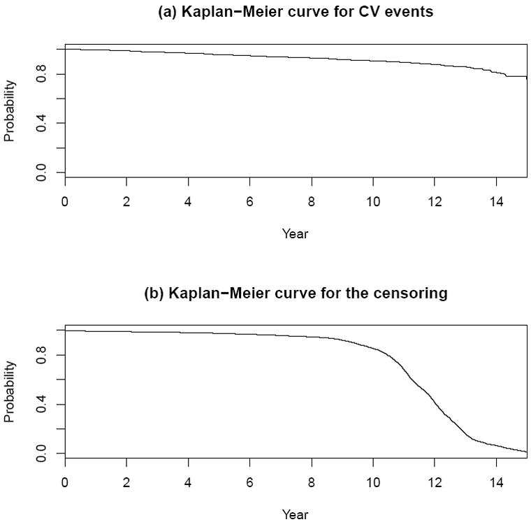
Estimates for survival functions for CV events and censoring variables with Framingham study data.

We fitted the data with a Cox proportional hazards model (2.1). The resulting risk score β̂′Z⁰ is

$$\begin{array}{l}0.54\times (\mathrm{AGE}/10)-0.41\times I(\mathrm{Male})+0.53\times I(\mathrm{SMK}=\mathrm{Yes})\\ +0.40\times (\mathrm{TC}/{10}^2[\mathrm{mg}/\mathrm{dL}])-0.21\times (\mathrm{HDL}/10[\mathrm{mg}/\mathrm{dL}])\\ +0.15\times (\mathrm{SBP}/10[\mathrm{mmHg}])+0.33\times I(\mathrm{TxBP}=\mathrm{Yes}).\end{array}$$

In Table 1, we present point and 0.95 interval estimates of C_τ for various τ. When τ = 8, 10, 12 (years), our results are very similar to those based on the conventional C-index (2.5) procedure with a point estimate of 0.75 and a 0.95 confidence interval of (0.73, 0.77). Note that all the τ-specific conventional C-statistics (2.6) give us similar point and interval estimates. When τ = 14, our estimated standard error for the new C-statistic is markedly larger than that of the conventional method. In this case, study subjects did not have similar follow-up times and it is known that the existing methods in the literature may not work well [13]. Note that all the results reported in Table 1 were based on M = 500 independent realizations of a random sample with n = 3087 from the unit exponential for (A.3).

Table 1.

Point estimates (Est), standard error estimates (SE) and 0.95 confidence intervals (CI) for C_τ with Framingham study data

C-index	New Method			Conventional
τ	Est	SE	CI	Est	SE	CI
8	0.76	0.02	(0.73, 0.79)	0.76	0.01	(0.73, 0.79)
10	0.75	0.01	(0.72, 0.78)	0.75	0.01	(0.73, 0.78)
12	0.75	0.01	(0.72, 0.77)	0.75	0.01	(0.73, 0.78)
14	0.75	0.02	(0.70, 0.80)	0.75	0.01	(0.73, 0.78)
∞	NA	NA	NA	0.75	0.01	(0.73, 0.77)

For τ = 10 (years), we also evaluated the incremental value of HDL cholesterol by comparing the model containing all risk factors described above (Model A) with the model containing risk factors other than HDL cholesterol (Model B). Results of the Cox regression analysis were given in Table 2. The point estimate for $\xi =C_{\tau }^{(A)}-C_{\tau }^{(B)}$ was 0.01, and corresponding 0.95 confidence interval was (-0.00, 0.02). It is interesting to note that although HDL is statistically highly significant with respect to the risk of CV disease in the first 10 years of follow-up, its incremental value evaluated via C-statistics is quite modest.

Table 2.

Estimates of regression parameters for Cox’s models with Framingham study data

	Model A (with HDL)			Model B (without HDL)
	Est.(1)	SE(2)	p(3)	Est.	SE	p
AGE/10 [yrs]	0.54	0.07	0.00	0.53	0.07	0.00
Gender=Male	-0.41	0.12	0.00	-0.63	0.11	0.00
SMK=Yes	0.53	0.13	0.00	0.57	0.12	0.00
TC/102[mg/dL]	0.40	0.15	0.01	0.34	0.15	0.03
SBP/10[mmHg]	0.15	0.03	0.00	0.16	0.03	0.00
IxBP=Yes	0.33	0.12	0.01	0.40	0.12	0.00
HDL/10 [mg/dL]	-0.21	0.04	0.00	-	-	-
	C-index with τ = 10 (0.95 confidence interval)
Conventional	0.75 (0.73, 0.78)			0.74 (0.72, 0.77)
New Method	0.75 (0.72, 0.78)			0.74 (0.71, 0.77)

⁽¹⁾Estimate

⁽²⁾Standard error estimate

⁽³⁾p-value

The second data set for illustration is from a recent cancer study [20]. One primary goal of the study was to evaluate the prognostic value of a new gene signature in predicting the time to death or metastasis for breast cancer patients. An important clinical implications for establishing a risk score system is to identify future patients who may benefit from adjuvant systemic, but potentially toxic, therapies. The details of participants in the study are given in van’t Veer et al. [21] and van de Vijver et al. [22]. The data set for analysis consists of 295 breast cancer patient records from the Netherlands Cancer Institute. Our goal is to evaluate the prediction of patient survival based on the patients’ baseline covariates consisting of the new gene score and other conventional markers including age and estrogen receptor status. The Kaplan-Meier curves for the event time and the censoring time are given in Figure 2. Note that at Year 15, the survival rate is 0.61, the size of the risk set is 19, and there were no deaths beyond this time point. (http://microarray-pubs.stanford.edu/wound_NKI/explore.html).

Figure 2.

Estimates for survival functions for death and censoring variables with breast cancer data.

We fit the data with two working Cox’s proportional hazards models. The covariate vector Z for the first model consists of only age and estrogen receptor (ER: positive or negative). The resulting risk score β̂′Z is

$$-0.47\times (\mathrm{AGE}/10)-1.13\times I(\mathrm{ER}=\mathrm{positive}).$$

In the second model, we included the gene score variable (GS), age and ER. The risk score with the second model is

$$3.28\times (\mathrm{GS})-0.62\times (\mathrm{AGE}/10)-0.70\times I(\mathrm{ER}=\mathrm{positive}).$$

In Table 3, we report the point and interval estimates of C_τ for both models with various τ. Our standard error estimates tend to be larger than those from the conventional C-statistic especially for the case when τ = 15. To examine the performance of the new proposal, we conducted a simulation study. The details are given in the next subsection.

Table 3.

Point estimates (Est), standard error estimates (SE) and 0.95 confidence intervals (CI) for C_τ with breast cancer data

C-index	New Method			Conventional
τ	Est	SE	CI	Est	SE	CI
Without Gene Score Model
6	0.66	0.04	(0.58, 0.74)	0.68	0.04	(0.60, 0.76)
8	0.65	0.04	(0.58, 0.73)	0.68	0.04	(0.60, 0.75)
10	0.65	0.04	(0.57, 0.72)	0.67	0.04	(0.60, 0.74)
15	0.62	0.05	(0.53, 0.71)	0.67	0.04	(0.60, 0.74)
∞*	NA	NA	NA	0.67	0.04	(0.60, 0.74)
With Gene Score Model
6	0.75	0.03	(0.69, 0.82)	0.76	0.03	(0.69, 0.82)
8	0.75	0.03	(0.68, 0.81)	0.75	0.03	(0.69, 0.81)
10	0.74	0.03	(0.68, 0.80)	0.75	0.03	(0.69, 0.81)
15	0.70	0.05	(0.60, 0.79)	0.75	0.03	(0.69, 0.81)
∞*	NA	NA	NA	0.75	0.03	(0.69, 0.81)

^*Note that no event has been seen after t = 15 in the breast cancer data set. All usable pairs in the dataset are already utilized with τ = 15 for calculation of C-statistics. Thus, the estimates for τ = ∞ and those for τ = 15 are identical. With this data set, the censoring probability at t = 15 was 0.89.

3.2. Simulation Study

To examine the performance of the new and conventional methods, we conducted a numerical study under various practical settings. As described in section 2, our proposed inference procedure does not require the fitted model to be correct. Here, we used a working Cox regression model to obtain an estimated risk score, and make inferences about C_τ regardless of the adequacy of the working model. For instance, in one of the simulation settings, we considered two cases with survival time T generated from a Weibull regression model for the first case and from a log-normal regression model for the second case. For both models, we let Z = (AGE, ER, GS)′. We also considered three kinds of censoring: (a) type I censoring without staggered entry; (b) random censoring which is independent of survival time and covariates; and (c) random censoring which is independent of survival time conditional on the covariates. Note that in theory, the existing C-statistics may be valid only for (a). Our procedure is valid for (a) or (b). Setting (c) is explored to examine whether the proposed procedures are sensitive to violation of the independent censoring assumption, as suggested by the reviewers. We chose τ = 10 and 15, and n=100, 150, 200 and 300 for each simulation setting.

Firstly we simulated Z = (AGE, ER, GS)′, utilizing the breast cancer data. In particular, we generated ER status (positive or negative) from its empirical distribution, and then generated the corresponding (AGE, GS) from a multivariate normal distribution, MV N(μ_ER, Σ_ER), where μ_ER and Σ_ER are the empirical mean and variance-covariance matrix of (AGE, GS) conditioning on ER, respectively. For each given value of Z, we generated T from the aforementioned Weibull regression model for case (I) and the log-normal regression model for case (II). We mimicked the breast cancer study to create the true models for our simulation. Specifically, the regression coefficients estimates were obtained by fitting the observed breast cancer data for each model.

With regard to generating censoring time, for censoring type (a), the censoring time D was set as τ + 0.1 for all subjects. For censoring type (b), we fitted the breast cancer data with a one-sample Weibull distribution (with two unknown parameters) to generate D from it. For censoring type (c), we fitted the breast cancer data with a Weibull regression model with the covariate Z = (AGE, ER, GS)′. About 45% of the subjects were censored by Year 10 and 70% by Year 15, which was similar to those from the breast cancer study.

For all simulation configurations, we used a Cox regression model with Z = (AGE, ER, GS)′ as the working model to analyze each simulated data set regardless of whether the true model is the Weibull regression model or the log-normal regression model. Note that this model is correct under the aforementioned Weibull regression and incorrect under the log-normal regression model. For each configuration, we used the monte carlo method to calculate the true values of C_τ for the risk score obtained by fitting the working Cox model. Specifically, we generated one million data points of (T,Z) from each model. The true value for C₁₀ = 0.724 and C₁₅ = 0.718 when the Weibull regression model was true; C₁₀ = 0.727 and C₁₅ = 0.710 when the log-normal regression model was true.

For each setting, we then simulated 1000 independent realizations of {(X_i , Δ_i ,Z_i)′, i = 1, … , n}. We fitted each simulated data set with the working Cox regression model and constructed a 0.95 confidence interval for C_τ given in (2.3). We also constructed the 0.95 confidence interval based on the conventional C-index given by Pencina and D’Agostino [13]. With the 1000 iterations, we obtained empirical coverage probabilities, average lengths of intervals, biases, and root mean square errors (rMSE).

Table 4 shows the results for the case where the working model is correct. When τ = 15 and n = 100 with independent censoring (b), for example, the coverage probabilities of the new and conventional methods are 0.944 and 0.876, respectively. The coverage probability of the new method is 0.946 and still close to the nominal level of 0.95 even under censoring type (c). Table 5 shows the results for the case where the fitted working model is not correct. For τ = 15 and n = 100, the coverage probabilities of the new method are 0.947 and 0.945 under independent and conditionally independent censoring, respectively. On the other hand, those of the conventional method are 0.771 and 0.774, respectively.

Table 4.

Coverage probabilities and average length of 0.95 confidence intervals, bias, and root mean square error (rMSE) for C_τ with τ = 10 and 15, based on 1000 of iterations for a working Cox’s model with (AGE, ER, GS), when the true model is (I) the Weibull regression model with AGE, ER and GS.

			Coverage		Ave. Length		Bias		rMSE
τ	Censoring	N	(1)	(2)	(1)	(2)	(1)	(2)	(1)	(2)
10	(a) Degenerate	100	0.951	0.913	0.214	0.176	0.008	0.008	0.047	0.047
		150	0.945	0.917	0.162	0.145	0.008	0.008	0.038	0.038
		200	0.948	0.934	0.136	0.126	0.005	0.005	0.033	0.033
		300	0.942	0.934	0.108	0.103	0.003	0.003	0.027	0.027
	(b) Independent	100	0.948	0.896	0.241	0.196	0.011	0.015	0.053	0.055
		150	0.952	0.903	0.184	0.163	0.007	0.010	0.043	0.044
		200	0.942	0.914	0.152	0.141	0.009	0.012	0.037	0.039
		300	0.954	0.938	0.122	0.118	0.003	0.007	0.029	0.030
	(c) Cond. Independent	100	0.948	0.892	0.241	0.196	0.011	0.015	0.053	0.055
		150	0.951	0.898	0.184	0.163	0.007	0.010	0.043	0.044
		200	0.946	0.916	0.152	0.142	0.009	0.012	0.037	0.039
		300	0.954	0.937	0.122	0.118	0.003	0.007	0.029	0.030
15	(a) Degenerate	100	0.951	0.912	0.174	0.149	0.006	0.006	0.040	0.040
		150	0.945	0.925	0.134	0.123	0.007	0.007	0.032	0.032
		200	0.956	0.938	0.113	0.107	0.003	0.003	0.027	0.027
		300	0.956	0.944	0.091	0.087	0.002	0.002	0.022	0.022
	(b) Independent	100	0.944	0.876	0.271	0.191	0.011	0.019	0.059	0.055
		150	0.952	0.896	0.207	0.159	0.007	0.015	0.048	0.045
		200	0.932	0.892	0.172	0.138	0.007	0.017	0.042	0.040
		300	0.950	0.926	0.137	0.115	0.003	0.012	0.033	0.031
	(c) Cond. Independent	100	0.946	0.872	0.271	0.192	0.011	0.020	0.059	0.056
		150	0.952	0.894	0.206	0.159	0.007	0.015	0.048	0.045
		200	0.942	0.881	0.173	0.139	0.008	0.017	0.043	0.040
		300	0.951	0.925	0.137	0.115	0.004	0.012	0.033	0.031

⁽¹⁾New Method

⁽²⁾Conventional

Table 5.

Coverage probabilities and average length of 0.95 confidence intervals, bias, and root mean square error (rMSE) for C_τ with τ = 10 and 15, based on 1000 of iterations for a working Cox’s model with (AGE, ER, GS), when the true model is (II) the log-normal regression model with AGE, ER and GS.

			Coverage		Ave. Length		Bias		rMSE
τ	Censoring	N	(1)	(2)	(1)	(2)	(1)	(2)	(1)	(2)
10	a) Degenerate	100	0.947	0.909	0.201	0.165	0.009	0.009	0.045	0.045
		150	0.949	0.923	0.153	0.137	0.007	0.007	0.037	0.037
		200	0.951	0.931	0.128	0.119	0.006	0.006	0.031	0.031
		300	0.953	0.945	0.102	0.097	0.005	0.005	0.025	0.025
	(b) Independent	100	0.947	0.831	0.230	0.179	0.013	0.028	0.050	0.056
		150	0.950	0.858	0.176	0.150	0.007	0.024	0.041	0.046
		200	0.947	0.850	0.146	0.130	0.007	0.023	0.036	0.041
		300	0.926	0.822	0.116	0.106	0.006	0.023	0.030	0.036
	(c) Cond. Independent	100	0.945	0.837	0.230	0.179	0.013	0.028	0.050	0.056
		150	0.942	0.859	0.175	0.150	0.008	0.024	0.042	0.046
		200	0.950	0.853	0.146	0.130	0.007	0.023	0.036	0.041
		300	0.928	0.813	0.116	0.106	0.006	0.023	0.030	0.036
15	a) Degenerate	100	0.953	0.921	0.170	0.144	0.006	0.006	0.039	0.039
		150	0.960	0.935	0.131	0.119	0.004	0.004	0.031	0.031
		200	0.960	0.945	0.111	0.103	0.003	0.003	0.026	0.026
		300	0.949	0.944	0.088	0.085	0.002	0.002	0.022	0.022
	(b) Independent	100	0.947	0.771	0.263	0.175	0.011	0.043	0.060	0.063
		150	0.949	0.789	0.201	0.146	0.008	0.039	0.046	0.054
		200	0.943	0.751	0.168	0.127	0.007	0.038	0.041	0.050
		300	0.944	0.683	0.135	0.104	0.004	0.038	0.033	0.047
	(c) Cond. Independent	100	0.945	0.774	0.264	0.175	0.011	0.043	0.060	0.063
		150	0.944	0.788	0.200	0.146	0.009	0.039	0.046	0.055
		200	0.937	0.743	0.168	0.127	0.007	0.038	0.041	0.050
		300	0.939	0.682	0.135	0.104	0.005	0.038	0.033	0.047

⁽¹⁾New Method

⁽²⁾Conventional

In general, we find that the new interval estimation procedure performs well with relatively small sample size, regardless of the adequacy of the fitted model. Furthermore, the procedure is not sensitive to violation of the covariate independent censoring assumption with empirical coverage levels practically identical to their nominal counterparts under various situations. The conventional method proposed by Pencina and D’Agostino [13] performs well when the censoring distribution is a degenerate distribution (Type I censoring without staggered entry).

4. REMARKS

In this article, we show that the overall performance of a parametric or semi-parametric model in predicting the subject-level survival over an interval (0, τ) can be evaluated via a simple, unbiased estimation procedure for C_τ. Based on our numerical study, we find that the new estimation procedure is robust with respect to the choice of τ. However, if the pre-specified τ is “too” large such that very few events were observed or very few study subjects were followed beyond this time point, the standard error estimate for Ĉ_τ can be quite large, reflecting a high degree of uncertainty of our inferences about C_τ. For this case, one should cautiously utilize the fitted model for prediction over this large time interval.

There are various C-statistics proposed in the literature. With the same technique utilized in this article, one may modify these statistics accordingly so that they estimate concordance measures which are free of the study-specific censoring distribution. The computer code for implementing the new inference procedure can be downloaded from (http://bcb.dfci.harvard.edu/~huno).

For the new proposal, we assume that the censoring distribution is independent of the covariates. This assumption is not unreasonable in a well-executed clinical study, especially when there are no competing risks for observing the endpoint (for example, death or a composite clinical endpoint) and the event times are possibly censored mainly due to administrative censoring. When the covariate vector can be discretized, our new procedure can be modified easily using stratified Kaplan-Meier estimates for the censoring. When some of the covariates are continuous, one needs to assume a model for censoring distribution and use the resulting estimated distribution of the censoring to construct a new C-statistic. In theory, the validity of the resulting estimators depends on the adequacy of the model. On the other hand, based on the results from our simulation study, it appears that our proposal is quite robust even when the censoring is dependent on the covariates.

In this article, we showed an inference procedure not only for C_τ but also for the difference between two C_τ ’s for comparing two competing prediction models. Although C-statistics are commonly used for quantifying the predictability of working models, they are not sensitive for capturing overall added values from a new marker on top of conventional predictors [11, 13]. Alternatively, one might use measures such as explained variation for survival data to compare two models [7]. If the model is correct, the likelihood based measures may be more sensitive in detecting differences in prediction ability, compared to rank-based measures such as C-indexes. Recently, alternative statistical estimation procedures were proposed for comparing prediction models [23, 24], which may be utilized to quantify incremental values. Further research is needed for developing intuitively interpretable and sensitive methods for comparing prediction models.

APPENDIX A: LARGE SAMPLE PROPERTIES OF Ĉ_τ

Throughout, we assume that the non-separable condition for (T,Z) given in section 2 holds, and thus β₀ is the unique solution to the limit of the following partial likelihood score equation,

$$U(\beta )=n^{-1}\sum _{i=1}^n{U}_i(\beta )=n^{-1}\sum _{i=1}^n{\mathit{\int }}_0^{\tau }\left\{Z_i-\frac{{\sum }_j{Y}_j(t)\exp ({\beta }^{\prime }{Z}_j)Z_j}{{\sum }_j{Y}_j(t)\exp ({\beta }^{\prime }{Z}_j)}\right\}{\mathit{dN}}_i(t)=0,$$

where N_i(t) = I(X_i ≤ t, Δ_i = 1), Y_i(t) = I(X_i ≥ t). We assume that β₀ lies in a compact parameter space and the joint density of (T, Z) is continuous and bounded. To show the consistency of Ĉ_τ , we first note that

$$n^{1/2}\left(\widehat{\beta }-{\beta }_0\right)=n^{-1/2}\sum _{i=1}^{n}A\left({\beta }_0\right)U_i\left({\beta }_0\right)+O_p\left(n^{-1}\right)$$ (A.1)

where A(β) = − {∂E(U(β))/∂β}⁻¹ [25].

Now, for a fixed β, let

$$C_{\tau }(\beta )=\mathrm{pr}({\beta }^{\prime }{Z}_1^0>{\beta }^{\prime }{Z}_2^0\mid T_1^0<T_2^0,T_1^0<\tau ).$$

It follows from the uniform consistency of Ĝ(·), the convergence of β̂ to β₀, and a uniform law of large numbers for U-processes [26], that Ĉ_τ converges to C_τ(β₀) in probability as n → ∞. On the other hand, it follows from the asymptotic expansion of β̂ given in (A.1) that C_τ(β₀) − C_τ = O(n⁻¹). Thus, Ĉ_τ − C_τ → 0 in probability.

To approximate the distribution of

$$W=n^{\frac{1}{2}}\left\{{\widehat{C}}_{\tau }(\widehat{\beta })-C_{\tau }\right\},$$

we first obtain asymptotic expansions for W(β) = n^1/2{Ĉ_τ(β) − C_τ(β)}, where Ĉ_τ(β) is obtained by replacing β̂ in Ĉ_τ of (2.4) with β. To this end, we write W(β) = W_a(β) + W_b(β), where

$$W_a(\beta )=n^{1/2}\frac{{\sum }_{i=1}^n{\sum }_{j=1}^n{I}_{\mathit{ij}}(\tau )G{(X_i)}^{-2}\left\{I({\beta }^{\prime }{Z}_i>{\beta }^{\prime }{Z}_j)-C_{\tau }(\beta )\right\}}{{\sum }_{i=1}^n{\sum }_{j=1}^n\widehat{G}{(X_i)}^{-2}{I}_{\mathit{ij}}(\tau )},$$

$$W_b(\beta )=n^{1/2}\frac{{\sum }_{i=1}^n{\sum }_{j=1}^n\left\{\widehat{G}{(X_i)}^{-2}-G{(X_i)}^{-2}\right\}{I}_{\mathit{ij}}(\tau )\left\{I({\beta }^{\prime }{Z}_i>{\beta }^{\prime }{Z}_j)-C_{\tau }(\beta )\right\}}{{\sum }_{i=1}^n{\sum }_{j=1}^n\widehat{G}{(X_i)}^{-2}{I}_{\mathit{ij}}(\tau )}$$

and I_ij(τ) = I(X_i < X_j, X_i < τ)Δ_i. Now, it follows from the standard asymptotic theory for the Kaplan Meier estimator [27],

$${\widehat{W}}_G(t)=\frac{n^{1/2}\left\{G(t)-\widehat{G}(t)\right\}}{G(t)}\approx n^{-1/2}\sum _{i=1}^n{\psi }_i(t)$$

and Ŵ_G(t) converges weakly to a zero-mean Gaussian process indexed by t for t ≤ τ, where ${\psi }_i(t)={\mathit{\int }}_0^t{\mathit{dM}}_i(u)/{\pi }_X(u),{\pi }_X(t)=\mathrm{pr}(X_i\ge t)$ and $M_i(t)=I(X_i\le t,{\mathrm{\Delta }}_i=0)-{\mathit{\int }}_0^{t}I(X_i\ge u)d{\mathrm{\Lambda }}_D(u)$, Λ_D(·) is the cumulative hazard function for the common censoring variable. Also, it follows from the uniform consistency of Ĝ(·) and a functional central limit theorem for U-processes [28] that

$$W_a(\beta )=n^{-3/2}p{(\tau )}^{-1}\sum _{i=1}^n\sum _{j=1}^{n}G{(X_i)}^{-2}{I}_{\mathit{ij}}(\tau )\left\{I({\beta }^{\prime }{Z}_i>{\beta }^{\prime }{Z}_j)-C_{\tau }(\beta )\right\}+o_p(1),$$

where p(τ) = P(T₁ < T₂, T₁ < τ). Furthermore,

$$W_b(\beta )={\mathit{\int }}_0^{\tau }{n}^{1/2}\left\{\frac{G{(t)}^2}{\widehat{G}{(t)}^2}-1\right\}d\widehat{\gamma }(t,\beta )$$

where

$$\widehat{\gamma }(t,\beta )=\frac{{\sum }_{i=1}^n{\sum }_{j=1}^{n}G{(X_i)}^{-2}I(X_i\le t)I_{\mathit{ij}}(\tau )\{I({\beta }^{\prime }{Z}_i>{\beta }^{\prime }{Z}_j)-C_{\tau }(\beta )\}}{{\sum }_{i=1}^n{\sum }_{j=1}^n\widehat{G}{(X_i)}^{-2}{I}_{\mathit{ij}}(\tau )}.$$

By a uniform law of large numbers for U-processes [26] and the uniform consistency of Ĝ(·), we have

$$\underset{t\in [0,\tau ],\beta }{\sup }\mid \widehat{\gamma }(t,\beta )-\gamma (t,\beta )\mid \to 0,\mathrm{in\; probability}$$

where

$$\gamma \left(t,\beta \right)=\frac{p\left(t\right)\{\mathrm{pr}\left({\beta }^{\prime }{Z}_i>{\beta }^{\prime }{Z}_j\mid T_i<T_j,T_i<t\right)-C_{\tau }\left(\beta \right)\}}{p\left(\tau \right)}.$$

This, coupled with the weak convergence of Ŵ_G(t), implies that

$$W_b(\beta )=2\mathit{\int }{\widehat{W}}_G(t)d\gamma (t,\beta )+o_p(1)=n^{-1/2}\sum _{i=1}^{n}2\mathit{\int }{\psi }_i(t)d\gamma (t,\beta ).$$

Therefore,

$$W\left(\beta \right)={\left(\begin{array}{c}n\\ 2\end{array}\right)}^{-1}\sum _{i<j}\{{\nu }_{\mathit{ij}}(\beta )+{\varphi }_{\mathit{ij}}(\beta )\}+o_p(1),$$

where ν_ij(β) = (V_ij(β) + V_ij(β))/2,

$$V_{\mathit{ij}}\left(\beta \right)=p{\left(\tau \right)}^{-1}G{\left(X_i\right)}^{-2}{I}_{\mathit{ij}}\left(\tau \right)\{I\left({\beta }^{\prime }{Z}_i>{\beta }^{\prime }{Z}_j\right)-C_{\tau }\left(\beta \right)\},$$

and φ_ij(β) = ∫ {ψ_i(t) + ψ_j(t)} dγ(t, β). It then follows from a functional central limit theorem for U-processes that W(β) converges weakly to a zero-mean Gaussian process. This, together with the continuity of C_τ(β) and the asymptotic expansion of n^1/2(β̂ − β₀), implies that

$$W=W\left({\beta }_0\right)+{\dot{C}}_{\tau }\left({\beta }_0\right)n^{1/2}\left(\widehat{\beta }-{\beta }_0\right)+o_p\left(1\right)={\left(\begin{array}{c}n\\ 2\end{array}\right)}^{-1}\sum _{i<j}{W}_{\mathit{ij}}+o_p\left(1\right)$$ (A.2)

where Ċ_τ(β) = ∂C_τ (β)/∂β and

$$W_{\mathit{ij}}={\nu }_{\mathit{ij}}\left({\beta }_0\right)+{\varphi }_{\mathit{ij}}\left({\beta }_0\right)+{\dot{C}}_{\tau }\left({\beta }_0\right)A\left({\beta }_0\right)\{U_i\left({\beta }_0\right)+U_j\left({\beta }_0\right)\}/2.$$

This, together with the standard asymptotic theory of U-statistics, W is asymptotically normal with mean 0 and variance E(W₁₂W₁₃).

To estimate the variance of W, we utilize a perturbation-resampling method which has been successfully used for handling numerous inference problems in survival analysis [29, 30]. To be specific, let {Ξ_i, i = 1, … n} be a set of n iid random variables from a known distribution with mean 1 and variance 1. For a large n, we can approximate W with the conditional distribution (conditional on the data) of

$$\stackrel{\sim }{W}={\left(\begin{array}{c}n\\ 2\end{array}\right)}^{-1}\sum _{i<j}{\widehat{\nu }}_{\mathit{ij}}\left(\widehat{\beta }\right){\mathrm{\Xi }}_i{\mathrm{\Xi }}_j+n^{1/2}\{\widehat{K}\left(G^{\ast }\right)-\widehat{K}\left(\widehat{G}\right)\}+n^{1/2}\{{\widehat{C}}_{\tau }\left({\beta }^{\ast }\right)-{\widehat{C}}_{\tau }\left(\widehat{\beta }\right)\},$$ (A.3)

where

$$\widehat{K}\left(G\right)=\widehat{p}{\left(\tau \right)}^{-1}{\left(\begin{array}{c}n\\ 2\end{array}\right)}^{-1}\sum _{i<j}G{\left(X_i\right)}^{-2}{I}_{\mathit{ij}}\left(\tau \right)\{I\left({\widehat{\beta }}^{\prime }{Z}_i>{\widehat{\beta }}^{\prime }{Z}_j\right)-{\widehat{C}}_{\tau }\left(\widehat{\beta }\right)\},$$

$\widehat{p}(\tau )=n^{-2}{\sum }_{i=1}^n{\sum }_{j=1}^n\widehat{G}{(X_i)}^{-2}{I}_{\mathit{ij}}(\tau )$, and G* (·) and β* are the corresponding perturbed versions of Ĝ(·) and β̂. Specifically, G* (t) is generated by

$$G^{\ast }(t)=\widehat{G}(t)-\widehat{G}(t){\left(\begin{array}{c}n\\ 2\end{array}\right)}^{-1}\sum _{i<j}{\mathit{\int }}_0^t{\widehat{\pi }}_X^{-1}(u)\left\{d{\widehat{M}}_i(u)+d{\widehat{M}}_j(u)\right\}{\mathrm{\Xi }}_i{\mathrm{\Xi }}_j/2$$

where ${\widehat{\pi }}_X(u)=n^{-1}{\sum }_{i=1}^{n}I(X_i\ge u)$, ${\widehat{M}}_i(t)=I(X_i\le t,{\mathrm{\Delta }}_i=0)-{\mathit{\int }}_0^{t}I(X_i\ge u)d{\widehat{\Lambda }}_D(u)$ and Λ̂_D(·) is a consistent estimator of the cumulative hazard function for the censoring variable. We generate β* as

$${\beta }^{\ast }=\widehat{\beta }+{\left(\begin{array}{c}n\\ 2\end{array}\right)}^{-1}\sum _{i<j}\left[\widehat{A}(\widehat{\beta })\{U_i(\widehat{\beta })+U_j(\widehat{\beta })\}/2\right]{\mathrm{\Xi }}_i{\mathrm{\Xi }}_j.$$

Note that only the random quantity in W̃ is {Ξ_i, i = 1,…,n}. The unknown quantities are replaced with their empirical counterparts. The distribution of W̃ (and therefore the distribution of W) can be approximated by generating a large number of realized random samples from {Ξ_i, i = 1,…n}.

APPENDIX B: LARGE SAMPLE APPROXIMATION TO W_ξ

From (A.2), W_ξ is denoted by ${\left(\begin{array}{c}n\\ 2\end{array}\right)}^{-1}{\sum }_{i<j}(W_{\mathit{ij}}^{(A)}-W_{\mathit{ij}}^{(B)})+o_p(1)$, where $W_{\mathit{ij}}^{(A)}$ and $W_{\mathit{ij}}^{(B)}$ correspond to W_ij in (A.2) for Model A and Model B, respectively. Thus, W_ξ is asymptotically normal with mean 0 and variance $E\{(W_{12}^{(A)}-W_{12}^{(B)})(W_{13}^{(A)}-W_{13}^{(B)})\}$. To estimate the variance of W_ξ, let W̃^(A) and W̃^(B) be the approximation to $W^{(A)}=n^{\frac{1}{2}}({\widehat{C}}_{\tau }^{(A)}-C_{\tau }^{(A)})$ and $W^{(B)}=n^{\frac{1}{2}}({\widehat{C}}_{\tau }^{(B)}-C_{\tau }^{(B)})$ by the perturbation described above, respectively. Let ${\stackrel{\sim }{W}}_k^{(A)}$ and ${\stackrel{\sim }{W}}_k^{(B)}$ be a pair of realizations obtained with the k^th set of random variables {Ξ_i, i = 1,…n}. Then, the distribution of W_ξ can be numerically approximated by a large number of M realizations of ${\stackrel{\sim }{W}}_k^{(A)}-{\stackrel{\sim }{W}}_k^{(B)},k=1,\dots ,M$.

References

- 1.Anderson KM, Odell PM, Wilson PW, Kannel WB. Cardiovascular risk profiles. American Heart Journal. 1991;121:293–8. doi: 10.1016/0002-8703(91)90861-b. [DOI] [PubMed] [Google Scholar]
- 2.D’Agostino RB, Vasan RS, Pencina MJ, Wolf PA, Cobain MR, Massaro JM, Kannel WB. General cardiovascular risk profile for use in primary care: The Framingham Heart Study. Circulation. 2008;117(6):743–53. doi: 10.1161/CIRCULATIONAHA.107.699579. [DOI] [PubMed] [Google Scholar]
- 3.Shariat SF, Karakiewicz PI, Roehrborn CG, Kattan MW. An updated catalog of prostate cancer predictive tools. Cancer. 2008;113(11):3075–99. doi: 10.1002/cncr.23908. [DOI] [PubMed] [Google Scholar]
- 4.Parikh NI, Pencina MJ, Wang TJ, Benjamin EJ, Lanier KJ, Levy D, D’Agostino RB, Sr, Kannel WB, Vasan RS. A risk score for predicting near-term incidence of hypertension: the Framingham Heart Study. Annals of Internal Medicine. 2008;148(2):102–10. doi: 10.7326/0003-4819-148-2-200801150-00005. [DOI] [PubMed] [Google Scholar]
- 5.Bamber D. The area above the ordinal dominance graph and the area below the receiver operating characteristic graph. Journal of Mathematical Psychology. 1975;12:387–415. [Google Scholar]
- 6.Hanley JA, McNeil BJ. The meaning and use of the area under a receiver operating characteristic (ROC) curve. Radiology. 1982;143:29–36. doi: 10.1148/radiology.143.1.7063747. [DOI] [PubMed] [Google Scholar]
- 7.Korn EL, Simon R. Measures of explained variation for survival data. Statistics in Medicine. 1990;9:487–503. doi: 10.1002/sim.4780090503. [DOI] [PubMed] [Google Scholar]
- 8.Hielscher T, Zucknick M, Werft W, Benner A. On the prognostic value of survival models with application to gene expression signatures. Statistics in Medicine. 2010;29:818–829. doi: 10.1002/sim.3768. [DOI] [PubMed] [Google Scholar]
- 9.Harrell FE, Califf RM, Pryor DB, Lee KL, Rosati RA. Evaluating the yield of medical tests. Journal of the American Medical Association. 1982;247:2543–46. [PubMed] [Google Scholar]
- 10.Harrell FE, Lee KL, Califf RM, Pryor DB, Lee KL, Rosati RA. Regression modeling strategies for improved prognostic prediction. Statistics in Medicine. 1984;3:143–52. doi: 10.1002/sim.4780090503. [DOI] [PubMed] [Google Scholar]
- 11.Harrell FE, Lee KL, Mark DB. Tutorial in Biostatistics: Multivariable prognostic models: issues in developing models, evaluating assumptions and adequacy, and measuring and reducing errors. Statistics in Medicine. 1996;15:361–87. doi: 10.1002/(SICI)1097-0258(19960229)15:4¡361∷AID-SIM168¿3.0.CO;2-4. [DOI] [PubMed] [Google Scholar]
- 12.Brown BW, Hollander M, Korwar RM. Nonparametric tests of independence for censored data, with applications to heart transplant studies. In: Proschan F, Serfling RJ, editors. Reliability and Biometry. SIAM; Philadelphia: 1974. [Google Scholar]
- 13.Pencina MJ, D’Agostino RB. Overall C as a measure of discrimination in survival analysis: model specific population value and confidence interval estimation. Statistics in Medicine. 2004;23:2109–23. doi: 10.1002/sim.1802. [DOI] [PubMed] [Google Scholar]
- 14.Heagerty PJ, Zheng Y. Survival model predictive accuracy and ROC curves. Biometrics. 2005;61:92–105. doi: 10.1111/j.0006-341X.2005.030814.x. [DOI] [PubMed] [Google Scholar]
- 15.Chambless LE, Diao G. Estimation of time-dependent area under the ROC curve for long-term risk prediction. Statistics in Medicine. 2006;25:3474–3486. doi: 10.1002/sim.2299. [DOI] [PubMed] [Google Scholar]
- 16.Cai T, Pepe MS, Zheng Y, Lumley T, Jenny NS. The sensitivity and specificity of markers for event times. Biostatistics. 2006;72:182–97. doi: 10.1093/biostatistics/kxi047. [DOI] [PubMed] [Google Scholar]
- 17.Gönen M, Heller G. Concordance probability and discriminatory power in proportional hazards regression. Biometrika. 2005;92:965–970. doi: 10.1093/biomet/92.4.965. [DOI] [Google Scholar]
- 18.Cox DR. Regression models and life tables (with Discussion) Journal of the Royal Statistical Society, Ser B. 1972;34:187–220. [Google Scholar]
- 19.Cheng SC, Wei LJ, Ying Z. Analysis of transformation models with censored data. Biometrika. 1995;82:835–845. doi: 10.1093/biomet/82.4.835. [DOI] [Google Scholar]
- 20.Chang HY, Nuyten DSA, Sneddon JB, Hastie T, Tibshirani R, Sørlieb T, Dai H, He YD, van’t Veer LJ, Bartelinke H, van de Rijnj M, Brownb PO, van de Vijver MJ. Robustness, scalability, and integration of a wound-response gene expression signature in predicting breast cancer survival. PNAS. 2005;102:3738–43. doi: 10.1073/pnas.0409462102. [DOI] [PMC free article] [PubMed] [Google Scholar]
- 21.van’t Veer LJ, Dai H, van de Vijver MJ, He YD, Hart AA, Mao M, Peterse HL, van der Kooy K, Marton MJ, Witteveen AT. Gene expression profiling predicts clinical outcome of breast cancer. Nature. 2002;415:530–6. doi: 10.1038/415530a. [DOI] [PubMed] [Google Scholar]
- 22.van de Vijver MJ, He YD, van’t Veer LJ, Dai H, Hart AAM, Voskuil DW, Schreiber GJ, Peterse JL, Roberts C, Marton MJ, Parrish M, Atsma D, Witteveen A, Glas A, Delahaye L, van der Velde T, Bartelink H, Rodenhuis S, Rutgers ET, Friend SH, Bernards R. A gene-expression signature as a predictor of survival in breast cancer. The New England Journal of Medicine. 2002;347:1999–2009. doi: 10.1056/NEJMoa021967. [DOI] [PubMed] [Google Scholar]
- 23.Pencina MJ, D’Agostino RB, Sr, D’Agostino RB, Jr, Vasan RS. Evaluating the added predictive ability of a new marker: From area under the ROC curve to reclassification and beyond. Statistics in Medicine. 2008;27:157–72. doi: 10.1002/sim.2929. [DOI] [PubMed] [Google Scholar]
- 24.Cai T, Tian L, Lloyd-Jones DM, Wei LJ. Evaluating subject-level incremental values of new markers for risk classification rule. Harvard University Biostatistics Working Paper Series. 2008 doi: 10.1007/s10985-013-9272-6. Working Paper 91. http://www.bepress.com/harvardbiostat/paper91. [DOI] [PMC free article] [PubMed]
- 25.Hjort N. On inference in parametric survival data models. International Statistical Review. 1992;60:355–87. [Google Scholar]
- 26.Nolan D, Pollard D. U-processes: Rates of convergence. The Annals of Statistics. 1987;15:780–99. [Google Scholar]
- 27.Kalbfleisch JD, Prentice RL. The Statistical Analysis of Failure Time Data. 2. Wiley; New York: 2002. [Google Scholar]
- 28.Nolan D, Pollard D. Functional limit theorems for U-processes. The Annals of Statistics. 1988;16:1291–98. [Google Scholar]
- 29.Lin DY, Wei LJ, Ying Z. Checking the Cox model with cumulative sums of martingale-based residuals. Biometrika. 1993;80:557–72. doi: 10.1093/biomet/80.3.557. [DOI] [Google Scholar]
- 30.Lin DY, Fleming TR, Wei LJ. Confidence bands for survival curves under the proportional hazards model. Biometrika. 1994;81:73–81. doi: 10.1093/biomet/81.1.73. [DOI] [Google Scholar]