

Abstract
Delay discounting describes the decline in the value of a reinforcer as the delay to that reinforcer increases. A review of the available studies revealed that steep delay discounting is positively correlated with problem or pathological gambling. One hypothesis regarding this correlation derives from the discounting equation proposed by Mazur (1989). According to the equation, steeper discounting renders the difference between fixed-delayed rewards and gambling-like variable-delayed rewards larger; with the latter being more valuable. The present study was designed to test this prediction by first assessing rats’ impulsive choices across four delays to a larger-later reinforcer. A second condition quantified strength of preference for mixed- over fixed-delays, with the duration of the latter adjusted between sessions to achieve indifference. Strength of preference for the mixed-delay alternative is given by the fixed delay at indifference (lower fixed-delay values reflect stronger preferences). Percent impulsive choice was not correlated with the value of the fixed delay at indifference and, therefore, the prediction of the hyperbolic model of gambling was not supported. A follow-up assessment revealed a significant decrease in impulsive choice after the second condition. This shift in impulsive choice could underlie the failure to observe the predicted correlation between impulsive choice and degree of preference for mixed- over fixed delays.
Keywords: Delay discounting, impulsivity, delay, gambling, rat
Delay discounting describes the devaluation of an event as the delay to that event increases. Steep delay discounting describes a specific form of impulsive choice: preference for a smaller-sooner over a larger-later reward and the opposite preference involving aversive events. A number of studies using human participants have revealed a correlation between the degree to which the value of delayed monetary events is discounted and substance use disorders (see review by Yi et al., 2010). What underlies this correlation is not well understood. Evidence suggesting that steep delay discounting is predictive of drug taking comes, for example, from studies demonstrating that steep discounting of delayed food rewards precedes and predicts drug self-administration in rodents (see review by Carroll et al., 2010). The opposite, though not incompatible, relation would be supported if acute or chronic drug administration increases impulsivity and/or renders delay discounting curves steeper. At present, the effects of acute drugs of abuse on delay discounting are mixed; with ethanol and nicotine producing the most consistent increases in impulsive choice when assessed with nonhuman animals (see review by de Wit & Mitchell, 2010). Less work has explored chronic drug administration, but some evidence suggests chronic nicotine and cocaine increase impulsive choice after dosing or self-administration concludes (see review by Setlow et al., 2009).
A less extensive literature suggests a similar relation exists between steep delay discounting and gambling disorders in humans (see Table 1). Most studies of this relation have recruited participants based on their answers to the South Oaks Gambling Screen (SOGS; Lesieur & Blume, 1987). Scores of 5 and above are widely regarded as indicative of pathological gambling (for a discussion of the possible leniency of this criterion see Stinchfield, 2002). In the first of these studies, Petry and Casarella (1999) reported that substance abusers with SOGS scores of 5 and higher more steeply discounted delayed monetary rewards than did substance abusers who rarely gambled, and more than controls who had no prior history of substance use or gambling disorders. Dixon et al. (2003) reported a similar outcome when they compared delay discounting between gamblers in an off-track betting facility and controls in a non-gambling setting. A follow-up study revealed less steep delay discounting when gamblers completed the task in a non-gambling context (Dixon et al., 2006); nonetheless, the difference between gamblers and controls remained significant when context was constant across groups (see reanalysis by Petry & Madden, 2010).
Table 1.
Characteristics of, and findings reported in studies evaluating the relation between delay discounting and gambling.
| Authors | Mean SOGS Scores (N) |
Discounting Task | Delayed Outcomes | Results | ||
|---|---|---|---|---|---|---|
| Gamblers | Controls | Other | ||||
| Petry & Casarella (1999) | 9.5 (29)‡ | NR (18) | <1 (34)† | Rachlin et al. (1991) | $100 & $1,000 (hypothetical) | Problem gambling substance abusers discounted more steeply than other groups |
| Petry (2001) | 12.0 (39)* | 0.7 (26) | 13.8 (21)*‡ | Rachlin et al. (1991) | $1,000 (hypothetical) | Significant linear contrast with steepest discounting among substance abusing pathological gamblers. |
| Dixon et al. (2003) | 5.8 (20)§ | 0.7 (20) | Rachlin et al. (1991) | $1,000 (hypothetical) | Steeper discounting among gamblers | |
| Holt et al. (2003) | 6.5 (19) | 0.3 (19) | 6-choice adj-amount | $1,000 & $50,000 (hypothetical) | No significant effect of group on delay discounting. Significant difference in probability discounting. | |
| Dixon et al. (2006) | 6.6 (20)§ | Rachlin et al. (1991) | $1,000 (hypothetical) | Within-Ss design: Steeper discounting when gamblers completed task in gambling setting | ||
| MacKillop et al. (2006) | 7.7 (24) | 0.0 (40) | 1.8 (41) | Rachlin et al. (1991) | $1,000 (hypothetical) | Gamblers discounted more steeply than controls. No other differences were significant. |
| Ledgerwood et al. (2009) | 7.1Ω | 0.2Ω (41) | 7.4Ω (31)‡ | Rachlin et al. (1991) | $1,000 (hypothetical) | Both groups of gamblers discounted more steeply than controls, but no difference between gamblers with and without history of substance use disorder |
| Madden et al. (2009) | 13.3 (19)* | 0.8(19) | Kirby & Maraković (1995) | ≤ $85 (hypothetical) | Steeper discounting in pathological gamblers approached significance when differences in education and ethnicity were included as covariates | |
NR: Not reported
DSM-IV or NODS diagnosis of pathological gambling
Substance abusing gamblers
Substance abusers who rarely or never gambled
Delay discounting assessed in an off-track betting facility
Prior year NODS score (SOGS scores not reported). A NODS score of ≥ 5 is indicative of pathological gambling according to DSM IV criteria.
Two studies have examined the relation between gambling and delay discounting among college-student gamblers. Holt et al. (2003) reported no difference in delay discounting between gambling and non-gambling students. Based on the SOGS scores shown in Table 1, this is a somewhat surprising finding because mean SOGS scores were in the range reported for gamblers in the Dixon et al. (2003, 2006) studies. Using similar methods with larger sample sizes, and assigning participants to groups using a slightly more stringent SOGS criterion, MacKillop et al. (2006) reported that student gamblers more steeply discounted delayed monetary outcomes than did non-pathological gambling controls.
A final category of these studies are those comparing delay discounting between controls and gamblers meeting either the DSM IV (American Psychiatric Association, 1994) criteria for pathological gambling or the National Opinion Research Center DSM Screen for Gambling Problems (NODS; Gerstein et al., 1999). Petry (2001) reported the steepest delay discounting among dual-diagnosed substance abusing pathological gamblers, less steep discounting in pathological gamblers with no history of substance-use disorder, and more-shallow discounting among controls. Ledgerwood et al. (2009) systematically replicated the difference in discounting between pathological gamblers and controls, but not between gamblers with and without a diagnosed substance-use disorder. Finally, Madden et al. (2009) examined delay discounting among pathological gamblers and matched controls using the brief paper and pencil measure developed by Kirby and Maraković, (1995). The between-group difference in estimated discounting rate approached, but did not achieve statistical significance. Thus, with few exceptions (Holt et al., 2003; Madden et al., 2009) there is a positive relation between steep delay discounting and problem gambling. Indeed, Alessi and Petry’s (2003) reanalysis of data collected by Petry and Casarella (1999) and Petry (2001) revealed that the best predictor of degree of delay discounting was severity of the gambling disorder (as measured by the SOGS).
A shortcoming of this literature is that delay discounting is assessed after participants have engaged in problem gambling. Thus, we know these tendencies are positively correlated, but we do not know if a) steep delay discounting precedes and predicts a stronger preference for gambling, b) prolonged gambling activity affects the discounting of delayed outcomes, or c) a third variable accounts for the correlation.
Available theories regarding this relation speculate on why steep delay discounting may affect subsequent decisions to gamble. A general addiction-related theory was suggested by Odum et al. (2000). They suggested that steeply discounting the delayed losses associated with any addiction (e.g., eventual loss of vocation, spouse, friends) would render these prospective losses inert in the decision to continue the behavior.
In a more gambling-specific account known as “string theory,” Rachlin (1990) suggested that the functional unit in the gambling milieu is the temporally extended string of wagers concluding in a win. The string may be as short as a single wager ending in a win and has no upper bound on the number of losses that may precede the win that terminates the string. According to string theory, the value of the gambling prospect is the sum of the discounted values of previously experienced strings; we have represented this using the equation proposed by Mazur (1989):
| (1) |
In Equation 1, V is the value of the prospective gambling string and Pi is the probability of experiencing each different delay, Di (string length), to a gambling win. The net value of the string, N, is the sum of the win and the losses (if any) in the string (e.g., assuming three $1 and one $2 wagers are lost before a $10 win, the net value of the string is $5). Finally, k is the discounting parameter which increases as the delay discounting curve descends more steeply.
String theory’s account of the relation between steep delay discounting and propensity to gamble is as follows. Short strings have an objective net gain (e.g., win $10 on the first bet; N = $10), while long strings produce a net loss (e.g., 23 $1 losses concluding with a $10 win; N = −$13). The decision making of a steep delay discounter is largely unaffected by losses because they occur at the end of long strings; thus this net loss is substantially discounted and when summed with undiscounted net gains following short strings yields a positively valued gambling prospect (V). By contrast, shallow discounting means that net losses at the end of long strings retain much of their negative value; thereby rendering negative the overall value of the gambling prospect. Thus, string theory predicts the empirically observed relation between steep delay discounting and problem gambling.
A third accounting of the relation between steep delay discounting and problem gambling is structurally similar to string theory, but its focus is not on discounting net gains and losses but on the quantitative implications of the shape of the discounting curve for the relative valuation of gambling and non-gambling rewards (Madden et al., 2005). A critical component of this account is that the delay to a gambling win is variable and, therefore, unpredictable; whereas the delay to a non-gambling reward is predictable. The value of the unpredictably delayed gambling prospect (Vu) is determined by the hyperbolic delay discounting equation proposed by Mazur (1989):
| (2) |
where the parameters are as in Equation 1 but N is replaced by the amount (A) of the gambling win1. The value of the non-gambling prospect is determined by the simpler version of Mazur’s (1987) hyperbolic discounting equation, in which the delay is the same every time.
Consistent with the findings reviewed by Kacelnik and Bateson (1996), and the results of a recent human-subject experiment conducted by Locey et al. (2009), Equation 2 predicts that gambling-like variable delays to a reinforcer will be preferred over fixed delays regardless of the value of k. The top panel of Figure 1 illustrates a simplified version of this prediction. In this graph, k = 1.0; a value commonly observed with pigeons. The open data point represents a fixed delay (FD) to reinforcement of 10 s. At k=1.0, the value of this reinforcer is discounted by approximately 95%. The solid data points illustrate the discounted values of two reinforcers; one delivered 0 s after a response and the other after a 20 s delay; a mixed-delay (MD) arrangement. Assuming equal probabilities, the probability-weighted duration of the MD is the same as the FD (10 s), but the overall discounted value of the MD prospect, given by the horizontal dashed line, is considerably higher (52% vs. approximately 5%).
Figure 1.
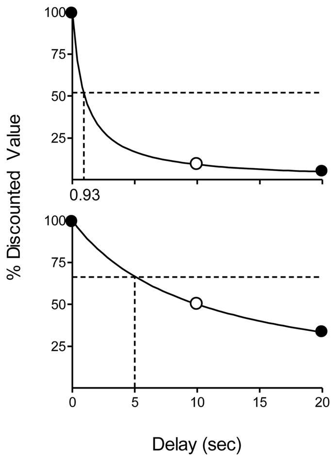
Discounting functions drawn using k-values of 1.0 (top panel) and 0.1 (bottom panel). The discounted value of the mixed-delay (gambling-like) arrangement is given by the horizontal dashed line in each panel. The vertical dashed lines show the indifference delay (i.e., the fixed delay at which the mixed- and fixed-delay alternatives have the same discounted value).
The bottom panel of Figure 1 illustrates why, according to Equation 2, steep delay discounting is correlated with pathological gambling. This panel shows the same delays to reinforcement but the delay discounting function is less steep (k = 0.1). As above, the discounted value of the reinforcers obtained from the MD 10-s schedule (horizontal dashed line) exceeds that of the FD (open data point), but the difference in value is less extreme than in the top panel. Thus, steep delay discounting means that the discounted value of a MD reward will greatly exceed that of a FD reward. More-shallow discounting renders the discounted value of the MD reward nearer to the FD alternative.
The predictions of Equation 2 also apply to the unpredictable delays indigenous to gambling games such as slot machines. To illustrate, we programmed a computer to repeatedly gamble until it had won 200,000 times. The odds of winning were set at 1 in 100 and the amount of each win was 100. To apply Equation 2 to this simulation we calculated Vu by a) equating Di with the numbers of losses before each win, b) determining the obtained probability of experiencing each of these delays (Pi), and c) setting A to 100.
Next, we used Equation 2 to calculate the discounted value of a reward of the same amount delivered following a predictable delay of 100 units (equivalent to the average delay experienced by gambling). Finally, we calculated the percent increase in subjective value that could be obtained by choosing the unpredictably over the predictably delayed reinforcer. We did this at nine different values of k. As illustrated in Figure 2, there is little to be gained by gambling when k is low, but as k increases, the subjective value of unpredictably delayed gambling-like rewards greatly exceeds that of the predictably delayed alternative.
Figure 2.

Hypothesized relation between steepness of the discounting curve (k) and the percent increase in subjective reward value that may be obtained by forgoing predictably delayed (non-gambling) rewards in favor of unpredictably delayed gambling-like rewards. Shaded area corresponds to the range of k-values reported for individuals diagnosed with pathological gambling. Solid line shows predictions for pathological gamblers with a history of a substance use disorder (k = 0.29).
The shaded area between dashed lines in Figure 2 shows the range of k values reported in studies of pathological gamblers not diagnosed with a substance-use disorder (k = 0.031–0.06; Madden et al., 2009; Petry, 2001); Ledgerwood et al. (2009) did not report k values so their data were not included in this range. For pathological gamblers, based on the values used in our computer simulation, Equation 2 predicts that unpredictably delayed rewards are subjectively worth at least 51% more than predictably delayed rewards. The solid line in Figure 2 (k = 0.29) suggests that unpredictably delayed rewards are even more alluring to individuals diagnosed with pathological gambling and with a prior history of substance use (Petry). As noted above, Alessi and Petry (2003) reported that among human pathological-gamblers, steeper delay discounting was associated with severity of the gambling disorder (as measured by the SOGS). Equation 2 provides a quantitative model that predicts this association.
Given these findings and analyses, the present study was conducted to evaluate Equation 2 by determining if steep delay discounting is correlated with the strength of preference for MD over FD alternatives. Delay discounting was measured in the first condition by assessing impulsive choices at four different delays to a larger-later food reward. Rats that made choices that were systematically affected by delays and were not biased toward one lever continued in the study. The second condition was designed to quantify the relative discounted values of MD and FD rewards. This was accomplished by giving rats a choice between food delivered after a MD or an adjusting FD (FD value was adjusted between sessions until stable indifference was obtained). Equation 2 predicts that the FD value at indifference (referred to henceforth as the indifference delay) will be inversely related to impulsive choice. This is illustrated by the vertical dashed lines in Figure 1. In the top panel, the discounted value of the FD reward crosses the horizontal line (discounted value of the MD reward) at an indifference delay of 0.93 s. At a lower k-value (bottom panel of Figure 1) the predicted indifference delay (5.01 s) is much higher.
Method
Subjects
Fifteen male Wistar rats (Harlan, Indianapolis, IN) approximately 2.5 months old at the start of the experiment were used. Rats were selected from a larger group that completed an impulsivity assessment (described below). The rats selected were those that made choices systematically affected by delay and not substantively biased toward one lever over the other. Rats were weighed daily and maintained at approximately 85% of their free-feeding weights through supplemental, post-session feeding provided at least 2 hr after each session. Between sessions, rats were housed individually in plastic cages within a temperature-controlled colony room providing a 12:12 hr light/dark cycle. Sessions were conducted during the light portion of the cycle. Water was continuously available between sessions.
Apparatus
Twelve identical operant chambers (Med Associates, St. Albans, VT), each measuring 24.1 cm wide, 30.5 cm long, and 21 cm high, were used. One wall of the chamber was an intelligence panel equipped with a non-retractable center lever (11 cm above the floor) and two retractable side levers (horizontally aligned 11 cm apart and 6.5 cm above the floor). Above each lever was a white, 28-volt DC cue light (2.5 cm in diameter and 6 cm above each lever). A feeder (Coulbourn, Allentown, PA) delivered 45-mg grain-based food pellets (BioServ, Frenchtown, NJ) into a receptacle (3 cm wide and 4 cm long) equipped with a 2-W light in the center of the intelligence panel (1 cm above the floor and 10 cm below the center lever). All feeders were outfitted with infrared pellet detectors to insure integrity of pellet delivery (Pinkston et al., 2008). Chambers were enclosed within a light- and sound-attenuation cubicle (Med Associates ENV-018MD) equipped with a ventilation fan and a white noise speaker. A Med Associates interface system controlled the sessions and collected data.
Procedure
Pretraining
An autoshaping program was used to train separately pressing of each of the three levers. Once responding was established, rats were exposed to ten 100-trial sessions during which a response on a lit center lever extinguished the center cue light, and caused the insertion of one of the side levers and the illumination of the cue light above the inserted lever. A response on the side lever retracted the lever, turned off the cue light, and delivered one food pellet. Side levers were presented in a strictly alternating pattern.
Condition 1: Impulsivity assessment
Sessions were composed of 42 trials, organized into seven blocks of 6 trials. Each block consisted of four forced-choice trials (two on the left lever and two on the right) followed by two free-choice trials. Within each block, the order of forced-choice trials was randomized without replacement. The illumination of the center cue light signaled the start of every trial. On forced-choice trials, a response on the center lever extinguished the cue light and caused the simultaneous insertion of one side lever and onset of the cue light above the inserted lever. A single response on the side lever retracted the lever and initiated the pellet delivery sequence. On forced- smaller-sooner (SS) reinforcer trials, the cue light was extinguished and one food pellet was delivered immediately. On forced-larger-later (LL) reinforcer trials, the cue light flashed in 0.25-s intervals during a delay to the delivery of three pellets. A flash of light in the food receptacle accompanied the delivery of each pellet. On free-choice trials, the procedure was identical except that both side levers were simultaneously inserted into the chamber and the cue light above each was illuminated. As during forced-choice trials, a single side-lever response initiated the corresponding SS or LL pellet-delivery sequence.
Pellet deliveries were followed by an inter-trial interval (ITI) during which no stimuli were presented. The duration of the ITI was adjusted such that each trial started after exactly 100 s, regardless of lever selection or response latency. Within each trial, a limited hold of 30 s was in effect – if a center-lever or side-lever response took longer than 30 s, the trial ended, the ITI was initiated, and an omission was scored.
The sequence of delays to the LL reinforcer was 5, 10, 15, and 0 s. Delays remained in effect for 30 sessions. At each delay, the LL reinforcer was assigned to either the left or right lever for 15 sessions, and then on the opposite lever for the remaining 15 sessions. Initial lever assignment was counterbalanced across rats.
Mean percent choice of the LL reinforcer at each delay was calculated using the last four sessions at each lever assignment (i.e., 8 sessions contributed to the mean). Choice was plotted as a function of delay and the area under the preference function (AUC) was used as a quantitative index of delay discounting (Madden et al., 2008). It should be noted that although these AUC values are expressed in normalized units, the data from which they were derived are not indifference points and, therefore, should not be compared to AUC values calculated from experiments using adjusting-amount or adjusting-delay procedures (Myerson et al., 2001).
Condition 2: Mixed-vs. fixed-delay choice
In this condition, rats chose between MD and FD schedules of food rewards. Two MD values were examined (10 and 30 s, in that order) because Equation 2 predicts the positive relation between AUC and indifference delays should increase with MD value (see Appendix). The MD schedules were composed of two values (0.01s and either 20 s [MD 10 s] or 60 s [MD 30 s]). The FD value was adjusted between sessions until a stable indifference delay was reached (i.e., the FD at which stable indifference was achieved between the MD and FD alternatives). The MD alternative was assigned to the lever most recently associated with the SS reinforcer in Condition 1 and was not changed during Condition 2.
Sessions were composed of 72 trials, organized into nine 8-trial blocks. Each block started with 4 forced-choice trials (random sequence, two on each lever) followed by 4 free-choice trials. With three exceptions, the sequence of within-trial events was as in Condition 1. First, pressing a side lever initiated either an MD or FD to two food pellets. If the MD lever was selected, the delay (0.01 or 20 s) was randomly selected, with replacement. Pressing the FD lever initiated a fixed-duration delay that was unchanged within-session. Second, regardless of the lever selected, the cue light above the retracted lever was constantly illuminated during the delay. Third, the ITI was set to 60 s.
The direction of between-session FD adjustment depended on the rat’s free-choices in the preceding session. If the MD alternative had been selected on > 60% of free-choice trials, then the FD was decreased by 2 s prior to the next session. If the MD alternative was selected < 40% of the time, the FD was increased by 2 s. After the 20th session of Condition 2, adjustments to the FD were made in 1-s increments. No adjustment was made to the FD if the MD alternative was chosen on 40–60% of the free-choice trials in the preceding session.
A stable indifference delay was achieved when the adjusted FD value and the percent choice of the MD alternative stabilized according to the following criteria: (a) the mean of the last six sessions was not the highest or the lowest six-session mean of the condition; (b) the mean of the last three sessions did not differ from the mean of the preceding three sessions by more than 2 s (FD) or 15% (MD choice); and (c) no monotonic trend was observed over the last six sessions.
Reassessment of impulsive choice
After stability was achieved at the final MD value of Condition 2, percent impulsive choice was reassessed for 30 sessions at the 10-s delay (15 sessions with the larger-later alternative programmed on the left and right sessions). This delay was selected because it was a delay at which choice was differentiated between rats; thus allowing an assessment for possible changes in impulsive choice occurring over time or as a result of experience with Condition 2.
Results & Discussion
Figure 3 shows the mean percent choice of the LL reinforcer at delays ranging from 0 to 15 s (see also Table 2); group means are shown as horizontal lines. At the 0 s delay, all rats nearly exclusively preferred the larger number of pellets. At the 10 s delay, two groups of rats are discriminable; 6 rats preferred the SS reinforcer, whereas the remaining 9 were still most often selecting the LL one. Larger individual differences were observed at the 15 s delay.
Figure 3.

Individual rats’ percent choice of the larger-later (LL) reinforcer as a function of LL delay. Group means are represented by horizontal lines.
Table 2.
Results of Conditions 1 and 2. Asterisks indicate experienced rats.
| Condition 1: Mean % LL Choice (SEM) | Cond 2: MD/FD 10s | Cond 2: MD/FD 30s | |||||||
|---|---|---|---|---|---|---|---|---|---|
| Rat | 0s | 5s | 10s | 15s | AUC | Indifference Delay | Sessions | Indifference Delay | Sessions |
| R1B1 | 100 (0) | 99.1 (0.9) | 98.2 (1.2) | 97.3 (1.3) | 0.99 | 7.3 | 66 | 5.8 | 113 |
| B1Br3 | 100 (0) | 97.0 (1.5) | 95.6 (1.9) | 97.3 (1.3) | 0.97 | 2.2 | 27 | 7.7 | 35 |
| G1Br2 | 100 (0) | 98.2 (1.2) | 94.7 (2.2) | 90.2 (5.0) | 0.96 | 7.2 | 77 | 8.3 | 25 |
| Br1B2 | 100 (0) | 98.2 (1.2) | 94.7 (2.2) | 75.9 (9.4) | 0.94 | 5.0 | 41 | 5.8 | 69 |
| G1B4 | 100 (0) | 100 (0) | 88.4 (4.5) | 81.2 (8.4) | 0.93 | 0.17 | 90 | 5.67 | 90 |
| Bl1B4 | 99.1 (0.9) | 95.3 (2.1) | 94.7 (2.9) | 53.6 (7.5) | 0.89 | 3.7 | 80 | 10 | 37 |
| R1B3 | 100 (0) | 98.2 (1.2) | 78.6 (7.1) | 64.3 (11.9) | 0.86 | 4.3 | 53 | 11 | 20 |
| Bl1B1 | 100 (0) | 93.8 (3.1) | 90.2 (3.3) | 35.7 (7.0) | 0.84 | 5.3 | 27 | 7.3 | 31 |
| B1Bl1 | 100 (0) | 96.5 (1.3) | 85.7 (5.5) | 35.7 (11.4) | 0.83 | 0.1 | 89 | 15.2 | 29 |
| G1Br3 | 100 (0) | 94.7 (2.6) | 18.7 (6.3) | 20.5 (7.2) | 0.58 | 4.5 | 112 | 7.7 | 31 |
| B1Br4 | 100 (0) | 95.5 (1.9) | 11.6 (8.6) | 22.3 (7.9) | 0.56 | 4.3 | 69 | 4.7 | 36 |
| Br1B1 | 99.1 (0.9) | 95.5 (1.9) | 3.6 (2.7) | 32.1 (12.4) | 0.55 | 2.2 | 34 | 5.8 | 80 |
| G1Br1 | 99.1 (0.9) | 60.7 (8.3) | 29.4 (9.3) | 8.0 (3.4) | 0.48 | 3.5 | 64 | 6.0 | 54 |
| B1Br1 | 98.2 (1.1) | 79.5 (7.1) | 8.0 (1.6) | 4.4 (2.7) | 0.46 | 3.3 | 20 | 9.8 | 98 |
| Br1B3 | 100 (0) | 50 (9.9) | 9.8 (3.3) | 2.7 (1.3) | 0.37 | 4.0 | 59 | 6.7 | 35 |
The top panel of Figure 4 shows the correlations between AUC values and indifference delays obtained in Condition 2. Kolmogorov-Smirnov tests indicated that the distributions were Gaussian, therefore Pearson correlation coefficients are shown. Neither correlation approached significance; therefore, the prediction of Equation 2 was not supported. Two rats’ stable indifference delays in the MD 10-s portion of Condition 2 were < 0.2 sec, which suggests a side bias. When these indifference points were removed from the scatterplot, the correlation in this portion of Condition 2 approached significance (r = .44, p=.07).
Figure 4.

Top: Correlations between stable indifference delays and area under the curve (AUC). Separate regression lines and data points are presented for the two mixed-delay (MD) values. Bottom: Percent change in LL choice from the 10-s delay portion of Condition 1 to the reassessment at the same delay. Positive deviations less than zero indicate a shift toward more LL choices.
The bottom panel of Figure 4 shows the change in percent LL choice from the 10-s delay portion of Condition 1 to the post-Condition 2 reassessment at the same delay. A significant change toward fewer impulsive choices was observed (one-sample t(15)=2.55, p < .05), with 6 rats’ choices shifting in this direction by at least 25%. The latter rats are those in the upper panel of Figure 4 with AUC values less than 0.6. This shift bears formal similarity to the age-related decrease in delay discounting reported in a cross-sectional study of 6- and 24-month old rats by Simon et al. (2010). While the decrease in impulsive choice observed in our study may be age related, the span of time separating Condition 1 and the post-Condition 2 reassessment averaged only 108 days (115 days for the 6 rats with the largest changes in impulsive choice). Until more fine-grained measures of delay discounting are explored across the lifetime, it will be difficult to attribute the impulsivity shifts observed here to aging alone.
A second possibility is that experience with the delays arranged in Condition 2 is responsible for the decrease in impulsive choice. Prior experiments that have experimentally decreased impulsive choice in pigeons have included extensive exposure to reinforcer delays (e.g., Logue, Rodriguez, Pena-Correal, & Mauro, 1984; Mazur & Logue, 1978). In Condition 2 of the present study, even those rats that strongly preferred the MD alternative were exposed to 20- and 60-s delays on many trials for over 100 sessions. This experience may have decreased sensitivity to reinforcer delay. If so, then a critical premise in evaluating the relation between impulsive choice and strength of preference for an MD over a FD alternative was violated: that the degree of impulsive choice quantified in Condition 1 would be stable over Condition 2. With the observed shift toward fewer impulsive choices, the individual differences needed to detect a relation between delay discounting and strength of preference for MD over FD rewards evaporated.
Although the present study does not support the prediction of Equation 2, a more definitive test must await the results of a study in which delay discounting does not change from pre- to post assessments. A pilot study conducted in our lab suggests that this more definitive study is worth pursuing. In the pilot study, 5 rats twice completed Condition 1 (as described above). Between the first and second assessment of impulsivity, AUC changed by an average of 0.2% (range: −9.25 to 9.5%). Next, these rats earned food reinforcers on ratio schedules for 180 days; after which LL choice was reassessed at the 10-s delay and found to have changed from the preceding assessment by an average of −3.9 % (range: −20.5 to 17%). These rats then completed Condition 2, achieving the stable indifference delays shown in Figure 5 (AUC values are those obtained in the second exposure to Condition 1). The significant correlations between AUC and stable indifference delays are in the direction predicted by Equation 2.
Figure 5.

Correlations between stable indifference delays and area under the curve (AUC). Separate regression lines and data points are presented for the two mixed-delay (MD) values. Data are from a pilot study of 5 rats.
These correlations should be interpreted in light of what they are: pilot data. The sample size is very small, two rats’ indifference points in the MD 30 s portion of Condition 2 were suggestive of a side bias, and impulsive choice was not reassessed after Condition 2; thus, impulsivity may have shifted during Condition 2 as it did for the previous group of 15 rats. Nonetheless the data suggest that a more systematic examination of the prediction of Equation 2 is worth pursuing. Selecting for stable individual differences in AUC is one method by which this might be approached, but another is to decrease the duration of Condition 2. Lagorio and Hackenberg (2010) reported orderly data in an experiment similar to Condition 2, but they adjusted the duration of the FD within-, rather than between-sessions. Under conditions comparable to our Condition 2, stable indifference delays were obtained in their study in approximately half the number of sessions.
A final possible reason that our measure of delay discounting, AUC, was not correlated with strength of preference for mixed- over fixed-delays is that AUC may have been affected by sensitivity to reinforcer amount. Equation 2 holds that strength of preference for variable delays is determined by the shape of the discounting curve and sensitivity to reinforcer delay alone. In Condition 2, the amount of the MD and FD reinforcers was identical; however in Condition 1, subjects chose between reinforcers that differed in amount and delay. If individual differences in AUC were due in part to differences in sensitivity to reinforcer amount, then the lack of a correlation between AUC and indifference delays would not be surprising. Future studies may benefit by quantifying sensitivity to reinforcer delay using a concurrent-chains generalized matching law analysis (e.g., Logue et al., 1984) instead of the assessment of impulsive choice used here. Until that time, the prediction of Equation 2 will remain quantitatively sound, but without empirical support.
Acknowledgments
The authors thank Shannon Tierney and Gabriella Yates for their technical assistance. This research was supported by NIH grants 1R21DA023564 and 1R01DA029605 awarded to the first author.
Appendix
Equation 2 predicts that as the MD value increases from 10 to 30 s, the effect of k on the predicted FD value at which choice stabilizes at indifference (i.e., the indifference delay) will increase.
| k | MD | V | Predicted Indifference Delay | Difference |
|---|---|---|---|---|
| 0.3 | 10 | 1.14 pellets | 2.5 s | 1.9 s |
| 1.5 | 10 | 1.03 pellets | 0.6 s | |
| 0.3 | 30 | 1.05 pellets | 3 s | 2.4 s |
| 1.5 | 30 | 1.01 pellets | 0.6 s |
Footnotes
Unlike string theory, Equation 2 does not include an explicit parameter for losses. Losses factor into Equation 2 only to the extent that a loss delays the delivery of the gambling win. This may be a reasonable assumption if the amount of the loss is unchanging between wagers (each loss adds a constant amount to Di), but the equation is silent about the effects of different magnitude losses on decision making. If the predictions of Equation 2 hold when losses are constant (e.g., the labor lost by each unreinforced lever press in the present experiment), the generality of the equation to human gambling may require the addition of a factor representing loss amount.
Publisher's Disclaimer: This is a PDF file of an unedited manuscript that has been accepted for publication. As a service to our customers we are providing this early version of the manuscript. The manuscript will undergo copyediting, typesetting, and review of the resulting proof before it is published in its final citable form. Please note that during the production process errors may be discovered which could affect the content, and all legal disclaimers that apply to the journal pertain.
References
- Alessi SM, Petry NM. Pathological gambling severity is associated with impulsivity in a delay discounting procedure. Behav Processes. 2003;64:345–354. doi: 10.1016/s0376-6357(03)00150-5. [DOI] [PubMed] [Google Scholar]
- American Psychiatric Association. Diagnostic and Statistical Manual of Mental Disorders. 4. American Psychiatric Association; Washington DC: 1994. [Google Scholar]
- Carroll ME, Anker JJ, Mach JL, Newman JL, Perry JL. Delay discounting as a predictor of drug abuse. In: Madden GJ, Bickel WK, editors. Impulsivity: The Behavioral and Neurological Science of Discounting. American Psychological Association; Washington, DC: 2010. pp. 243–271. [Google Scholar]
- de Wit H, Mitchell SH. Drug effects on delay discounting. In: Madden GJ, Bickel WK, editors. Impulsivity: The Behavioral and Neurological Science of Discounting. American Psychological Association; Washington, DC: 2010. pp. 213–241. [Google Scholar]
- Dixon MR, Jacobs EA, Sanders S. Contextual control of delay discounting by pathological gamblers. J Appl, Behav Anal. 2006;39:413–422. doi: 10.1901/jaba.2006.173-05. [DOI] [PMC free article] [PubMed] [Google Scholar]
- Dixon MR, Marley J, Jacobs EA. Delay discounting by pathological gamblers. J Appl, Behav Anal. 2003;36:449–458. doi: 10.1901/jaba.2003.36-449. [DOI] [PMC free article] [PubMed] [Google Scholar]
- Gerstein D, Murphy S, Toce M, Hoffmann J, Palmer A, Johnson R, Larison C, Chuchro L, Buie T, Engelman L, Hill MA. Gambling Impact and Behavior Study. University of Chicago Press; Chicago, IL: 1999. [Google Scholar]
- Holt DD, Green L, Myerson J. Is discounting impulsive? Evidence from temporal and probability discounting in gambling and non-gambling college students. Behav Processes. 2003;64:355–367. doi: 10.1016/s0376-6357(03)00141-4. [DOI] [PubMed] [Google Scholar]
- Kacelnik A, Bateson M. Risky theories the – effects of variance on foraging decisions. American Zoologist. 1996;36:402–434. [Google Scholar]
- Kirby KN, Maraković NN. Modeling myopic decisions: Evidence for hyperbolic delay-discounting within subjects and amounts. Org Behav and Human Decision Processes. 1995;64:22–30. [Google Scholar]
- Lagorio CH, Hackenberg TD. Risky choice in pigeons and humans: A cross-species comparison. J Exp Anal Behav. 2010;93:27–44. doi: 10.1901/jeab.2010.93-27. [DOI] [PMC free article] [PubMed] [Google Scholar]
- Ledgerwood DM, Alessi SM, Phoenix N, Petry NM. Behavioral assessment of impulsivity in pathological gamblers with and without substance use disorder histories versus healthy controls. Drug Alcohol Depend. 2009;105:89–96. doi: 10.1016/j.drugalcdep.2009.06.011. [DOI] [PMC free article] [PubMed] [Google Scholar]
- Lesieur HR, Blume SB. The South Oaks Gambling Screen (SOGS): A new instrument for the identification of pathological gamblers. Am J Psychiatry. 1987;144:1184–1188. doi: 10.1176/ajp.144.9.1184. [DOI] [PubMed] [Google Scholar]
- Locey ML, Pietras CJ, Hackenberg TD. Human risky choice: Delay sensitivity depends on reinforcer type. J Exp Psychol Anim Behav Process. 2009;35:15–22. doi: 10.1037/a0012378. [DOI] [PubMed] [Google Scholar]
- Logue AW, Rodriguez ML, Peña-Correal TE, Mauro BC. Choice in a self-control paradigm: Quantification of experience-based differences. J Exp Anal Behav. 1984;41:53–67. doi: 10.1901/jeab.1984.41-53. [DOI] [PMC free article] [PubMed] [Google Scholar]
- MacKillop J, Anderson EJ, Castelda BA, Mattson RE, Donovick PJ. Divergent validity of measures of cognitive distortions, impulsivity, and time perspective in pathological gambling. J Gamb Stud. 2006;22:339–354. doi: 10.1007/s10899-006-9021-9. [DOI] [PubMed] [Google Scholar]
- Madden GJ, Ewan EE, Lagorio CH. Toward an animal model of gambling: delay discounting and the allure of unpredictable outcomes. J Gamb Stud. 2007;23:3–83. doi: 10.1007/s10899-006-9041-5. [DOI] [PubMed] [Google Scholar]
- Madden GJ, Petry NM, Johnson PS. Pathological gamblers discounting probabilistic rewards less steeply than controls. Exp Clin Psychopharmacol. 2009;17:283–290. doi: 10.1037/a0016806. [DOI] [PMC free article] [PubMed] [Google Scholar]
- Madden GJ, Smith NG, Brewer AT, Pinkston JW, Johnson PS. Steady-state assessment of impulsive choice in Lewis and Fischer 344 rats: Between-session delay manipulations. J Exp Anal Behav. 2008;90:333–344. doi: 10.1901/jeab.2008.90-333. [DOI] [PMC free article] [PubMed] [Google Scholar]
- Mazur JE. An adjusting procedure for studying delayed reinforcement. In: Commons ML, Mazur JE, Nevin JA, Rachlin H, editors. Qualitative analyses of behavior: The effect of delay and of intervening events on reinforcement value. Erlbaum; Hillsdale, NJ: 1987. pp. 55–73. [Google Scholar]
- Mazur JE. Theories of probabilistic reinforcement. J Exp Anal Behav. 1989;51:87–99. doi: 10.1901/jeab.1989.51-87. [DOI] [PMC free article] [PubMed] [Google Scholar]
- Mazur JE, Logue AW. Choice is a self-control paradigm: Effects of a fading procedure. J Exp Anal Behav. 1978;30:11–17. doi: 10.1901/jeab.1978.30-11. [DOI] [PMC free article] [PubMed] [Google Scholar]
- Myerson J, Green L, Warusawitharana M. Area under the curve as a measure of discounting. J Exp Anal Behav. 2001;76:235–243. doi: 10.1901/jeab.2001.76-235. [DOI] [PMC free article] [PubMed] [Google Scholar]
- Odum AL, Madden GJ, Badger GJ, Bickel WK. Needle sharing in opioid-dependent outpatients: Psychological processes underlying risk. Drug Alcohol Depend. 2000;60:259–266. doi: 10.1016/s0376-8716(00)00111-3. [DOI] [PubMed] [Google Scholar]
- Petry NM. Pathological gamblers, with and without substance use disorders, discount delayed rewards at high rates. J Abnormal Psychol. 2001;110:482–487. doi: 10.1037//0021-843x.110.3.482. [DOI] [PubMed] [Google Scholar]
- Petry NM, Casarella T. Excessive discounting of delayed rewards in substance abusers with gambling problems. Drug Alcohol Depend. 1999;56:25–32. doi: 10.1016/s0376-8716(99)00010-1. [DOI] [PubMed] [Google Scholar]
- Petry NM, Madden GJ. Discounting and pathological gambling. In: Madden GJ, Bickel WK, editors. Impulsivity: The Behavioral and Neurological Science of Discounting. American Psychological Association; Washington, DC: 2010. pp. 273–294. [Google Scholar]
- Pinkston JW, Ratzlaff KL, Madden GJ, Fowler SC. An inexpensive infrared detector to verify the delivery of food pellets. J Exp Anal Behav. 2008;90:249–255. doi: 10.1901/jeab.2008.90-249. [DOI] [PMC free article] [PubMed] [Google Scholar]
- Rachlin H. Why do people gamble and keep gambling despite heavy losses? Psychol Science. 1990;1:294–297. [Google Scholar]
- Rachlin H, Raineri A, Cross D. Subjective probability and delay. J Exp Anal Behav. 1991;55:233–244. doi: 10.1901/jeab.1991.55-233. [DOI] [PMC free article] [PubMed] [Google Scholar]
- Setlow B, Mendez IA, Mitchell MR, Simon NW. Effects of chronic administration of drugs of abuse on impulsive choice (delay discounting) in animal models. Behav Pharmacol. 2009;20:380–389. doi: 10.1097/FBP.0b013e3283305eb4. [DOI] [PMC free article] [PubMed] [Google Scholar]
- Simon NW, LaSarge CL, Montgomery KS, Williams MT, Mendez IA, Setlow B, Bizon JL. Good things come to those who wait: Attenuating discounting of delayed rewards in aged Fischer 344 rats. Neurobiol Aging. 2010;31:853–862. doi: 10.1016/j.neurobiolaging.2008.06.004. [DOI] [PMC free article] [PubMed] [Google Scholar]
- Stinchfield R. Reliability, validity, and classification accuracy of the South Oaks Gambling Screen (SOGS) Addict Behav. 2002;27:1–19. doi: 10.1016/s0306-4603(00)00158-1. [DOI] [PubMed] [Google Scholar]
- Yi R, Mitchell SH, Bickel WK. Delay discounting and substance abuse-dependence. In: Madden GJ, Bickel WK, editors. Impulsivity: The Behavioral and Neurological Science of Discounting. American Psychological Association; Washington, DC: 2010. pp. 191–211. [Google Scholar]