Functional genetics of intraspecific ecological interactions in Arabidopsis thaliana

Abstract

Studying the genetic basis of traits involved in ecological interactions is a fundamental part of elucidating the connections between evolutionary and ecological processes. Such knowledge allows one to link genetic models of trait evolution with ecological models describing interactions within and between species. Previous work has shown that connections between genetic and ecological processes in Arabidopsis thaliana may be mediated by the fact that quantitative trait loci (QTL) with ‘direct’ effects on traits of individuals also have pleiotropic ‘indirect’ effects on traits expressed in neighbouring plants. Here, we further explore these connections by examining functional relationships between traits affected directly and indirectly by the same QTL. We develop a novel approach using structural equation models (SEMs) to determine whether observed pleiotropic effects result from traits directly affected by the QTL in focal individuals causing the changes in the neighbours' phenotypes. This hypothesis was assessed using SEMs to test whether focal plant phenotypes appear to mediate the connection between the focal plants' genotypes and the phenotypes of their neighbours, or alternatively, whether the connection between the focal plants' genotypes and the neighbours' phenotypes is mediated by unmeasured traits. We implement this analysis using a QTL of major effect that maps to the well-characterized flowering locus, FRIGIDA. The SEMs support the hypothesis that the pleiotropic indirect effects of this locus arise from size and developmental timing-related traits in focal plants affecting the expression of developmental traits in their neighbours. Our findings provide empirical insights into the genetics and nature of intraspecific ecological interactions. Our technique holds promise in directing future work into the genetic basis and functional relationship of traits mediating and responding to ecological interactions.

1. Introduction

One of the keys to bridging the connections between evolutionary and ecological processes is understanding the genetic basis of ecological interactions. This kind of knowledge allows one to link the micro- and macro-evolutionary genetic models at the heart of evolutionary biology with models of ecological interactions both within and among species. In this unified framework, patterns of genetic variation and covariation determine the evolutionary dynamics and reflect the nature of past selective pressures on traits involved in ecological interactions, while ecological interactions, in turn, govern evolutionary dynamics by determining the form and strength of selection acting on these traits. These ecology–evolution links underlie some of the most interesting questions in both fields, including those related to the evolution of competition (e.g. [1,2]) and the development of traits involved in processes such as niche construction [3]. Many related ecological interactions, such as competition and facilitation, have been shown to have a genetic basis [4–8] as have other broader processes at the community level such as community composition [9,10]. Further steps toward understanding connections between evolutionary and ecological processes can elucidate how evolution affects individuals interacting both within and between species. Ultimately, such information can improve our understanding of both natural and agricultural systems (e.g. [11]), yet there is surprisingly little known about the specific genetic basis underlying ecological interactions among individuals in a population.

In many species, the most important sources of ecological interactions are ‘social’ interactions between conspecifics (e.g. intraspecific competition; [12–14]). In these cases, the environment provided by conspecifics can have profound effects on the phenotype or fitness of individuals. These ‘social environments’ can arise from either direct behavioural interactions between individuals (e.g. [15]), non-behavioural traits expressed in conspecifics (e.g. [16,17]) or owing to degradation or alteration of the abiotic environment caused by neighbours that has an impact on other conspecifics [18–20]. Ultimately, through the social environment, a neighbour's traits may affect the expression of traits in a focal individual. In this way, social interactions can result in ‘social effects’ (also known as ‘associate effects’; [21]), where traits expressed in one individual affect traits expressed in other individuals (see [22]). These social effects provide the opportunity for ‘indirect genetic effects’ (IGEs) when genes in one individual affect the expression of traits in other individuals, and indirect environmental effects when environmental effects on trait expression in one individual result in changes in the expression of traits in other individuals [23]. Theory suggests that the IGEs arising from social interactions can potentially have large effects on the dynamics of trait evolution [23,24], and empirical studies have implicated IGEs in a number of intraspecific [5,10] and interspecific (see [22]) evolutionary and ecological processes. However, despite the fact that studies have begun to investigate the evolutionary and ecological genetics of IGEs, scant empirical evidence exists for the functional basis of how genetic variation in one individual maps to traits expressed in other individuals.

The theoretical framework underlying IGEs is based on ‘interacting phenotypes models’ ([23]; illustrated in figure 1a) and allows for the partitioning of genetic (g) and environmental (e) effects when trait expression is affected by interactions between individuals. In these models, the phenotype of one or more focal individuals (phenotype D in figure 1a) affects the expression of traits in an interacting partner or neighbour individual (phenotype I in figure 1a). As a result of these social effects on trait expression, genetic factors in one individual affect the phenotype of another individual or individuals, with this effect being mediated through the first individual's phenotype. Therefore, the interacting phenotypes model provides a formal structure for understanding these effects because it allows genotypes of one individual to be linked to phenotypes of other individuals via these interactions. In turn, this allows a better understanding of the functional origin of the IGEs and their possible effect on evolutionary dynamics. Although we focus on intraspecific interactions herein, this approach can be equally useful in interspecific interactions, where genes expressed in individuals of one species map to the phenotypes of individuals of other species via phenotypically mediated interactions (see [10]). Therefore, the framework we discuss here can be easily extended to consider the diversity of ecological interactions that occur within and between species.

Figure 1.

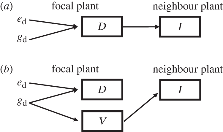
Indirect genetic effects (IGEs) arise from the mapping of the genotype of the focal individual to the phenotype of their neighbours. (a) The case where IGEs arise from the social effect of a focal plant's ‘direct trait’ (D) on the expression of a neighbour's ‘indirect trait’ (I). g_d denotes direct genetic effects where the focal individual's genotype maps to their (direct) phenotype. e_d denotes direct environmental effects, which are non-genetic effects on the focal individual's phenotype (i.e. the direct trait). The direct trait has a social/ecological effect on the expression of the indirect trait by neighbours (shown by the arrow from D to I). These social effects result in IGEs, illustrated by mapping from the focal genotype (g_d) to the neighbour's phenotype through the social effect of the direct trait on the indirect trait, and indirect environmental effects. Thus, in this scenario there is identified pleiotropy between direct and IGEs on traits D and I because the direct effect on trait D gives rise to the indirect effect on trait I (i.e. the effect is because of an identified/measured trait). (b) The case where there are IGEs of the focal individual's genotype on the neighbour's phenotype, but there is unidentified pleiotropy between traits D and I because there is no functional/causal connection between traits D and I. In this case, the indirect effect of the focal genotype on the indirect trait arises from the effect of an unmeasured trait (V) in the focal individual.

In previous work [8], we used a quantitative trait locus (QTL)-based approach in an experimental population of A. thaliana to identify the genetic basis of IGEs resulting from ecological interactions between neighbouring plants. We found not only a number of QTL underlying IGEs, but also that many suites of traits in the focal plants were pleiotropically linked with traits expressed by their neighbour plants (i.e. both were affected by the same QTL). However, it was not possible to establish whether the pattern of pleiotropy that we found was owing to (or closely tied to) the measured traits in focal individuals affecting the traits expressed in the neighbours (figure 1a), or, in contrast, whether the pleiotropy was caused by some unmeasured traits (illustrated in figure 1b). The interacting phenotypes framework implies that IGEs must ultimately be caused by traits in focal individuals that affect the expression of traits in their neighbours [25], and so the appearance of functional pleiotropic links between traits expressed in interacting individuals would be expected if the correct traits (i.e. the traits involved in the interaction) have been measured. However, traits may show pleiotropy if the traits expressed in interacting individuals are affected by the same locus but the two have no direct causal link, perhaps owing to a shared pleiotropic connection to some other unmeasured trait (see trait V in figure 1b).

To address the question of how genetic variation in the traits of one individual maps to trait variation in other individuals through functional relationships, we apply the theoretical framework of interacting phenotypes to a statistical analysis of social effects in the A. thaliana system, where IGEs have been previously documented [8]. We use path analysis to test for these functional relationships, because it can be used to describe and test hypotheses about directional relationships between variables. Path analysis has been used successfully to examine ecological [26,27] and evolutionary [28,29] relationships and fits well with the interacting phenotypes framework, which is built conceptually on path models [23]. However, in complex systems, with many traits spanning multiple individuals, there are so many possible relationships between traits expressed in interacting individuals that it is useful to look for relationships within individuals before examining any causal relationships between them owing to interactions. Factor analysis provides a system to summarize interactions by describing how sets of measured traits (e.g. leaf number, leaf size, plant height) form a single functional trait (e.g. ‘light gathering’ [30]). When used in conjunction, path and factor analysis are termed structural equation models (SEMs) and are extremely powerful in these complex situations. In our system, they allow for the testing of directional relationships between focal and neighbour populations as well as allowing for the association of many traits into a single composite trait (see figure 2 for various alternative model structures). Thus, using SEMs we can better understand how genotype makes phenotype within the individual, in terms of the relationship between traits, how traits within individuals together represent some ‘hidden’ traits, like resource pool or life-history strategy, and how features of one individual (genes, traits, hidden or measured) impact neighbours. While SEMs have been successfully implemented in ecological analyses such as studies of natural selection [29] and in QTL mapping [31,32], they have rarely been used to examine the nature of relationships between phenotypes (e.g. [33]), and have not previously been used to understand the genetics of ecological interactions.

Figure 2.

Examples of structural equation models (SEMs) for phenotypic interactions underlying indirect genetic effects. Each box represents a measured variable: G, the QTL genotype of the focal plant; D_n, the direct or focal plant traits; I_n, the indirect or neighbour plant traits. Each oval represents a latent variable or factor formed by the variables whose arrows are directed outward from the variable: L_D, a direct or focal plant trait factor; L_I, an indirect or neighbour plant trait factor. (a) Simple model where there is a direct latent variable composed of focal plant traits that influence some indirect trait. This is analogous to the indirect trait being incorporated into the direct latent factor. (b) The case where a host of focal plant traits (D_1–3) form a latent factor, which influences a neighbour plant factor, formed by its traits (I_1–3). Finally, (c) a case where a neighbour factor is affected by some of the focal plant traits, but not all. Each of these models is considered an ‘unidentified pleiotropy’ model, and can be reduced to an ‘identified pleiotropy’ model by removing the path from G to the indirect trait or factor.

Here, we use the SEM method to explicitly examine the functional basis to the pleiotropic relationship between the direct and indirect effects of QTL identified by Mutic & Wolf [8]. In doing so, we ask whether the variation in measured and composite traits of our focal plants appears to be the cause of variation in the expression of traits by neighbour plant traits, thereby linking the direct effects of the QTL on focal plant traits to their indirect effects on neighbour plant traits. We view our analysis as an illustration of a more general framework, and it is our hope that this general framework may be used more broadly to understand how IGEs link evolutionary and ecological processes.

2. Material and methods

(a). Experimental design

Details of the original experimental design are given in [8]. Briefly, our focal population is the set of 411 recombinant inbred lines (RILs) produced by crossing the natural accessions of Arabidopsis thaliana Bay-0 and Shahdara [34]. Each RIL was grown in a 2.5 cm pot with a standard neighbour genotype, the accession Ler-0. These pots were placed in the ‘ArabiPatch’ system (Lehle Seeds, Round Rock, TX, USA), which holds a set of eight pots, each fitted with a 30.5 cm tall tube to create a self-contained space for the pair of plants to grow and interact. We measured several traits at 42 days from planting in order to gather information related to plant development, size and fecundity. These traits included bolting time (BOLT), height (HT), flower number (FLWR), bud number (BUD), silique number (SILIQ), leaf number (LEAF), number of branches in the whole inflorescence (BRANCH) and dry weight (WT). Traits measured in the Ler partner plants are labelled with a ‘p’ prefix to denote ‘partner’ traits, while traits measured in the focal plants do not have a prefix. Table 1 provides a list of traits with their abbreviations for reference.

Table 1.

Patterns of effect of the QTL of major effect. Traits measured in the focal population (the Bay-0 × Shahdara RIL set) appear under the heading of ‘direct traits’ and those in the Ler partner plants appear as ‘neighbour (indirect) traits’. The abbreviations used in the text as labels for each trait are given next to the trait name. For each trait, the LPR score (where LPR = –log₁₀[p]), model R2 (% of variance explained), effect (with standard error) and standardized effect (effect/trait standard deviation) are given.

trait	LPR score	r2	effect	s.e.	standardized effect
direct traits
height (HT)	17.46	0.19	+62.64	6.72	+0.45
weighta (WT)	3.45	0.03	+1.34	0.37	+0.19
boltb (BOLT)	7.23	0.08	−0.048	0.0087	−0.29
budsa (BUD)	6.63	0.07	+0.40	0.075	+0.27
flowersa (FLWR)	11.65	0.13	+0.52	0.071	+0.37
siliquesa (SILIQ)	18.90	0.20	+1.21	0.13	+0.46
branchesa (BRANCH)	11.02	0.12	+0.26	0.037	+0.35
leaves (LEAF)	9.71	0.11	+0.99	0.15	+0.33
neighbour (indirect) traits
pBudsa (pBUD)	4.45	0.04	+0.30	0.071	+0.24
pFlowersa (pFLWR)	3.63	0.03	+0.23	0.028	+0.21
pBranchesa (pBRANCH)	2.88	0.03	+0.092	0.028	+0.18
pLeaves (pLEAF)	1.80	0.02	+0.25	0.104	+0.14

^aTraits were square-root transformed.

^bTrait was natural log-transformed.

(b). Quantitative trait loci mapping

In order to pursue a functional analysis of interactions involving the population presented in Mutic & Wolf [8], we started by re-doing the analysis of direct and indirect effects of QTL. Although it might make logical sense simply to use the results from Mutic and Wolf as the foundation for the present analysis, the analysis was redone for several reasons. Firstly, it was decided that the analysis would perform better if traits were transformed to normality or near normality (see below), as most traits showed some skew that could alter the performance of the models (SEMs can be very sensitive to deviations from multivariate normality). Secondly, the set of ‘late’ traits from our previous work was not included in this analysis because the sample size was smaller, and SEM analyses (described below) are highly sensitive to sample size.

The re-analysis followed the same approach as described in Mutic and Wolf, which used a regression model to locate QTL (implemented in the CANCORR procedure in SAS; SAS Institute, Cary, NC, USA) (see [35,36]). Genotypes were assigned the index values of +1 and −1 for the Bay-0 and Shahdara homozygotes at a locus, respectively, Therefore positive allelic effects can be interpreted as the effect of replacing the Shahdara allele with the Bay-0 allele [34]. Because of deviations from normality, we natural log-transformed BOLT and square root-transformed WT, BUD, FLWR, SILIQ and BRANCH for both the focal and partner traits. Because the analyses presented here are focused on the SEM analysis of QTL effects, we include only the relevant results of the QTL analysis as a component of the methods. The analysis of the transformed variables showed essentially the same results as the analyses presented in Mutic & Wolf [8], but with most logarithmic probability ratio (LPR) scores being larger than in the original analysis (i.e. QTL effects are stronger in the new analysis based on transformed traits). The LPR scores are the negative logarithm (base 10) of the probability values for the tests of QTL effects. They are comparable with logarithm of odds (LOD) scores typically seen in QTL analyses. For example, an LPR value of 5 corresponds to a probability of 10⁻⁵.

(c). Focal locus choice

Many of the QTL identified by Mutic and Wolf explain a very small proportion of the phenotypic variance in the focal population (e.g. 2–4%), and, because the indirect effects of the loci were always weaker than the direct effects, they explained proportionally less variation in the partner plants (generally 1–2%). Therefore, our goal was to avoid pursuing a functional analysis at loci that explained a very small proportion of phenotypic variance and focus our attentions on loci with strong clear patterns of effect. To obtain enough power to use SEMs to pursue functional relationships between traits in the focal and neighbour plants and their association with QTL, it is important to use loci that show relatively strong direct and indirect effects. Thus, to allow strong inferences to be made from the analysis, rather than just parsing subtle alternatives, we choose to perform the functional analysis on a single locus of large effect: QTL 4.02 (located at ca. 2cM on chromosome 4; see [8]; table 1). QTL 4.02, located at the start of chromosome 4, was chosen because it shows a major effect on several traits, and shows much stronger indirect effects than any other QTL (see §3).

(d). Model building and rationale

To determine whether the observed pattern of pleiotropy found for QTL 4.02 was attributable to measured traits in focal individuals affecting the traits expressed in the neighbours (what would be called ‘identified pleiotropy’, figure 1a), or whether it was caused by some unmeasured traits (‘unindentified pleiotropy’, figure 1b), we used SEMs to examine the influences of focal plant phenotypes on neighbouring plants. Conducting a blind search for all possible interacting traits in focal and partner plants is not feasible given the very large number of trait pairs and would probably yield many false-positive interactions. We developed a method similar to Li et al. [33] to avoid blindly searching for interactions between traits. First, we performed path analyses to examine relationships between the QTL and the sets of traits it pleioptropically affected. We then used those traits and the QTL to form more functional models that described the relationships between phenotypes, and interactions that had a genetic basis. We used the AMOS program (SPSS, Chicago, IL, USA) to perform all of our analyses.

We stress that the building of SEMs is a process of hypothesis development and testing. Because model structures can be complex and there can be a near-infinite number of alternative model structures, model building is inherently exploratory in nature, with no single established optimal approach. Our goal is to determine the model that best describes the pattern of the genotype–phenotype relationship and how interactions between individuals mediate that relationship. This is towards the broader goal of testing the hypothesis that the traits we measured are involved in the interaction between neighbouring plants.

Our approach to building an SEM can be divided into five steps:

1. Conduct a series of path analyses between focal and neighbour traits. This first step of our SEM building is a biologically meaningful way to screen the interactions for the final model. We conducted path analyses in which paths were made pair-wise to link all traits in the focal plant to all traits in the neighbour plant. We evaluated the significance of each path in the analysis and eliminated any that were not significant. To avoid spurious effects that could arise from environmental covariances between neighbours, we used partial regressions to examine the effect of both the marker and the focal plant trait on neighbours together. Note, however, that although environmental covariances can lead to associations between the phenotypes of neighbours, they are not expected to lead to associations in the next steps between QTL in the focal plants and the expression of traits in their neighbours (i.e. they should not affect this ‘causal’ path). Furthermore, the environmental covariances between neighbours are diminished in our study because we replicated the pairs and have used means of the replicates in our analyses (environmental covariances should lead to associations between the phenotypes of plants grown together, but not so much between the average phenotype of one group and the average phenotype of that group's partners). This test also provides the criteria to determine whether the inclusion of focal plant traits in the model affected the significance of the QTL-to-neighbour trait mapping. If the relative strength of the associations between QTL and neighbour traits was stronger than the focal trait–neighbour traits, the interaction was not included in further analyses because it indicated that any interactions were probably caused by traits that we did not measure.

Importantly, we also included covariances between error terms, which can help account for the environmental covariance that impacts the associations between traits. Accounting for correlated error terms can thus improve model construction by more accurately describing the relationships between traits [37], and including these covariances can increase power by explaining more error variance among traits.

2. Create more manageable, reduced models by eliminating insignificant interactions involved with the neighbour plant traits. We reduced our model further by removing non-significant covariances added in step 1. This is not a simple process of removing all non-significant terms from the model because each change to the path models has the potential to affect all other parameters, so this was an iterative step. Steps 1 and 2 were combined in AMOS by examining ‘modification indices’ that indicate paths that will improve or detract from model fit, but are detailed separately here for clarity.

3. Use the path analysis model as a starting point for making an SEM. Our use of SEM, as opposed to using purely path analysis, was motivated by an effort to incorporate latent factors that more accurately described the genetic and phenotypic effects underlying traits. This is because it is quite likely that the traits that we measured are representative of some underlying characteristics of plants, such as the plant's resource budget or life-history strategy. Since our goal was to examine the hypothesis that genetically based focal plant phenotypes affect neighbour plant phenotypes, this step was aimed at helping to identify the best measure of the relevant traits, which might be best represented as latent factors. We used confirmatory factor analysis to form logical groups of traits. Confirmatory factor analysis is an approach to forming factors based on some a priori hypothesis or theory, which is generally motivated by our understanding of the biology of the system. Confirmatory analysis is essentially a way of testing hypotheses about the structure of factors. For example, we grouped size traits (height, weight) and reproductive traits (bud, flower and siliques) together into individual phenotypes because they have an intuitive biological meaning. However, we then used exploratory factor analysis to refine our model and test for more appropriate trait groupings based on factor loadings. Exploratory factor analysis is aimed at identifying factors without the use of a priori hypotheses, so factors are free to form based on the correlation structure of the data (see [38] for more details on confirmatory versus exploratory factor analysis).

4. Overall model fit was evaluated and then re-specified. This step established the significance of the interacting phenotypes themselves as functionally important, and provides a check that the model revealed additional information beyond the QTL mapping procedure. First, iterative model reduction was performed for both the focal and neighbour traits to include only relevant variables (traits) in the latent factors. Second, the path between the QTL and the neighbour trait (as in figure 2a) or neighbour latent factor (as in figure 2b,c) was removed if those paths were individually insignificant. This step tested whether the QTL showed some residual link to the neighbour trait beyond the proportion explained through the traits that appear to mediate the interaction (i.e. beyond the identified pleiotropy component, leaving some residual unidentified pleiotropic effect).

Determining overall model fit was performed by comparing model fits using likelihood ratio (LR) tests for nested models, and the Consistent Akaike's Information Criterion Index (CAIC; [39]) for non-nested model comparisons, because it accounts for over-parametrization of models.

5. Determining model utility and strength of phenotypic interactions. Regression weights and squared multiple correlations were used as sample statistics to examine specific portions of the model for fit. The correlations also described the amount of variance explained for specific variables by a particular model. Traditional t-statistics were used to assign significance to regression weights. We verified any of these significances using the 95% confidence intervals from a bootstrap of the regression weight.

We developed two types of models using this process: ‘unidentified pleiotropy models,’ which are SEMs that included QTL effects on indirect phenotypes independent of mediating direct traits (they are presumably owing to some unidentified traits); and ‘identified pleiotropy models’, where the indirect effects of QTL were mediated by direct traits such that the link from focal plant genotype to neighbour phenotype is mediated by the measured focal traits. We examined the relative strength of the identified versus unidentified pleiotropy models. This comparison provides a test of the null hypothesis that any pleiotropy is caused by some hidden (unmeasured) traits.

3. Results

(a). Quantitative trait loci analysis

The results of the QTL analysis (table 1) are similar to those previously obtained (see table 3 in [8]), and confirmed that the locus that maps to the start of chromosome 4 shows a major effect on several traits and much stronger indirect effects than any other QTL. The direct effect of this locus accounts for an average of 12 per cent of the variance in focal traits, including 20 per cent of the variance in fitness as measured by silique number. The indirect effects account for an average of 3 per cent of the variance in partner traits, making the indirect effect of this locus of similar magnitude as the direct effects of many other loci (see [8]).

This QTL is particularly interesting because it was previously mapped in a flowering time study ([34], and is believed to correspond to the flowering gene FRIGIDA (FRI)). Support that this QTL is due to molecular variation in FRI comes from the fact that the Bay-0 parental accession has a non-functional copy of this gene (known to accelerate flowering time), while Shahdara has a functional copy. FRI is one of the best-characterized flowering genes in Arabidopsis [40] and has also been shown to affect fitness of A. thaliana plants in the field [41], as well as drought tolerance [42] and inflorescence architecture [43].

(b). Path analysis

In the path analysis of pairwise effects to partner plant traits identified to be affected by QTL 4.02, we found that paths between traits in focal plants identified to be directly affected by QTL 4.02 are stronger than paths directly connecting QTL 4.02 to partner plants traits (table 2). These results suggest that the ‘identified pleiotropy’ models were generally better descriptors of the links between phenotypes than were ‘unidentified pleiotropy’ models. Note, however, that for some of these effects, the sign of the phenotypic effect for some traits is not always the same as the sign of the genetic effect. For example, height of the focal plant has a negative effect on the number of buds in the partner plant pBUD even though the locus has an overall positive effect, because of the larger positive effect of FLWR combined with some unidentified positive pleiotropic effect (figure 3).

Table 2.

Results of path analysis of direct and indirect effects of the QTL. The focal plant trait was tested against each neighbour plant trait to determine if any phenotypic interactions were occurring. Two path models were constructed for each set of interacting phenotypes: the identified pleiotropy model, where the locus affected the expression of only the focal plant traits directly and the indirect effects are a result of effects of those traits in neighbours (labelled in the table as the ‘phenotypic effect’), and the unidentified pleiotropy model, where the locus had a direct impact on (e.g. a path to) the neighbour plant traits (labelled as the ‘genetic effect’). Effect values are path coefficients under the alternative models. The identified : unidentified ratio demonstrates the efficacy of a particular model at explaining changes to trait values in the neighbour plant, with ratios >1 indicating identified functional impacts of larger effect. Significance tests are for specific paths in each path analysis, pair-wise for interacting phenotypes.

neighbour plant trait	focal plant trait	phenotypic effect	genetic effect	identified : unidentified
pFLWR (+)	WT (+)	+0.193**	+0.127	1.521
	FLWR(+)	+0.240**		1.890
	SILIQ (+)	−0.423**		3.329
	BRANCH (+)	+0.214**		1.689
pBUD (+)	HT (−)	−0.161*	+0.122	1.321
	FLWR (+)	+0.311**		2.557
pBRANCH (+)	HT (−)	−0.179*	+0.151	1.182
	WT (+)	+0.131*		0.865
pLEAF (+)	HT (−)	−0.215**	+0.103	2.079
	BRANCH (+)	+0.206*		1.995
	LEAF (+)	+0.133†		1.281

*p < 0.05.

**p < 0.01.

^†p < 0.10.

Figure 3.

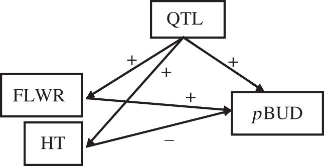
Path model of the QTL effect on pBUD. This model shows that the locus has a positive effect on the focal plant traits (HT, FLWR), and on a neighbour plant trait (pBUD). But the phenotypic effect of HT is negative, while FLWR is positive. Because FLWR has a much stronger positive effect, the overall indirect effect of the QTL on pBUD is positive.

(c). Structural equation models of interacting phenotypes

A large number of associations were found between phenotypes in the focal plants and neighbouring plants. Overall, our findings indicate that size- and development-related traits in focal plants affect size-/development-related traits in neighbouring plants. One particular focal plant latent factor (including HT, WT, FLWR, BUD, SILIQ, BRANCH, LEAF and BOLT) had effects on a neighbour plant latent factor (including pFLWR, pBUD and pBRANCH) (table 3 and figure 4). We examined the paths between the QTL and the neighbour plant latent factor, independent of the focal–neighbour phenotypic interaction; this model would encompass a portion of effects owing to the interactions that we modelled, as well as any unexplained portion owing to the locus' effects on other, unmeasured traits. This saturated model had a lower goodness of fit (χ² and Normed Fit Index; NFI) than the reduced model; so we accepted the model with only a functional pleiotropic basis indicating that the majority of the traits measured account for the interaction overall.

Table 3.

Results of structural equation model (SEM) and path analyses of the direct and indirect effects of the QTL. The focal plant traits were combined into a latent factor, and the same process was done for the neighbour plant. Two types of SEMs were constructed: an identified pleiotropy model, where the locus affected the expression of only the focal plant traits directly, and an unidentified pleiotropy model where the locus had a direct impact on (e.g. a path to) the neighbour plant traits. The effects from the identified and unidentified pleiotropy models indicate standardized regression weights (or path coefficients) indicating the relative amount of variation explained by models. Comparing the effects in the identified pleiotropy model to those in the unidentified pleiotropy model gives a measure of how much of the functional basis of the phenotypic interaction is described by the traits in the model, and in this case shows that the phenotypic ‘indentified pleiotropy model’ is a much better description of the interaction. See figure 4 for a diagram of this model.

neighbour plant traits	focal plant traits	identified pleiotropy model	unidentified pleiotropy model
pFLWR (+)	HT(−)	+0.123*	+0.056**
pBUD (+)	WT(+)
pBRANCH (+)	FLWR (+)
pLEAF (+)	BUD (+)
	SILIQ (+)
	BRANCH(+)
	LEAF(+)
	BOLT(−)

*p < 0.05.

**p < 0.01.

Figure 4.

Structural equation model (SEM) of the QTL. This SEM shows the locus mapping to a focal plant factor (size) composed of many traits. This factor impacts reproductive and structural traits in the neighbour plant. In this identified pleiotropy model, there is no path from the QTL to the neighbour's latent variable, indicating that most of the variance that is explained by this model resulted from the impact of phenotypic interactions of size on a neighbour's reproductive traits. The QTL generates an indirect genetic effect, but it is functionally mediated entirely by the locus' effects on focal plant size. Numbers represent standardized regression weights, all of which are significant (α = 0.05).

4. Discussion

Using path analysis and SEMs, we have examined the functional relationship between the genotypes and phenotypes of our focal population, and the expression of traits in their neighbours. In doing so, we examined the pleiotropic connection between direct and indirect effects (figure 1) and demonstrated that the indirect effects of a QTL of major effect on the phenotypes of neighbours are likely to be functionally mediated by the locus' direct effect on focal plant size and development, and the resulting ecological interactions with neighbours. Thus, our analysis has uncovered an explicit connection between suites of size- and development-related traits in focal plants and expression of development- and fitness-related traits in neighbouring plants. As such, this is the first study to functionally describe how a genotype–phenotype map can extend across individuals.

In order to uncover the ecological basis of IGEs, we developed two types of path models and SEMs. Our SEMs were classified as either ‘unidentified pleiotropy models’, which are those where there are connections from the focal plants' genotypes to their neighbours' phenotypes, but the connection does not appear to be mediated by the measured focal plant traits, or ‘identified pleiotropy models’, where genetic effects of the focal plants on their neighbours are mediated by phenotypic interactions involving measured focal plant traits. That is, in the identified pleiotropy models, those with a path connection between the focal plants' genotypes and their neighbours' phenotypes were better fit than models with a direct connection between QTL and partner's trait, implying that we have identified the traits closely tied to the cause (using the term loosely) of the mapping from focal genotype to neighbour phenotype (figures 1 and 2). For the SEMs, our null hypothesis was that pleiotropy would be unidentified, in that it would not be associated with the measured focal traits, and when identified pleiotropy models fit better than unidentified, we rejected that null hypothesis.

We found strong evidence for identified pleiotropy underlying the IGEs of the QTL (tables 2 and 3). The identified pleiotropy not only explained more variance in neighbour plant traits than the unidentified pleiotropy model, but it also helped to clarify and paint a more detailed picture of the nature of the indirect effects (see below). This result supports theoretical models, which propose that IGEs occur as a consequence of social interactions mediated by interacting phenotypes [22,23]. Our results also provide the first evidence towards the building of an ecological explanation for the occurrence of genetic effects that transcend individuals. We note, however, that the true form of interaction in any plant population will be reciprocal (i.e. focal plants affect their neighbours while their neighbours affect them), which can lead to feedback between trait development in the traits of interacting plants. Such reciprocal effects cannot be identified through the analyses we present here, but rather, are part of the biological process that has established the observed net effects we find statistically.

The locus on which we have focused explains a large proportion of variation in the focal plant traits (an average of 12% of the variance per trait, with a maximum of 20% in silique number; table 1). This locus was previously identified by Loudet et al. [34] in a study of flowering time and maps to a region of the genome that encompasses the FRI gene. FRI has previously been shown to have pleiotropic effects on fitness-related traits [42,43], and our analysis shows that it appears to also have relatively strong indirect effects on partners (the indirect effects alone are significant at the genome level). As expected, this QTL did have a direct effect on BOLT. It also had a direct effect on a number of size- and development-related traits (HT, WT, BRANCH, LEAF, FLWR, BUD and SILIQ). These effects may also be expected to be linked to a flowering gene, given how these traits were all measured at a fixed point in time (42 days post-germination); plants that bolted earlier were further along their development with longer inflorescence stems, more branches and flowers. While these traits should not be directly equated to total fitness, such shift in development may increase fitness if there is environmental degradation (which would cause selection to be truncated).

We found that size and fecundity-related direct traits (HT, WT, BRANCH, LEAF, FLWR, BUD and SILIQ) tied to life history in the focal individuals were the functional origin of the indirect effects of the QTL, while the traits that were affected in the partner (pFLWR, pBUD, pBRANCH, pLEAF) indicate an earlier shift to reproduction (tables 2 and 3). A possible explanation for this relationship is that when focal plants bolt earlier (as determined by the FRI locus), they significantly change the light quality in the pot for their neighbours, causing acceleration of flowering and higher internode elongation in the partner plant. Such shifts in development are commonly observed in A. thaliana and other plants in response to increased shading from its neighbours [44–47]. Since A. thaliana and other early successional weeds are poor competitors, shifting to reproduction earlier might allow escaping competition and enhance overall plant fitness [48]. This is significant because it provides a potential link between IGEs and patterns of selection, and so finding fitness-related traits involved in these sorts of functional interactions further supports IGEs' role in altering a population's evolutionary dynamics.

It is perhaps not surprising to find that ecological interactions based on size- and development-related traits occur between plants. Such ecological effects are likely to arise as a necessary consequence of nutrient acquisition, including uptake of water and nitrogen [49], suggesting that loci contributing direct genetic variation by affecting resource acquisition traits may often show up as IGEs because they affect neighbours' resource pools. Empirical work also confirms the general importance of resource-allocation patterns in intraspecific interactions [50,51]. In contrast, facilitation through microbial colonization or competition for light may lead to positive associations, as observed here. Although there are various scenarios for how loci affecting allocation patterns might have indirect effects on traits in neighbours (e.g. allocation to leaf size or height in one plant may lead to shade avoidance responses in neighbours), there is no simple general expectation for the pattern of pleiotropy of direct and indirect effects. More importantly, there could be a combination of positive and negative effects through different traits as observed in this study. The SEM built with latent factors (figure 4) shows us that the traits in the interacting plants are complex multi-dimensional phenotypes, such that the overall phenotypic interaction is a result of complicated relationships between traits within the interacting plants, even though the overwhelming pattern is of positive effect. The relationships and patterns found by examining path models and SEMs show that the analysis with identified pleiotropic effects provides a more meaningful description of relationships behind the indirect effects than does a simple QTL analysis alone. We hope that this approach will also be useful in providing a specific functional hypothesis that can then be tested experimentally.

References

- 1.Grant P. R., Grant B. R. 2006. Evolution of character displacement in Darwin's finches. Science 313, 224–226 10.1126/science.1128374 (doi:10.1126/science.1128374) [DOI] [PubMed] [Google Scholar]
- 2.Vandeleur R. K., Gill G. S. 2004. The impact of plant breeding on the grain yield and competitive ability of wheat in Australia. Aust. J. Agric. Res. 55, 855–861 10.1071/AR03136 (doi:10.1071/AR03136) [DOI] [Google Scholar]
- 3.Ackerly D. D., Schwilk D. W., Webb C. O. 2006. Niche evolution and adaptive radiation: testing the order of trait divergence. Ecology 87, S50–S61 10.1890/0012-9658(2006)87[50:NEAART]2.0.CO;2 (doi:10.1890/0012-9658(2006)87[50:NEAART]2.0.CO;2) [DOI] [PubMed] [Google Scholar]
- 4.Andalo C., Goldringer I., Godelle B. 2001. Inter- and intragenotypic competition under elevated carbon dioxide in Arabidopsis thaliana. Ecology 82, 157–164 [Google Scholar]
- 5.Astles P. A., Moore A. J., Preziosi R. F. 2005. Genetic variation in response to an indirect ecological effect. Proc. R. Soc. B 272, 2577–2581 10.1098/rspb.2005.3174 (doi:10.1098/rspb.2005.3174) [DOI] [PMC free article] [PubMed] [Google Scholar]
- 6.Cahill J. F., Kemel S. W., Gustafson D. J. 2005. Differential genetic influences on competitive effect and response in Arabidopsis thaliana. J. Ecol. 93, 958–967 10.1111/j.1365-2745.2005.01013.x (doi:10.1111/j.1365-2745.2005.01013.x) [DOI] [Google Scholar]
- 7.Griffing B. 1989. Genetic analysis of plant mixtures. Genetics 122, 943–956 [DOI] [PMC free article] [PubMed] [Google Scholar]
- 8.Mutic J. J., Wolf J. B. 2007. Indirect genetic effects from ecological interactions in Arabidopsis thaliana. Mol. Ecol. 16, 2371–2381 [DOI] [PubMed] [Google Scholar]
- 9.Johnson M. T. J., Lajeunesse M. J., Agrawal A. A. 2006. Additive and interactive effects of plant genotypic diversity on arthropod communities and plant fitness. Ecol. Lett. 9, 24–34 10.1111/j.1461-0248.2005.00833.x (doi:10.1111/j.1461-0248.2005.00833.x) [DOI] [PubMed] [Google Scholar]
- 10.Shuster S. M., Lonsdorf E., Wimp G. M., Bailey J. K., Whitham T. G. 2006. Community heritability measures the evolutionary consequences of indirect genetic effects on community structure. Evolution 60, 991–1003 10.1554/05-121.1 (doi:10.1554/05-121.1) [DOI] [PubMed] [Google Scholar]
- 11.Olofsdotter M., Jensen L. B., Courtois B. 2002. Improving crop competitive ability using allelopathy: an example from rice. Plant Breed. 121, 1–9 10.1046/j.1439-0523.2002.00662.x (doi:10.1046/j.1439-0523.2002.00662.x) [DOI] [Google Scholar]
- 12.Adamson M. L., Noble S. J. 1993. Interspecific and intraspecific competition among pinworms in the hindgut of Periplaneta americana. J. Parasitol. 79, 50–56 10.2307/3283276 (doi:10.2307/3283276) [DOI] [Google Scholar]
- 13.Peterson C. H. 1982. The importance of predation and intra- and interspecific competition in the population biology of two infaunal suspension-feeding bivalves, Protothaca staminea and Chione undatella. Ecol. Monogr. 52, 437–475 10.2307/2937354 (doi:10.2307/2937354) [DOI] [Google Scholar]
- 14.Thornhill R. 1987. The relative importance of intra- and interspecific competition in scorpionfly mating systems. Am. Nat. 130, 711–729 10.1086/284740 (doi:10.1086/284740) [DOI] [Google Scholar]
- 15.Meffert L. M. 1995. Bottleneck effects on genetic variance for courtship repertoire. Genetics 139, 365–374 [DOI] [PMC free article] [PubMed] [Google Scholar]
- 16.Petfield D., Chenoweth S. F., Rundle H., Blows M. W. 2005. Genetic variance in female condition predicts indirect genetic effects on male display traits. Proc. Natl Acad. Sci. USA 102, 6045–6050 10.1073/pnas.0409378102 (doi:10.1073/pnas.0409378102) [DOI] [PMC free article] [PubMed] [Google Scholar]
- 17.Wilson M. F. 1994. Sexual selection in plants: perspective and overview. Am. Nat. 144, S13–S39 10.1086/285651 (doi:10.1086/285651) [DOI] [Google Scholar]
- 18.Ballaré C. L., Scopel A. L., Jordan E. T., Vierstra R. D. 1994. Signaling among neighboring plants and the development of size inequalities in plant populations. Proc. Natl Acad. Sci. USA 91, 10 094–10 098 10.1073/pnas.91.21.10094 (doi:10.1073/pnas.91.21.10094) [DOI] [PMC free article] [PubMed] [Google Scholar]
- 19.Nilsson C. 1994. Separation of allelopathy and resource competition by the boreal dwarf shrub Empetrum hermaphroditum Hagerup. Oecologia 98, 1–7 10.1007/BF00326083 (doi:10.1007/BF00326083) [DOI] [PubMed] [Google Scholar]
- 20.Ridenour W. M., Callaway R. M. 2001. The relative importance of allelopathy in interference: the effects of an invasive weed on a native bunchgrass. Oecologia 126, 444–450 10.1007/s004420000533 (doi:10.1007/s004420000533) [DOI] [PubMed] [Google Scholar]
- 21.Griffing B. 1967. Selection in reference to biological groups. I. Individual and group selection applied to populations of unordered groups. Aust. J. Biol. Sci. 20, 127–139 [PubMed] [Google Scholar]
- 22.Wolf J. B., Moore A. J. 2010. Interacting phenotypes and indirect genetic effects: a genetic perspective on the evolution of social behavior. In Evolutionary behavioral ecology (eds Westneat D. F., Fox C. W.). New York, NY: Oxford University Press [Google Scholar]
- 23.Moore A. J., Brodie E. D., III, Wolf J. B. 1997. Interacting phenotypes and the evolutionary process. I. Direct and indirect genetic effects of social interactions. Evolution 51, 1352–1362 10.2307/2411187 (doi:10.2307/2411187) [DOI] [PubMed] [Google Scholar]
- 24.Wolf J. B., Brodie E. D., III, Cheverud J. M., Moore A. J., Wade M. J. 1998. Evolutionary consequences of indirect genetic effects. Trends Ecol. Evol. 13, 64–69 10.1016/S0169-5347(97)01233-0 (doi:10.1016/S0169-5347(97)01233-0) [DOI] [PubMed] [Google Scholar]
- 25.Goldberg D. E., Landa K. 1991. Competitive effect and response: hierarchies and correlated traits in the early stages of competition. J. Ecol. 79, 1013–1030 10.2307/2261095 (doi:10.2307/2261095) [DOI] [Google Scholar]
- 26.Mitchell R. J. 1992. Testing evolutionary and ecological hypotheses using path analysis and structural equation modelling. Funct. Ecol. 6, 123–129 10.2307/2389745 (doi:10.2307/2389745) [DOI] [Google Scholar]
- 27.Wootton J. T. 1994. Predicting direct and indirect effects: an integrated approach using experiments and path analysis. Ecology 75, 151–165 10.2307/1939391 (doi:10.2307/1939391) [DOI] [Google Scholar]
- 28.Crespi B. J. 1990. Measuring the effect of natural selection on phenotypic interaction systems. Am. Nat. 135, 32–47 10.1086/285030 (doi:10.1086/285030) [DOI] [Google Scholar]
- 29.Crespi B. J., Bookstein F. L. 1989. A path-analytic model for the measurement of selection on morphology. Evolution 43, 18–28 10.2307/2409161 (doi:10.2307/2409161) [DOI] [PubMed] [Google Scholar]
- 30.Geber M. A., Griffen L. R. 2003. Inheritance and natural selection on functional traits. Int. J. Plant Sci. 164, S21–S42 10.1086/368233 (doi:10.1086/368233) [DOI] [Google Scholar]
- 31.Eaves L. J., Neale M. C., Maes H. 1996. Multivariate multipoint linkage analysis of quantitative trait loci. Behav. Genet. 26, 519–525 10.1007/BF02359757 (doi:10.1007/BF02359757) [DOI] [PubMed] [Google Scholar]
- 32.Stein C. M., Song Y., Elston R. C., Jun G., Tiwari H. K., Iyengar S. K. 2003. Structural equation model-based genome scan for the metabolic syndrome. BMC Genet. 4, S99. 10.1186/1471-2156-4-S1-S99 (doi:10.1186/1471-2156-4-S1-S99) [DOI] [PMC free article] [PubMed] [Google Scholar]
- 33.Li R., Tsaih S.-W., Shockley K., Stylianou I. M., Wergedal J., Paigen B., Churchill G. A. 2006. Structural model analysis of multiple quantitative traits. PLoS Genet. 2, e114. 10.1371/journal.pgen.0020114 (doi:10.1371/journal.pgen.0020114) [DOI] [PMC free article] [PubMed] [Google Scholar]
- 34.Loudet O., Chaillou S., Camilleri C., Bouchez D., Daniel-Vedele F. 2002. Bay-0 × Shahdara recombinant inbred line population: a powerful tool for the genetic dissection of complex traits in Arabidopsis. Theor. Appl. Genet. 104, 1173–1184 10.1007/s00122-001-0825-9 (doi:10.1007/s00122-001-0825-9) [DOI] [PubMed] [Google Scholar]
- 35.Leamy L. J., Routman E. J., Cheverud J. M. 1999. Quantitative trait loci for early- and late-developing skull characters in mice: a test of the genetic independence model of morphological integration. Am. Nat. 153, 201–214 10.1086/303165 (doi:10.1086/303165) [DOI] [PubMed] [Google Scholar]
- 36.Wolf J. B., Leamy L., Routman E. J., Cheverud J. M. 2005. Epistatic pleiotropy and the genetic architecture of covariation within early- and late- developing skull trait complexes in mice. Genetics 171, 683–694 10.1534/genetics.104.038885 (doi:10.1534/genetics.104.038885) [DOI] [PMC free article] [PubMed] [Google Scholar]
- 37.Bollen K. 1989. Structural equations with latent variables. Wiley Series in Probability and Mathematical Statistics Chichester, UK: John Wiley & Sons [Google Scholar]
- 38.Loehlin J. 1992. Latent variable models: an introduction to factor, path and structural analysis, 2nd edn London, UK: Lawrence Erlbaum Associates [Google Scholar]
- 39.Bozdogan H. 1987. Model selection and Akaike's information criterion (AIC): the general theory and its analytical extensions. Psychometrika 52, 345–370 10.1007/BF02294361 (doi:10.1007/BF02294361) [DOI] [Google Scholar]
- 40.Roux F., Touzet P., Cuguen J., Le Corre V. 2006. How to be early flowering: an evolutionary perspective. Trends Plant Sci. 11, 375–381 10.1016/j.tplants.2006.06.006 (doi:10.1016/j.tplants.2006.06.006) [DOI] [PubMed] [Google Scholar]
- 41.Korves T. M., Schmid K. J., Caicedo A. L., Mays C., Stinchcombe J. R., Purugganan M. D., Schmitt J. 2007. Fitness effects associated with the major flowering time gene FRIGIDA in Arabidopsis thaliana in the field. Am. Nat. 169, E141–E157 10.1086/513111 (doi:10.1086/513111) [DOI] [PubMed] [Google Scholar]
- 42.Mckay J. K., Richards J. H., Mitchell-Olds T. 2003. Genetics of drought adaptation in Arabidopsis thaliana. I. Pleiotropy contributes to genetic correlations among ecological traits. Mol. Ecol. 12, 1137–1151 10.1046/j.1365-294X.2003.01833.x (doi:10.1046/j.1365-294X.2003.01833.x) [DOI] [PubMed] [Google Scholar]
- 43.Scarcelli N., Cheverud J. M., Schaal B., Kover P. X. 2007. Antagonistic pleiotropy reduce the potential adaptive value of the FRIGIDA locus. Proc. Natl Acad. Sci. USA 104, 16 986–16 991 10.1073/pnas.0708209104 (doi:10.1073/pnas.0708209104) [DOI] [PMC free article] [PubMed] [Google Scholar]
- 44.Devlin P. F., Robson P. R., Patel S. R., Sharrock R. A., Whitelam G. C. 1999. Phytochrome D acts in the shade-avoidance syndrome in Arabidopsis by controlling elongation growth and flowering time. Plant Physiol. 119, 909–916 10.1104/pp.119.3.909 (doi:10.1104/pp.119.3.909) [DOI] [PMC free article] [PubMed] [Google Scholar]
- 45.Halliday K. J., Koornneef M., Whitelam G. C. 1994. Phytochrome B and at least one other phytochrome mediate the accelerated flowering response of Arabidopsis thaliana L. to low red/far-red ratio. Plant Physiol. 104, 1311–1315 [DOI] [PMC free article] [PubMed] [Google Scholar]
- 46.Ballaré C. L., Scopel A. L., Jordan E. T., Vierstra R. D. 1994. Signaling among neighboring plants and the development of size inequalities in plant populations. Proc. Natl Acad. Sci. USA 91, 10 094–10 098 10.1073/pnas.91.21.10094 (doi:10.1073/pnas.91.21.10094) [DOI] [PMC free article] [PubMed] [Google Scholar]
- 47.Martínez-García J. F., Galstyan A., Salla-Martret M., Cifuentes-Esquivel N., Gallemí M., Bou-Torrent J. 2010. Regulatory components of shade avoidance syndrome. Adv. Bot. Res. 53, 65–116 10.1016/s0065-2296(10)53003-9 (doi:10.1016/s0065-2296(10)53003-9) [DOI] [Google Scholar]
- 48.Callahan H. S., Pigliucci M. 2002. Shade-induced plasticity and its ecological significance in wild populations of Arabidopsis thaliana. Ecology 83, 1965–1980 [Google Scholar]
- 49.DeFalco L. A., Bryla D. R., Smith-Longozo V., Nowak R. S. 2003. Are Mojave Desert annual species equal? Resource acquisition and allocation for the invasive grass Bromus madritensis subsp. rubens (Poaceae) and two native species. Am. J. Bot. 90, 1045–1053 10.3732/ajb.90.7.1045 (doi:10.3732/ajb.90.7.1045) [DOI] [PubMed] [Google Scholar]
- 50.Lynch J. P., Ho M. D. 2005. Rhizoeconomics: carbon costs of phosphorus acquisition. Plant Soil 269, 45–56 10.1007/s11104-004-1096-4 (doi:10.1007/s11104-004-1096-4) [DOI] [Google Scholar]
- 51.Reich P. B., Wright I. J., Cavender-Bares J., Craine J. M., Oleksyn J., Westoby M., Walters M. B. 2003. The evolution of plant functional variation: traits, spectra, and strategies. Int. J. Plant Sci. 164, 143–164 10.1086/374368 (doi:10.1086/374368) [DOI] [Google Scholar]