

Abstract
A central question in community ecology is how the number of trophic links relates to community species richness. For simple dynamical food-web models, link density (the ratio of links to species) is bounded from above as the number of species increases; but empirical data suggest that it increases without bounds. We found a new empirical upper bound on link density in large marine communities with emphasis on fish and squid, using novel methods that avoid known sources of bias in traditional approaches. Bounds are expressed in terms of the diet-partitioning function (DPF): the average number of resources contributing more than a fraction f to a consumer's diet, as a function of f. All observed DPF follow a functional form closely related to a power law, with power-law exponents independent of species richness at the measurement accuracy. Results imply universal upper bounds on link density across the oceans. However, the inherently scale-free nature of power-law diet partitioning suggests that the DPF itself is a better defined characterization of network structure than link density.
Keywords: community structure, stability, complexity–diversity, interaction strength, species richness, food webs
1. Introduction
Relationships between biodiversity and the stability and complexity of ecological communities are central to understanding their assembly, structure, function and persistence, and hence important for conservation. Odum [1], MacArthur [2] and others initiated the so-called complexity–diversity–stability debate nearly 60 years ago. By now, we learned that the answers to the questions asked then critically depend on their precise formulation [3]. Here we address one specific set of questions—originally posed by MacArthur [2,4] and May [5] and still being discussed today [6–8]—concerning the relation between the number of species S and the number of trophic links L (i.e. consumer–resource pairs) in large natural food webs. Because link counts L inevitably increase with community size, they are ‘normalized’ (descaled) by dividing by the potential number of links, giving the connectance or ‘complexity’ C = L/S2, or by species richness, giving the link density Z = L/S of the community (see table 1 for a list of symbols).
Table 1.
List of important symbols.
| symbol | meaning |
|---|---|
| α, γ | exponents for scaling with S |
| ν | exponent for scaling of Zc with r |
| νi | ν measured in system i |
| ν̄ | sample mean of ν |
| Δνi | residuals of regression of ν against log-effort |
| C | food-web connectance |
| E | total number of non-empty stomachs sampled |
| ei | standard error of νi |
| fij | diet fraction: relative contribution of i to j's diet |
| f | diet-fraction threshold |
| L | number of trophic links in a food web |
| r | diet-ratio threshold = f/(1 − f) |
| S | species richness |
| Sc | consumer species richness |
| Sp | producer species richness |
| Sfish | fish species richness |
| sν | sample standard deviation of ν |
| Z | links per species |
| Zc | links per consumer |
| Zc(f) | diet-partitioning function (DPF) |
Mathematical arguments and simulations by Gardner & Ashby [4], May [5] and others (using simple models of large random communities) showed that there are upper limits to link density, Z = CS, beyond which community steady states become unstable, ultimately leading to species extinctions [9]. Communities with numerically large Z should therefore not be observable in the field. Early empirical studies appeared to confirm this prediction (e.g. [10,11], but later work using larger food-web datasets contradicted the theoretical expectations (e.g. [8,12–15]). In these studies, scaling laws such as Z ∝ Sα were found, with values of α ranging from 0.3 [15] to 1 [14], conforming with the long-standing empirical intuition that ‘complexity begets stability’. These observations motivated an intense search for mechanisms that could stabilize communities with large S and Z (e.g. [16–25]).
However, there are a number of issues that, although known and acknowledged in principle [7,26–31], have not been fully and jointly accounted for in the analyses of food-web data.
Three facts in particular are important: most trophic links are weak [32,33] empirical food-web datasets vary in their resolution of taxonomic or functional groups [27,28], and criteria for recording or excluding particular trophic links vary between datasets [30]. Without giving these three issues sufficient consideration, conclusions drawn from analyses of food-web topologies regarding complexity–diversity and complexity–stability relations might be premature.
To overcome these problems, we use here the diet-partitioning function (DPF), proposed by Rossberg et al. together with a protocol for calculating it from incompletely resolved diet data [34]. We express link strengths in terms of gravimetric or volumetric diet fractions, i.e. proportional contributions to a consumer's diet—a common theoretical [35] and empirical [30,31] convention—such that fij is the fraction of the total diet of species j that is made up of species i. The DPF Zc(f) is defined as the community average of the number of prey species that contribute more than a fraction f to the diet of a consumer species, where f takes values between 0 and 1. The value of Zc(f) can be interpreted as the mean number of trophic links per consumer, where only those links that are stronger than f are counted.
If Sc is the number of consumer species and Sp is the number of producer (autotrophic) species in a community (so that Sc + Sp = S) then, irrespective of the criterion for counting links, the consumer link density Zc = L/Sc must always be larger than the link density Z = L/(Sc + Sp), because Sp > 0. Since Zc equals the mean number of prey per consumer, it can be estimated from a sub-sample of consumer species. It is therefore measured more easily than Z for large communities.
In this paper, we use Zc to test whether there is an upper bound to Z; specifically, we test if Zc increases with species richness S because, if it does not, then Zc > Z implies that Z must be bounded from above for increasing S. Conversely, an unbounded increase of Z with S implies an unbounded increase of Zc with S. Counting only links stronger than f, but keeping f variable, we report estimates of Zc = Zc(f) in relation to S, taken from seven different marine stomach-contents datasets. Based on our analysis, we will argue that the DPF Zc(f) itself might be a more suitable characterization of communities than any particular value Zc extracted from it.
2. Material and methods
(a). Calculation of DPF
We use the diet ratio rij = fij/(1 − fij), comparing the contribution of the ith diet item to the sum of all other contributions to the diet of j, as an alternative measure to the diet fraction fij. Diet ratios can attain values in the range [0;∞] and, like ‘odds’ in statistics, are the natural choice on logarithmic scales.
The basic idea underlying the correction of the DPF for unresolved diet items is to first count only those diet items that are resolved to species level, and then to compensate for the proportion of diets left out. A detailed illustration of the method and hands-on instructions for its implementation are given in electronic supplementary material, appendix S1. For a systematic derivation, see Rossberg et al. [34].
(b). Diet data
The DPF Zc(f) was computed for seven stomach-contents datasets (labelled A–G) of marine fish and squid [36–40]. As illustrated in figure 1, sample sites span a broad latitudinal range. Key properties of the datasets are listed in table 2. Data sources differ considerably by sampling methods, sampling efforts and the kinds of species included. Details are discussed in electronic supplementary material, appendix S2.
Figure 1.

Approximate locations of sampling sites.
Table 2.
Datasets included in the analysis.
| dataset | Sfish AquaMaps | Sfish FishBase + OBIS | consumer species included | resource species resolved | non-empty stomachs |
|---|---|---|---|---|---|
| (A) N.-W. Atlantic Shelf I | 247 | 645 | 146 | 767 | 29 032 |
| (B) N.-W. Atlantic Shelf II | 247 | 645 | 117 | 216 | 50 027 |
| (C) Open North Atlantic | 335 | 679 | 17 | 19 | 188 |
| (D) Open Tropical Atlantic | 340 | 179 | 18 | 24 | 357 |
| (E) North Sea | 103 | 192 | 15 | 91 | 5599 |
| (F) South China Sea | 512 | 3827 | 18 | 14 | ∼1007 |
| (G) Eastern Bering Sea | 92 | 250 | 25 | 137 | 17 688 |
(c). Fitting curves to observed DPF
Characterizations of the DPF in terms of theoretical or heuristic models should be based only on a range of diet fractions f for which the data are reliable. For obvious practical reasons, actual or conceivable diet items making very small (rare) contributions to a consumer's diet are unlikely to be observed and recorded, leading to an underestimation of the DPF for low threshold values. As f increases, the probability of observation gradually increases, up to a point above which sampling is essentially complete and empirical DPF, while still exhibiting measurement errors, are unbiased. Based on the number of non-empty stomachs sampled per consumer, we assume this point to be somewhere below f = 0.02, i.e. that sampling of contributions larger than f = 0.02 is essentially complete (see also electronic supplementary material, supplementary discussion S6). In terms of diet ratios, this corresponds to the range 0.02≲r ≲ 50, which we shall call the reliable range.
Models for the DPF, such as equation (3.2) below, were fitted to the data over this reliable range by a likelihood maximization technique. Details of the procedure are described in electronic supplementary material, appendix S3.
(d). Species richness
Traditionally, diversity–complexity studies measure diversity by the numbers of nodes distinguished in empirical food-web datasets. Since here only sub-samples of food webs are used, information on species richness has to be obtained independently. Fortunately, only relative richness estimates are required for our argument. Further, as shown in a detailed, quantitative discussion of these questions in electronic supplementary material, supplementary discussion S6.2, rather coarse richness estimates are sufficient to support our main conclusion.
We use estimates of species richness based on the FishBase [41], OBIS [42] and AquaMaps [43]. These databases have global coverage, and therefore allow us to obtain, with a few exceptions, richness estimates specific to the study sites considered here. All three databases are substantially more detailed for fish than for most other taxa. To reduce biases owing to data gaps, relative richness is therefore measured in terms of richness of fish, Sfish, including Actinopterygii, Chondrichthyes and Agnatha for FishBase and OBIS, and only Actinopterygii (the dominating taxon) for AquaMaps. Overall, marine species richness is known to follow the same global trends as that of fish, with some variation in details [44]. This fact and the low demands on accuracy mentioned above justify our choice of Sfish as an estimate of relative richness. This measure has the additional advantage that its empirical uncertainty has been quantified [45], allowing a quantification of the uncertainty this implies for our main results. As shown in electronic supplementary material, supplementary discussion S6.2, this uncertainty is small when compared with that stemming from the dietary analysis.
Despite this robustness to uncertainties in richness estimates, we performed our analysis using two sets of values for Sfish, one derived from AquaMaps, the other from FishBase and OBIS. The reason is that both approaches have specific strengths: FishBase + OBIS data are based on direct observations and therefore methodologically more transparent; AquaMaps is more robust to data gaps, and richness estimates specific to the delineations of the study areas A–G can be obtained (see electronic supplementary material, appendix S4 for details). Estimated species richnesses Sfish are listed in table 2. The much lower FishBase + OBIS richness in the Tropical Atlantic (set D) when compared with the North Atlantic is inconsistent with other estimates [44] and most likely attributable to data gaps [42].
Because the FishBase richness estimate for fish in the ‘South China Sea’ (3827) is considerably larger than our estimate for study area F using AquaMaps (512, the most species-rich study area), the nominal accuracy of the estimated slope of link density versus diversity turns out to be substantially higher when using the FishBase + OBIS data. To caution against inflated accuracy, we therefore conservatively report detailed results using the AquaMaps richness measures below, followed by short summaries of the corresponding results using FishBase + OBIS.
3. Results
(a). Computation and characterization of empirical DPF
The DPF estimated from sets A–G are shown in figure 2, with the threshold f expressed as a diet ratio, r = f/(1 − f). Surprisingly, all DPF except for set C (blue) match a single curve, suggesting the possibility of a universal law for diet partitioning within these communities. Over the reliable range in r (see §2c), 0.02 ≲ r≲50, the curves appear to follow power laws (straight lines in log–log graphs), mirroring a recent similar observation of power law [46] rather than exponentially distributed [32,33] trophic fluxes.
Figure 2.

Comparison of seven empirical DPF from six marine areas. The diet ratio r is the contribution of one prey species to a consumer's diet relative to all other contributions. Solid lines: datasets A–G. Dashed line: power-law equation (3.2) with ν = 0.54. Red, A; green, B; blue, C; violet, D; pink, E; orange, F; light blue, G.
This allows us to describe the DPF in the power-law form: Zc = Kr−ν. The constant of proportionality K can now be computed from the condition
| 3.1 |
which follows from the fact that all diet fractions of a consumer add up to one [34]. One obtains K = π−1ν−1 sin(πν) for 0 < ν < 1, giving
| 3.2 |
Beyond the reliable range, when r ≲ 0.02, the empirical DPF in figure 2 decline in slope to near zero, clearly deviating from power laws. This may result from incomplete sampling of small diet fractions, but may conceivably show a true underlying deviation from power laws at very low diet-ratio thresholds. We consider resolving these possibilities in electronic supplementary material, supplementary discussion S6, and here restrict our analysis to the reliable range (0.02 ≲ r≲50), addressing the following three questions: (i) are the empirical DPF consistent with power laws over the reliable range in r? (ii) What values of the exponent  best fit the empirical DPF over the reliable range? (iii) How do the fitted values vary among study sites?
Estimates of ν from maximum-likelihood fits of the power law (3.2) to the empirical DPF over the reliable range and related statistics are listed in table 3 (details provided in electronic supplementary material, appendix S3). Goodness-of-fit by χ2-statistics shows that all empirical DPF are compatible with power laws (table 3). For comparison, models with exponential and logarithmic dependencies of Zc on r score considerably worse by χ2-statistic and by the Akaike Information Criterion (AIC, see table 3 and also electronic supplementary material, appendix S3).
Table 3.
Results of maximum-likehood fits of three functional forms to the observed DPF.
| assumed functional forma: |
Zc ∝ r−ν |
Zc ∝ max[ln(c2/r),0] |
Zc ∝ exp(−c1r) |
|||||||
|---|---|---|---|---|---|---|---|---|---|---|
| dataset | ν ± s.e.m. | d.o.f. | χ2 | p | χ2 | p | ΔAICb | χ2 | p | ΔAICb |
| (A) N.-W. Atlantic Shelf I | 0.53 ± 0.03 | 56 | 35.3 | 0.99 | 506.9 | <10−9 | 998.2 | 415.3 | <10−9 | 338.1 |
| (B) N.-W. Atlantic Shelf II | 0.56 ± 0.04 | 44 | 33.2 | 0.88 | 224.5 | <10−9 | 393.4 | 223.0 | <10−9 | 165.4 |
| (C) Open North Atlantic | 0.30 ± 0.09 | 10 | 13.5 | 0.20 | 79.3 | <10−9 | 98.5 | 26.3 | 0.003 | 9.4 |
| (D) Open Tropical Atlantic | 0.55 ± 0.11 | 19 | 10.7 | 0.93 | 38.3 | 0.005 | 34.5 | 30.8 | 0.04 | 8.1 |
| (E) North Sea | 0.50 ± 0.10 | 20 | 10.2 | 0.96 | 47.2 | 0.001 | 47.7 | 26.2 | 0.16 | 6.3 |
| (F) South Chinese Sea | 0.43 ± 0.12 | 13 | 11.3 | 0.58 | 52.6 | 10−6 | 51.4 | 25.2 | 0.02 | 7.1 |
| (G) Eastern Bering Sea | 0.58 ± 0.07 | 22 | 25.3 | 0.28 | 111.2 | <10−9 | 145.3 | 63.9 | 10−5 | 25.5 |
aν, c1, c2 are fitting parameters; proportionality constants are given by equation (3.1).
bExcess AIC relative to power-law fits; positive values indicate that power law is the preferred model.
Thus, over the reliable range, all DPF Zc(f) statistically match power laws that are wholly characterized by the exponent ν. For power-law DPF, constancy of ν over a range of species richness Sfish implies constancy of consumer link density Zc(f) at varying species richness for any value of the diet-fraction threshold f. Comparisons of link densities across study areas are therefore most efficiently carried out as comparisons of the fitted exponents ν across study areas.
(b). Comparison of the power-law exponent ν across study sites
The maximum-likelihood fitting procedure for the power-law equation (3.2) yields Cramér-Rao lower bounds as estimates for the standard errors ei of the fitted parameter ν (table 3) for each dataset i. This information (not entering conventional regression analysis) was used to estimate the accuracy of fitted regression models. Specifically, 106 Monte Carlo simulations of the null model
| 3.3 |
with standard-normal ξi were generated. Species richnesses and sampling efforts were fixed as in table 2, and, without loss of generality, we set ν* = 0. By evaluating the simulated data just as the measured data, standard errors of regression coefficients and p-values for null hypotheses were obtained. Confidence intervals were computed by offsetting the corresponding distributions of the simulated data by the estimated values obtained from the measured data (which is admitted by the linearity of the regression models and the symmetry of standard normal distributions).
(i). Cross-site comparison of exponents without correction for effort
Assuming that the power-law exponents for all study systems share a common value, the maximum-likelihood estimate ν̄ for this value can be computed as the weighted average of the values listed in table 2, with the weights chosen as the inverse variances of the estimation errors 1/ei2. In what follows, all means and regressions are computed with this weighting of datasets. We obtain ν̄ = 0.54(2) (digits in parenthesis represent standard errors estimated using model (3.3)).
To test the null hypothesis that all exponents are equal, we computed the statistic SS0 = ∑i(νi − ν̄)2ei−2 = 8.4. Comparison with model (3.3) shows that data are consistent with this hypothesis at p = 0.21, that is, SS0 computed using simulated data from model (3.3) is larger than the empirical value in 21 per cent of all cases.
The weighted sample standard deviation of ν is sν = 0.032, giving a coefficient of variation CV = sν/ν̄ = 0.06. By an argument detailed in electronic supplementary material, supplementary discussion S6.2, this small CV itself strongly constrains the scope for any systematic variation of ν with species richness, independent of the particular measure of species richness used.
However, specific tests for the dependence of ν on species richness have stronger statistical power than, e.g. the simple test for equal means above. For example, a regression of ν against AquaMaps estimates of species richness Sfish yields ν = 0.62(7) − 0.00040(27) Sfish. The 95 per cent confidence region for this regression, together with measured ν values, is shown in figure 3a. Despite the weak negative trend, the regression coefficient is consistent with the null hypothesis that ν is independent of Sfish at p = 0.14.
Figure 3.

Dependencies of diet-partitioning exponent ν on species richness and sampling effort. Each point represents one dataset. In (c) ν is corrected for effort. Error bars indicate s.e. Dotted lines are regressions of ν against (a) species richness, (b) inverse effort and (c) both. Shaded areas in panels (a) and (c) indicate 95% confidence regions of regression lines.
Using the FishBase + OBIS richness estimates, the slope of the regression of ν on Sfish becomes −0.000034(36), consistent with zero at p = 0.35. Inclusion or exclusion of dataset D in this analysis (for its questionable richness estimate) gives numerically identical results.
(ii). Cross-site comparison of exponents with correction for effort
Figure 3b shows empirical values of ν drawn against sampling effort E, measured in terms of the number of non-empty stomachs analysed. The graph indicates a weak dependence of ν on effort. To check this hypothesis we compared the AIC for model fits of the forms ν = a (ΔAIC = 0), ν = a + bE (ΔAIC = −0.98), ν = a + bE−1 (ΔAIC = −3.95) and ν = a + b log E (ΔAIC = −3.01). While not unequivocal, the negative ΔAIC for the last three models suggest that values of ν are somewhat biased by sampling effort. A bias proportional to E−1 (third model) is favoured by the AIC and appears plausible because asymptotic low-sample-size biases of this form are often encountered in statistics. The dotted line in figure 3b is the corresponding fitted curve. It is given by ν = 0.54(2) − 40(16)E−1, with the second term describing a bias at low sampling efforts. Exponents ν corrected for this bias are shown in figure 3c.
Indeed, while numerically leaving the overall estimate ν̄ = 0.54(2) unchanged, the correction for effort improves the consistency of measured diet-partitioning exponents ν across study sites. Based on the statistic SS = ∑i (Δνi)2 ei−2 = 2.4, where Δνi are the residuals of the regression against E−1, the null hypothesis of equal ν across study sites after correction is consistent with the data with p = 0.78 (by comparison of SS with simulations of model (3.3), including simulated corrections for effort).
Correction for effort also removes the weak negative dependence of diet breadth on species richness. A combined regression of ν against sampling effort and species richness (AquaMaps) yields ν = 0.57(7) − 36(18)E−1 − 0.00014(30)Sfish. The 95 per cent confidence region of this regression for infinite effort is indicated in figure 3c. Since we simultaneously regressed against effort and species richness, this confidence region accounts for uncertainties by both the correction for effort and the regression on Sfish. (Strong correlations between E−1 and Sfish would broaden this region rather than narrowing it.) Comparing the regression slope with simulations of model (3.3), the null hypothesis that corrected ν do not depend on Sfish is fully supported (p = 0.65). A statistic characterizing the strength of the dependence of one empirical quantity on another (rather than the strength of evidence for a dependence) is the elasticity at the sample means ([47], see also electronic supplementary material, appendix S6.2), obtained by normalizing the regression slope to the sample means of the two variables. With weighted mean species richness S̄fish = 243.1, the elasticity of the dependence of ν on Sfish evaluates to −0.06(14). When assuming a power-law relation between ν and Sfish, we obtain ν = 0.67(Sfish)−0.04 with a 95% confidence interval (−0.12, 0.25) for the exponent, again after correcting for insufficient sampling (and using an adaptation of model (3.3) to handle this case).
When using FishBase + OBIS richness estimates, the p-value for independence of ν from Sfish becomes 0.42 when including set D and 0.55 when excluding it. The regression slope for the dependence of corrected ν on Sfish becomes −0.000029(36) (elasticity −0.036(45)) when including and −0.000022(37) (elasticity −0.028(47)) when excluding set D.
All results reported above are consistent with constant ν, and therefore constant consumer link density across study systems, and the data impose tight bounds on any conceivable dependence of link-density on species richness.
4. Discussion
(a). Diversity–complexity implications
We found that, to the accuracy of our analysis, all DPF followed a power law over the reliable range, which covers more than three orders of magnitude in diet ratios, and that the power-law exponent ν is independent of species richness Sfish. We cannot exclude a weak positive or negative dependence of ν on species richness, but a steady decline of ν to zero as Sfish goes to zero seems unlikely in view of the low upper bound for the exponent of a conceived power-law relation ν ∝ Sfishγ (−0.25 ≤γ ≤ 0.12).
If the DPF exponent ν is independent of local species richness, then so is consumer link density Zc(f) at any fixed threshold f within the reliable range. This, in turn, implies an upper bound on the conventional link density Z (with links thresholded at f) that is independent of community size. This means that Z could, for example, approach some constant, or may steadily decrease as species richness increases. Even if the DPF slightly deviated from a perfect power law, this would lead only to small additional uncertainties and not affect the role of Zc(f) as an upper bound on Z. Observations and theory suggest that consumers have broader diets at higher trophic levels [23,48], so the inevitable over-sampling of consumers from higher trophic levels will rather over- than underestimate Zc, reinforcing the interpretation of Zc as an upper bound for Z.
Despite these clear findings, it is not a simple matter to draw definite conclusions in terms of link density Z or consumer link density Zc, as that would raise questions such as how link strength is best measured, how the threshold f is best chosen, if it might need to be adjusted with system size, or if simply all links have to be counted (f = 0). Such questions (addressed in depth in electronic supplementary material, supplementary discussion S6.3) relate much more to what, by definition, should count as a ‘trophic link’ than to actual ecological phenomena. The power-law nature of the DPF reinforces these questions, because power laws are, in contrast to other kinds of functional relationships, ‘scale free’ [49]. This means that a characteristic scale of the independent variable (here r) is not implied in the functional relationship itself.
To sidestep the question how trophic links are to be counted (or weighted, see [8]), we wish to suggest reformulating the basic problem addressed here as a problem concerning relations between the distribution of trophic link strengths and local species richness (both, by specific measures). Specifically, we asked here if the DPF changes as species richness changes across the oceans. The answer we found was that, for fish and squid, stomach-contents data showed no significant changes, so implying a universal form: that of the power law, equation (3.2) (at least in the range of diet ratios 0.02 ≲ r≲50). These findings were anticipated by figure 2, and the subsequent statistical analyses fully confirmed them.
In electronic supplementary material, supplementary discussion S6.1, we detail a possible explanation for the universal power law; essentially that it arises from zooming into the upper tail of a diet-ratio distribution that is broad on a logarithmic scale (see [49] for a general discussion of power laws and mechanisms). But this explanation does not clarify why the exponent ν attains a universal value. Further study will be needed to understand the underlying mechanisms. This may be achieved by adapting theories that invoke the presence or absence of trophic-link to situations with broad distributions of link strengths on logarithmic scales. Good starting points might be theories examining limits to link density through limits to the stability [5], invadibility [50] or feasibility [51] of communities, and limits on the occurrence of—potentially destabilizing [52]—loops in interaction networks [53]. Generalizations of such theories will express the respective limits in terms of the DPF or similar characterizations of link-strength distributions.
Our characterization of the DPF is currently valid down to diet fractions of 0.02 and it is not yet clear whether this resolution is sufficient to distinguish between different theories for mechanisms controlling link density, or to judge what the implications of the observed DPF are for ecosystem properties such as stability, invadibility or feasibility. Only with the more general theories at hand will we be able to answer these questions. As an illustration, let us speculate that the diet fractions fij of a consumer j enter a relevant theoretical formula, e.g. through
 |
4.1 |
a quantity closely related to Lloyd's [54] ‘mean crowding’ [55]. ‘Niche breadth’ sensu Levins [56] is simply the inverse  [55]. Invoking the probabilistic interpretation of the DPF [34], the expectation value of
  is computed in electronic supplementary material, appendix S5 as
| 4.2 |
(where Z′c(f) = dZc(f)/df). For power-law DPF following equation (3.2) with 0 < ν < 1, this integral evaluates to  . With the exponent ν = 0.54 previously found,
  . How much uncertainty does our inability to resolve the DPF for f < 0.02 add to this result? Consider the extreme and obviously counterfactual (figure 2) case that no diet fractions <0.02 exist at all. The corresponding DPF is constant for f ≤ 0.02, and requires a correction of normalization according to equation (3.1). With this DPF, formula (4.2) evaluates to
  . The resulting uncertainty in
  is 0.06 (plus the measurement uncertainty in ν of similar magnitude). This might be sufficiently small to distinguish between different theoretical models and predictions for dietary diversity in the oceans. We caution, however, that the DPF could enter theory through expressions very different from equation (4.2), perhaps giving more weight to small diet fractions.
(b). Separation of contributions to empirical DPF
The DPF and the diet-partitioning exponent ν are highly integrated summary statistics. To inform and constrain theories aimed at explaining their observed constancy, a separation of distinct contributions to these statistics can be helpful. This shall here be illustrated by two contrasting examples.
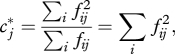
Define the consumer-specific DPF for a given consumer species as the number of this consumer's diet fractions larger than a threshold value f. The (proper) DPF Zc(f) is the arithmetic mean of all consumer-specific DPF over a community. Figure 4 displays approximations of the consumer-specific DPF of all consumers who contribute to dataset A. Immediately apparent is the large variability among consumers. To characterize this variability, we fixed the threshold diet ratio at r = f/(1 − f) = 0.02 (dashed line), and computed the cumulative distribution of the number of diet fractions greater than f, that is, of thresholded consumer generality [12]. The distribution is shown in the inset of figure 4. Following Camacho et al. [57], we normalized generality to its mean (=Zc(f)). This allows a direct comparison with a heuristic generality distribution function that was shown by Camacho et al. [57] to describe binary food-web data well (dash-dotted line). Both distributions are characterized by a wide spread and a strong skew towards small generality. Apparently, the large variability of consumer-specific DPF reflects a corresponding phenomenon for binary food webs, presumably resulting from phylogenetic clustering [58–60]. The large variability among consumer-specific DPF, not found among community DPF, suggests that the mechanism regulating the diet-partitioning exponent ν operates rather at the community level than at species or individual level.
Figure 4.

Consumer-specific DPF for dataset A (main panel) and distribution of generality (inset) for diet contributions larger than r = 0.02 (dashed vertical line). The dash-dotted line corresponds to the generality distribution proposed by Camacho et al. [57,62].
As a second example, figure 5 displays a time series of yearly diet-partitioning exponents (±s.e.) computed from datasets A and B. Each year over 1500 non-empty stomachs were sampled, so that, by figure 3b, biases owing to insufficient sampling are not expected. Even though overall deviations of the yearly slopes from the sample mean are larger than expected from the computed standard errors (χ2-test, p = 0.01), these deviations are too small to be associated with any particular structure in the data. At the 95 per cent confidence level, the time series shows, despite the visual impression, no significant linear or quadratic trend, there is no significant year-to-year correlation and no individual data point deviates significantly from ν = 0.54 or the sample mean after Bonferroni correction. We conclude that the current empirical accuracy is insufficient for identifying temporal variability in the diet-partitioning exponent ν.
Figure 5.

Diet-partitioning exponents ν (±s.e., see electronic supplementary material, appendix S3) for each survey year covered by datasets A and B. Filled squares, set A; filled circles, set B; dash-dotted line, ν = 0.54.
(c). Verification
The regularities in DPF that we report should be scrutinized and subjected to empirical testing as widely as possible, especially since generalizations in comparative food-web studies have often later been shaken by comprehensive testing [7]. For marine communities, diet data have been collected at many sites throughout the world and over a considerable period from the beginning of the twentieth century onwards [38]. We would welcome more high-quality data of this kind becoming publicly accessible. Here we call for measurements of the DPF at marine biodiversity hotspots, where species richness in terms of Sfish can become many times larger than the largest values covered in this study [43]. We also need to better understand if, and how, the DPF changes when including consumers at lower trophic levels, where the diversity of both consumers and potential resources increases considerably. Preliminary observations indicate that even among planktonic consumers, dietary specificity can be substantial [61].
5. Conclusions
We propose the DPF as a valuable new tool in community ecology. Since the DPF is defined as a community-level average, it can be estimated by averaging over sub-samples. This allows investigating large communities without trade-offs in taxonomic resolution or concern about the empirical basis of link-assignment.
With the data available to us, we were unable to detect any significant deviations from a universal power law with exponent ν = 0.54(2) in the DPF of communities of fish and squid across the oceans, using five related but different statistical tests. Even though biodiversity varied fivefold over the sites considered, dietary diversity did not change noticeably. These findings are made even more remarkable by the fact that the datasets we used differ considerably in sampling methods and organisms.
Universal diet partitioning seems to reflect the working of a yet unidentified ecological mechanism structuring marine communities, which may or may not be related to community stability. Only future observations of deviations from DPF universality will tell how powerful this mechanism ultimately is. Findings by Townsend et al. [29] that link density decreases under ecosystem disturbance are noteworthy in this context.
Acknowledgements
Stomach data from dataset E were provided by Peter Bromley. We thank all field researchers on whose work we relied for making the results of their efforts available, Tony Rees and Cristina Garilao for help interpreting AquaMaps, Bill Stafford for assistance with the OBIS database, and Jennifer Houle, Carlos Melian, Kaori Yanagi and four anonymous reviewers for insightful comments and discussion. This Beaufort Marine Research Award is carried out under the Sea Change Strategy and the Strategy for Science Technology and Innovation (2006–2013), with the support of the Marine Institute, funded under the Marine Research Sub-Programme of the Irish National Development Plan 2007–2013.
References
- 1.Odum E. P. 1953. Fundamentals of ecology. Philadelphia, PA: Saunders [Google Scholar]
- 2.MacArthur R. H. 1955. Fluctuations of animal populations, and a measure of community stability. Ecology 36, 533–536 10.2307/1929601 (doi:10.2307/1929601) [DOI] [Google Scholar]
- 3.Justus J. 2008. Complexity, diversity, and stability. In A companion to the philosophy of biology (eds Sarkar S., Plutynski A.), ch. 18, pp. 321–350 Malden, MA: Blackwell [Google Scholar]
- 4.Gardner M. R., Ashby W. R. 1970. Connectance of large (cybernetic) systems: critical values for stability. Nature 228, 784. 10.1038/228784a0 (doi:10.1038/228784a0) [DOI] [PubMed] [Google Scholar]
- 5.May R. M. 1972. Will a large complex system be stable? Nature 238, 413–414 10.1038/238413a0 (doi:10.1038/238413a0) [DOI] [PubMed] [Google Scholar]
- 6.Dunne J. A. 2005. The network structure of food webs. In Ecological networks: linking structure to dynamics in food webs (ed. Mercedes Pascual J. A. D.), Santa Fe Institute Studies in the Sciences of Complexity Proceedings, ch. 2, pp. 27–86 Cary, NC: Oxford University Press [Google Scholar]
- 7.Bersier L.-F. 2007. A history of the study of ecological networks. In Biological networks (ed. Képès F.), ch. 11, pp. 365–421 Hackensack, NJ: World Scientific [Google Scholar]
- 8.Banašek-Richter C., et al. 2009. Complexity in quantitative food webs. Ecology 90, 1470–1477 10.1890/08-2207.1 (doi:10.1890/08-2207.1) [DOI] [PubMed] [Google Scholar]
- 9.Chen X., Cohen J. 2001. Global stability, local stability and permanence in model food webs. J. Theor. Biol. 212, 223–235 10.1006/jtbi.2001.2370 (doi:10.1006/jtbi.2001.2370) [DOI] [PubMed] [Google Scholar]
- 10.Rejmánek M., Stary P. 1979. Connectance in real biotic communities and critical values for stability of model ecosystems. Nature 280, 311–313 10.1038/280311a0 (doi:10.1038/280311a0) [DOI] [Google Scholar]
- 11.Yodzis P. 1980. The connectance of real ecosystems. Nature 284, 544–545 10.1038/284544a0 (doi:10.1038/284544a0) [DOI] [Google Scholar]
- 12.Schoener T. W. 1989. Food webs from the small to the large. Ecology 70, 1559–1589 10.2307/1938088 (doi:10.2307/1938088) [DOI] [Google Scholar]
- 13.Winemiller K. O. 1990. Spatial and temporal variation in tropical fish trophic networks. Ecol. Monogr. 60, 331–367 10.2307/1943061 (doi:10.2307/1943061) [DOI] [Google Scholar]
- 14.Martinez N. D. 1992. Constant connectance in community food webs. Am. Nat. 139, 1208–1218 10.1086/285382 (doi:10.1086/285382) [DOI] [Google Scholar]
- 15.Schmid-Araya J. M., Schmid P. E., Robertson A., Winterbottom J., Gjerlœv C., Hildrew A. G. 2002. Connectance in stream food webs. J. Anim. Ecol. 71, 1056–1062 10.1046/j.1365-2656.2002.00668.x (doi:10.1046/j.1365-2656.2002.00668.x) [DOI] [Google Scholar]
- 16.McCann K., Hastings A., Huxel G. R. 1998. Weak trophic interactions and the balance of nature. Nature 395, 794–798 10.1038/27427 (doi:10.1038/27427) [DOI] [Google Scholar]
- 17.Pelletier J. D. 2000. Are large complex ecosystems more unstable? A theoretical reassessment with predator switching. Math. Biosci. 163, 91–96 10.1016/S0025-5564(99)00054-1 (doi:10.1016/S0025-5564(99)00054-1) [DOI] [PubMed] [Google Scholar]
- 18.Jansen V., Kokkoris G. 2003. Complexity and stability revisited. Ecol. Lett. 6, 498–502 10.1046/j.1461-0248.2003.00464.x (doi:10.1046/j.1461-0248.2003.00464.x) [DOI] [Google Scholar]
- 19.Kondoh M. 2003. Foraging adaptation and the relationship between food-web complexity and stability. Science 299, 1388–1391 10.1126/science.1079154 (doi:10.1126/science.1079154) [DOI] [PubMed] [Google Scholar]
- 20.Brose U., Williams R. J., Martinez N. D. 2006. Allometric scaling enhances stability in complex food webs. Ecol. Lett. 9, 1228–1236 10.1111/j.1461-0248.2006.00978.x (doi:10.1111/j.1461-0248.2006.00978.x) [DOI] [PubMed] [Google Scholar]
- 21.Neutel A.-M., Heesterbeek J. A. P., van de Koppel J., Hoenderboom G., Vos A., Kaldeway C., Berendse F., de Ruiter P. C. 2007. Reconciling complexity with stability in naturally assembling food webs. Nature 449, 599–602 10.1038/nature06154 (doi:10.1038/nature06154) [DOI] [PubMed] [Google Scholar]
- 22.Uchida S., Drossel B. 2007. Relation between complexity and stability in food webs with adaptive behavior. J. Theor. Biol. 247, 713–722 10.1016/j.jtbi.2007.04.019 (doi:10.1016/j.jtbi.2007.04.019) [DOI] [PubMed] [Google Scholar]
- 23.Otto S. B., Rall B. C., Brose U. 2007. Allometric degree distributions facilitate food-web stability. Nature 450, 1226–1229 10.1038/nature06359 (doi:10.1038/nature06359) [DOI] [PubMed] [Google Scholar]
- 24.Garcia-Domingo J. L., Saldana J. 2008. Effects of heterogeneous interaction strengths on food web complexity. OIKOS 117, 336–343 10.1111/j.2007.0030-1299.16261.x (doi:10.1111/j.2007.0030-1299.16261.x) [DOI] [Google Scholar]
- 25.Rezende E. L., Albert E. M., Fortuna M. A., Bascompte J. 2009. Compartments in a marine food web associated with phylogeny, body mass, and habitat structure. Ecol. Lett. 12, 779–88 10.1111/j.1461-0248.2009.01327.x (doi:10.1111/j.1461-0248.2009.01327.x) [DOI] [PubMed] [Google Scholar]
- 26.Paine R. T. 1980. Food webs: linkage, interaction strength and community infrastructure. J. Anim. Ecol. 49, 667–685 [Google Scholar]
- 27.Martinez N. D. 1991. Artifacts or attributes? Effects of resolution on the Little Rock Lake food web. Ecol. Monogr. 61, 367–392 10.2307/2937047 (doi:10.2307/2937047) [DOI] [Google Scholar]
- 28.Sugihara G., Bersier L.-F., Schoenly K. 1997. Effects of taxonomic and trophic aggregation on food web properties. Oecologia 112, 272–284 10.1007/s004420050310 (doi:10.1007/s004420050310) [DOI] [PubMed] [Google Scholar]
- 29.Townsend C. R., Thompson R. M., McIntosh A. R., Kilroy C., Edwards E., Scarsbrook M. R. 1998. Disturbance, resource supply, and food-web architecture in streams. Ecol. Lett. 1, 200–209 10.1046/j.1461-0248.1998.00039.x (doi:10.1046/j.1461-0248.1998.00039.x) [DOI] [Google Scholar]
- 30.Winemiller K. O., Pinaka E. R., Vitt L. J., Joern A. 2001. Food web laws or niche theory? Six independent empirical tests. Am. Nat. 158, 193–199 10.1086/321315 (doi:10.1086/321315) [DOI] [PubMed] [Google Scholar]
- 31.Arim M., Jaksic F. M. 2005. Productivity and food web structure: association between productivity and link richness among top predators. J. Anim. Ecol. 74, 31–40 10.1111/j.1365-2656.2004.00894.x (doi:10.1111/j.1365-2656.2004.00894.x) [DOI] [Google Scholar]
- 32.Kenny D., Loehle C. 1991. Are food webs randomly connected? Ecology 72, 1794–1799 10.2307/1940978 (doi:10.2307/1940978) [DOI] [Google Scholar]
- 33.Ulanowicz R. E., Wolff W. F. 1991. Ecosystem flow networks: loaded dice? Math. Biosci. 103, 45–68 10.1016/0025-5564(91)90090-6 (doi:10.1016/0025-5564(91)90090-6) [DOI] [PubMed] [Google Scholar]
- 34.Rossberg A. G., Yanagi K., Amemiya T., Itoh K. 2006. Estimating trophic link density from quantitative but incomplete diet data. J. Theor. Biol. 243, 261–272 10.1016/j.jtbi.2006.06.019 (doi:10.1016/j.jtbi.2006.06.019) [DOI] [PubMed] [Google Scholar]
- 35.Drossel B., McKane A. J., Quince C. 2004. The impact of nonlinear functional responses on the long-term evolution of food web structure. J. Theor. Biol. 229, 539–548 10.1016/j.jtbi.2004.04.033 (doi:10.1016/j.jtbi.2004.04.033) [DOI] [PubMed] [Google Scholar]
- 36.Rountree R. A. 2001. Diets of NW Atlantic fishes and squid. See http://www.fishecology.org/diets/summary.htm. Accessed April 30, 2005 [Google Scholar]
- 37.Satoh K., Yokawa K., Saito H., Matsunaga H., Okamoto H., Uozumi Y. 2004. Preliminary stomach contents analysis of pelagic fish collected by Shoyo-Maru 2002 research cruise in the Atlantic Ocean. Col. Vol. Sci. Pap. ICCAT 56, 1096–1114 [Google Scholar]
- 38.Pinnegar J. K., Stafford R. 2007. DAPSTOM—an integrated database & portal for fish stomach records. Final report, Centre for Environment, Fisheries & Aquaculture Science, Lowestoft, UK. See http://www.cefas.co.uk/dapstom (datasets ELMA01-94, CIROL03-92). [Google Scholar]
- 39.Bachok Z., Mansor M., Noordin R. 2004. Diet composition and food habits of demersal and pelagic marine fishes from Terengganu waters, east coast of Peninsular Malaysia. NAGA, WorldFish Center Q. 27, 41–47 [Google Scholar]
- 40.Livingston P. A. 2005. Monitoring and modeling predator/prey relationships. North Pacific Research Board Final Report (grant no. R0305), Alaska Fisheries Science Center. See http://doc.nprb.org/web/03_prjs/ [Google Scholar]
- 41.Froese R., Pauly D. 2009. FishBase. See http://www.fishbase.org (version July 2009) [Google Scholar]
- 42.OBIS 2009. Ocean biogeographic information system. See http://www.iobis.org [Google Scholar]
- 43.Kaschner K., et al. 2008. Aquamaps: Predicted range maps for aquatic species. See http://www.aquamaps.org (version May 2008, accessed 28 February 2009). [Google Scholar]
- 44.Cheung W., Alder J., Karpouzi V., Watson R., Lam V., Day C., Kaschner K., Pauly D. 2005. Patterns of species richness in the high seas. Technical report no. 20, Secretariat of the Convention on Biological Diversity, Montreal [Google Scholar]
- 45.Mora C., Derek P. T., Myers R. A. 2008. The completeness of taxonomic inventories for describing the global diversity and distribution of marine fishes. Proc. R. Soc. B 275, 149–155 10.1098/rspb.2007.1315 (doi:10.1098/rspb.2007.1315) [DOI] [PMC free article] [PubMed] [Google Scholar]
- 46.Pinnegar J. K., Blanchard J. L., Steve Mackinson R. D. S., Duplisea D. E. 2005. Aggregation and removal of weak-links in food-web models: system stability and recovery from disturbance. Ecol. Model. 184, 229–248 10.1016/j.ecolmodel.2004.09.003 (doi:10.1016/j.ecolmodel.2004.09.003) [DOI] [Google Scholar]
- 47.Hill R. C., Griffiths W. E., Lim G. C. 2008. Principles of econometrics, 3rd edn. New York, NY: Wiley [Google Scholar]
- 48.Jonsson T., Cohen J. E., Carpenter S. R. 2005. Food webs, body size, and species abundance in ecological community description. Adv. Ecol. Res. 36, 1–84 10.1016/S0065-2504(05)36001-6 (doi:10.1016/S0065-2504(05)36001-6) [DOI] [Google Scholar]
- 49.Newman M. E. J. 2005. Power laws, Pareto distributions and Zipf's law. Contemp. Phys. 46, 323–351 10.1080/00107510500052444 (doi:10.1080/00107510500052444) [DOI] [Google Scholar]
- 50.Chesson P. 1994. Multispecies competition in variable environments. Theor. Popul. Biol. 45, 227–276 10.1006/tpbi.1994.1013 (doi:10.1006/tpbi.1994.1013) [DOI] [Google Scholar]
- 51.Bastolla U., Lässig M., Manrubia S. C., Valleriani A. 2005. Biodiversity in model ecosystems, I: coexistence conditions for competing species. J. Theor. Biol. 235, 521–530 10.1016/j.jtbi.2005.02.005 (doi:10.1016/j.jtbi.2005.02.005) [DOI] [PubMed] [Google Scholar]
- 52.Neutel A.-M., Heesterbeek J. A. P., de Ruiter P. C. 2002. Stability in real food webs: weak links in long loops. Science 296, 1120–1123 10.1126/science.1068326 (doi:10.1126/science.1068326) [DOI] [PubMed] [Google Scholar]
- 53.Cohen J. E., Newman C. M. 1985. A stochastic theory of community food webs: I. Models and aggregated data. Proc. R. Lond. Soc. B 224, 421–448 10.1098/rspb.1985.0042 (doi:10.1098/rspb.1985.0042) [DOI] [Google Scholar]
- 54.Lloyd M. 1967. Mean crowding. J. Anim. Ecol. 36, 1–30 10.2307/3012 (doi:10.2307/3012) [DOI] [Google Scholar]
- 55.Iwao S. 1976. A note on the related concepts ‘mean crowding’ and ‘mean concentration’. Res. Popul. Ecol. 17, 240–242 10.1007/BF02530775 (doi:10.1007/BF02530775) [DOI] [Google Scholar]
- 56.Levins R. 1968. Evolution in changing environments. Princeton, NJ: Princeton University Press [Google Scholar]
- 57.Camacho J., Guimerà R., Amaral L. A. N. 2002. Robust patterns in food web structure. Phys. Rev. Lett. 88, 228 102. 10.1103/PhysRevLett.88.228102 (doi:10.1103/PhysRevLett.88.228102) [DOI] [PubMed] [Google Scholar]
- 58.Laird S., Jensen H. J. 2006. A non-growth network model with exponential and 1/k scale-free degree distributions. Europhys. Lett. 76, 710–716 10.1209/epl/i2006-10319-x (doi:10.1209/epl/i2006-10319-x) [DOI] [Google Scholar]
- 59.Rossberg A. G., Matsuda H., Amemiya T., Itoh K. 2006. Food webs: experts consuming families of experts. J. Theor. Biol. 241, 552–563 10.1016/j.jtbi.2005.12.021 (doi:10.1016/j.jtbi.2005.12.021) [DOI] [PubMed] [Google Scholar]
- 60.Rossberg A. G., Matsuda H., Amemiya T., Itoh K. 2006. Some properties of the speciation model for food-web structure—mechanisms for degree distributions and intervality. J. Theor. Biol. 238, 401–415 10.1016/j.jtbi.2005.05.025 (doi:10.1016/j.jtbi.2005.05.025) [DOI] [PubMed] [Google Scholar]
- 61.de Figueiredo G. M., Nash R. D., Montagnes D. J. 2007. Do protozoa contribute significantly to the diet of larval fish in the Irish Sea? J. Mar. Biol. Ass. UK 87, 843–850 10.1017/S002531540705713X (doi:10.1017/S002531540705713X) [DOI] [Google Scholar]
- 62.Camacho J., Guimerà R., Amaral L. A. N. 2002. Analytical solution of a model for complex food webs. Phys. Rev. E 65, p030 901R. 10.1103/PhysRevE.65.030901 (doi:10.1103/PhysRevE.65.030901) [DOI] [PubMed] [Google Scholar]