The characterization of breast anatomical metrics using dedicated breast CT

Abstract

Purpose: Accurate anatomical characterization of the breast is useful in breast phantom development and computer modeling of breast imaging technologies. Capitalizing on the three-dimensional capabilities of dedicated breast CT (bCT), a number of parameters which describe breast shape and fibroglandular distribution are defined.

Methods: Among 219 bCT data sets, the effective diameter and length of the pendant breast as well as the breast volume were measured and characterized for each bra cup size. The volume glandular fraction (VGF) was determined as a function of patient age, BIRADS density, bra cup size, and breast diameter. The glandular fraction was examined in coronal and sagittal planes of the breast, and the radial distribution of breast glandular fraction within a coronal bCT image was examined for three breast regions. The areal glandular fraction (AGF) was estimated from two-dimensional projections of the breast (simulated by projecting bCT data sets) and was compared to the corresponding VGF.

Results: The effective breast diameter and length increase with increasing bra cup size. The mean breast diameters (± standard error) of bra cup sizes A∕AA, B, C, and D∕DD were 11.1±0.5, 11.4±0.3, 13.0±0.2, and 13.7±0.2 cm, respectively. VGF was lower among older women and those with larger breast diameter and larger bra cup size. VGF increased as a function of the reported BIRADS density. AGF increased with VGF. Fibroglandular tissue was distributed primarily in the central portion of the breast.

Conclusions: Breast metrics were examined and a number of parameters were defined which may be useful for breast modeling. The reported data may provide researchers with useful information for characterizing the breast for various imaging or dosimetry tasks.

INTRODUCTION

Understanding the characteristics of breast anatomy is the first step to modeling the interaction between the breast and a proposed or existing imaging system. Sophisticated physical phantoms and computer models of the breast have been useful for various research purposes including optimization of breast imaging systems and x-ray dosimetry using Monte Carlo simulation. Two-dimensional^{1, 2, 3, 4, 5} (2D) and three-dimensional^{6, 7} (3D) breast models have been developed. The complexities of breast tissues, such as ductal lobular units, Cooper’s ligaments, ductal networks, pectoralis muscles, and various types of breast cancer, have been analyzed and simulated using well-established mathematical models based on 2D mammographic images. This advancement in characterizing breast morphology of a compressed breast is largely due to the fact that mammography, which images only compressed breasts, is the standard technology of breast cancer screening. With the advent of breast x-ray tomosynthesis, there is a growing need in the medical imaging community to correlate the information from 2D mammographic images with that of 3D breast images. This need is driven by a quest by radiologists specializing in breast imaging to better understand the topology of the 3D breast, as well as by researchers who focus on optimizing image content and reducing radiation dose in breast imaging.

The objectives of this work were to characterize the metrics of breast anatomy using 3D reconstructed data sets from a clinical trial of breast CT (bCT) and to compare the information available from the bCT data sets with that from 2D projection images of the breast. The data reported herein may be useful to researchers interested in developing breast imaging systems.

METHODS AND MATERIALS

Breast CT scanner

Two dedicated breast CT scanners (dubbed, “Albion” and “Bodega”) were designed, assembled, and integrated in our laboratory.⁸ These scanners were used to acquire the bCT images used in this investigation. The breast CT scanners operate at 80 kVp, and the technique factors (mAs) were selected based on the self-reported bra cup size of the patient. The mAs was selected such that the mean glandular dose from the bCT scan was matched to two-view mammography for each woman. The CT scan was performed by serially imaging each breast in pendant geometry with the woman prone on the scanner tabletop and the breast hanging through a hole in the table. The x-ray tube and the detector system rotate around the pendant breast in the horizontal plane. The cone-beam CT reconstruction algorithm generates bCT images calibrated in Hounsfield units, and it also attempts to correct for beam hardening and scatter using a numerical normalization method.⁹ The cone-beam CT reconstruction typically produces 200–512 breast CT images per breast depending on the length of the breast. The 512×512 reconstructed CT images have pixel dimensions ranging between 194 and 407 μm (depending on the size of the breast), and slice thickness is approximately 210 μm. A three-dimensional segmentation method^{10, 11} used a combination of iterative thresholding, a connected-component algorithm, and a 3D median filter to segment each bCT volume data set into five components: air, adipose tissue, fibroglandular tissue, chest wall, and skin. For all the bCT volume data considered in this study, the segmentation result of the middle-breast coronal bCT image was visually inspected by one observer. The rating of “poor” indicates that less than 25% of the true fibroglandular tissue was segmented correctly as fibroglandular tissue by this method. A rating of “fair” indicates that approximately 50% of the true fibroglandular tissue was segmented, and a rating of “good” indicates that more than 75% of the true fibroglandular tissue was segmented.

Patient population

The prototype breast CT scanners were used to conduct phase I and II clinical trial studies under several IRB-approved protocols. Informed, written consent was acquired from all participating women. In the phase I trial, breast CT images were acquired from ten healthy women volunteers. During phase II testing, women who were at high degree of suspicion for breast cancer after their conventional imaging (BIRADS 4 and 5) were scanned in order to evaluate breast CT imaging. bCT images were acquired immediately prior to breast biopsy. Among 240 women, bCT images of 30 women with bilateral breast cancer, breast implants, poor segmentation results, or unavailable bCT images of the unaffected breast were excluded from this study. Pectoralis muscle was seen in bCT images in 85 out of 210 (40%) women in this study. A total of 208 women with bilateral bCT data sets (including those with benign, malignant, or no findings) was included in the comparison of volume glandular fraction (VGF) between the affected (that breast containing the suspicious lesion) and unaffected breasts. For all other analyses discussed herein, 219 single bCT data sets from 210 women (bilateral bCT data sets from nine women) were used to analyze breast shape and composition. Among the 219 bCT data sets, 22 bCT data sets were breasts with no biopsy (healthy volunteer) or no finding, 93 bCT data sets were from the unaffected breasts of women with benign findings, and 104 bCT data sets were from the unaffected breasts of women diagnosed with breast cancer. Bra cup size was used as a parameter in x-ray technique selection, and 216 out of 219 bCT data sets examined in this investigation had the following distributions: 9.7% (21) were A or AA cup, 25.5% (55) were B cup, 36.1% (78) were C cup, and 28.7% (62) were D or DD cup. Experienced radiologists characterized breast density at mammography according to BIRADS criteria as fatty (<25% fibroglandular tissue), scattered fibroglandular density (25%–50% fibroglandular tissue), heterogeneously dense (51%–75% fibroglandular tissue), or extremely dense (>75% fibroglandular tissue). Since the mammograms of the ten healthy women in this study were not available, the BIRADS breast densities of 200 women were known: 9.0% (18) were fatty, 28.5% (57) were scattered, 39.0% (78) were heterogeneous, and 23.5% (47) were extremely dense. The ages of the women in this study ranged between 35 and 82 years, with a median age of 54. Table 1 includes a summary of patient population distribution described above.

Table 1.

The breakdown of patient population for this study.

Categories	The comparison of VGF between the affected and unaffected breasts	All other studies
Breast cancer diagnosis	No. of women (out of 208 women)	No. of bCT data sets (out of 219 bCT data sets)
Healthy	12	22
Benign findings	92	93
Malignant	104	104
Bra cup size		No. of bCT data sets (out of 216 bCT data sets)
A or AA		21
B		55
C		78
D or DD		62
BIRADS breast density		No. of bCT data sets (out of 200 bCT data sets)
Fatty		18
Scattered		57
Heterogeneous		78
Dense		47

Breast effective diameter

For a given coronal-reconstructed bCT image, the breast effective diameter was computed by equating the total pixels marked as “tissue” to the area of a circle A=π(D∕2)². For a bCT segmented image, any pixel marked as skin, chest wall, fibroglandular tissue, or adipose tissue was considered as tissue to compute the total pixel count (A) for each bCT image. The breast effective diameter (cm) of a coronal bCT image position z was calculated as

$$D_{eff}\left(z\right)=2\cdot x_{pix}\cdot \sqrt{\frac{A}{\pi }},$$ (1)

where A is the total pixel count of breast area for a coronal bCT image and x_pix is the pixel dimension (cm) in a coronal bCT image.

For a given bCT data set, the first (s_start) and last (s_end) good coronal bCT images were manually determined and recorded. The first coronal image was visually determined as the most posterior image that was free of significant artifacts. The last coronal image was the most anterior image that did not contain artifact or nipple. The breast diameter (cm), D_chestwall, was determined by averaging the breast effective diameter of the coronal bCT images close to the women’s chest wall as

$$D_{chestwall}=\frac{1}{5}\sum _{z=s_d-2}^{s_d+2}{D}_{eff}\left(z\right),$$ (2)

where s_d is the coronal bCT image position that is 5% of the number of available coronal bCT images (s_start−s_end+1) from the s_start.

Breast volume (3D) and areal (2D) glandular fraction

For all glandular volumetric assessments, the volume glandular fraction (3D) was computed within the defined region of the bCT segmented images (bounded by the first and last good coronal bCT images) using Eq. 3,

$$\text{VGF}=\frac{V_{glandular}}{V_{glandular}+V_{adipose}}\cdot 100\mathrm{\%},$$ (3)

where V_glandular is the number of voxels marked as “fibroglandular tissue” and V_adipose is the number of voxels marked as “adipose tissue” in a bCT data set. In addition, sagittal bCT images were generated by projecting the segmented bCT data set in a sagittal orientation. The coronal and sagittal areal glandular fraction (GF_coronal and GF_sagittal) were calculated using Eq. 4 for all available 2D images in a bCT data set,

$${\text{GF}}_p\left(s\right)=\frac{A_{glandular}\left(s\right)}{A_{glandular}\left(s\right)+A_{adipose}\left(s\right)}\cdot 100\mathrm{\%},$$ (4)

where A_glandular(s) is the number of pixels marked as fibroglandular tissue and A_adipose(s) is the number of pixels marked as adipose tissue in a bCT image position s in the coronal or sagittal plane, where s=z or y and p=coronal or sagittal, respectively.

Radial distribution of breast glandular fraction

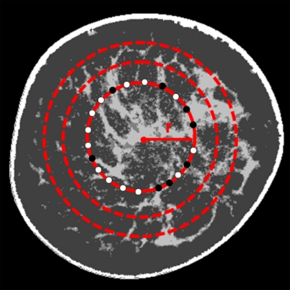
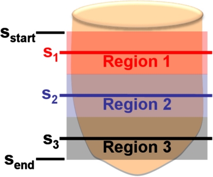
To better understand the fibroglandular distribution within the breast, the distribution of fibroglandular tissue in a coronal bCT image was determined radially. Among the pixels around the circle with a radius r (relative radial distance) originating from the image center of mass, the radial glandular fraction, RGF_si(r), of a coronal bCT image, s_i, was computed as the fraction of pixels marked as fibroglandular tissue (see Fig. 1). The relative radial distance was determined by normalizing the absolute radial distance with the breast radius of the bCT image of interest. One-hundred relative radial distances were considered for each bCT image in this analysis. To obtain a thorough glandular fraction analysis, an entire bCT data set was evenly divided into three regions. Region 1 was the posterior breast section, region 2 was the middle-breast section, and region 3 was the anterior breast section (see Fig. 2). The radial glandular fraction, RGF_n(r), of a breast region, n (1, 2, or 3), was determined by averaging the RGF_si(r) over five images centered about s_n as in Eq. 5,

$${\text{RGF}}_n\left(r\right)=\frac{1}{5}\sum _{s_i=s_n-2}^{s_n+2}{\text{RGF}}_{s_i}\left(r\right),$$ (5)

where s_n is the center image of a breast region, n.

Figure 1.

An illustration to determine the radial glandular fraction of a segmented coronal bCT image, RGF_si(r), is shown. For a radial distance, r, RGF_si(r) is the percentage of the number of pixels marked as fibroglandular tissue (●) and out of the number of pixels marked as fibroglandular tissue or adipose tissue (○).

Figure 2.

The position of three breast regions of a bCT volume bounded by the first good coronal bCT slice (s_start) and the last good coronal bCT slice (s_end) is shown. Region 1 is the posterior section, region 2 is the middle section, and region 3 is the anterior section. The middle slices of the three breast regions are s₁, s₂, and s₃, respectively.

Breast projection areal glandular fraction

The volume glandular fraction was compared with the areal glandular fraction expected from mammography. To properly estimate the areal glandular fraction determined at mammography, a segmented bCT data set was projected in the sagittal orientation to simulate the process of creating a mammographic image. Two steps of projecting through the segmented bCT data set were implemented. A projection of the entire segmented bCT data set was used to delineate the breast border. Secondarily, the number of voxels segmented as fibroglandular tissue along a projection ray through a bCT data set was recorded onto a glandular projection image, I_glandproj(x,y). To simulate the effect of a wide range of radiologists’ visual inspection of breast density at mammography, I_glandproj(x,y) of each bCT data set was then segmented by eight global thresholds (T=0,15.75,31.5,…,110.25 in gray scale value). The breast areal glandular fraction (AGF_Ti) of each bCT data set using a threshold, T_i, was determined using Eq. 6,

$${\text{AGF}}_{T_i}=\frac{A_{gland,T_i}}{A_{gland,T_i}+A_{adipose,T_i}}\cdot 100\mathrm{\%},$$ (6)

where A_gland,Ti is the number of pixels where I_glandproj(x,y)>T_i and A_adipose,Ti is the number of pixels where I_glandproj(x,y)≤T_i.

Data analysis

3D (volumetric) breast assessment

The volumes of adipose tissue and fibroglandular tissue were examined as a function of age. The volume data were binned into 16 age groups (35–37,38–41,…,≥81 years). The mean volume of the respective tissue types (adipose and fibroglandular tissues) and the mean total breast volume were presented as a function of the averaged age for the 16 age groups. The relationship between the volume glandular fraction and age was found using the same age grouping. Similarly, the volume glandular fraction data were categorized into ten breast diameter (D_chestwall) groups according to the 10th percentile D_chestwall(0≤D_chestwall<9.9 cm), the 20th percentile D_chestwall(9.9≤D_chestwall<10.9 cm),…, and >90th percentile D_chestwall(D_chestwall≥15.2 cm). The mean volume glandular fractions of ten D_chestwall groups were found as a function of the averaged D_chestwall for each group. In addition, the relationship between the volume glandular fraction between the affected and unaffected breasts was evaluated for women with no finding, benign, and malignant findings. The distributions of total breast volume and volume glandular fraction for each of the four bra cup sizes (A, B, C, and D) were examined. The relationship between VGF and bra cup size was presented using a box-and-whisker plot (whisker=1.5⋅interquartile range), where the solid dot is the mean VGF with standard error and crosses represent outliers among the VGF of each bra cup size. Box-and-whisker plots were used in similar fashion to present other data in this study. In addition, analysis of variance (ANOVA) and post-hoc multiple comparisons with Bonferroni correction were used to identify significant differences among data groups when applicable. Linear regression was used when appropri-ate. For all the analyses in this study, we considered statistical significance at a two-sided p-value <0.05.

2D (projection and bCT images) breast assessment

The relationship between the breast VGF and the areal glandular fraction (AGF_Ti) was determined using eight global thresholds for all bCT data sets. To characterize the breast composition relative to location in the breast, the GF_n(r) of three breast regions, where n=1 (posterior), 2 (middle), and 3 (anterior), was determined for women with four bra cup size categories (A, B, C, and D). The mean, median, 25th and 75th percentiles, and standard error were reported for all four bra cup sizes. In addition, the areal glandular fractions of coronal bCT images, GF_coronal(z), and sagittal bCT images, GF_sagittal(y), were computed using Eq. 4. Due to the range in breast sizes, the image position (coronal: z direction; sagittal: y direction) was normalized relative to the maximum diameter or length of a bCT data set. Because different slice thicknesses were used in the bCT data sets, cubic spline interpolation (Matlab^©) was applied to the distributions, GF_coronal(z) and GF_sagittal(y), for all bCT data sets to evaluate the areal glandular fraction as a function of relative image position (0,0.005,0.01,…,1.0). For each relative image position, the mean, median, 25th and 75th percentiles, and standard error were computed for bCT data sets of four bra cup sizes.

Breast shape and size assessment

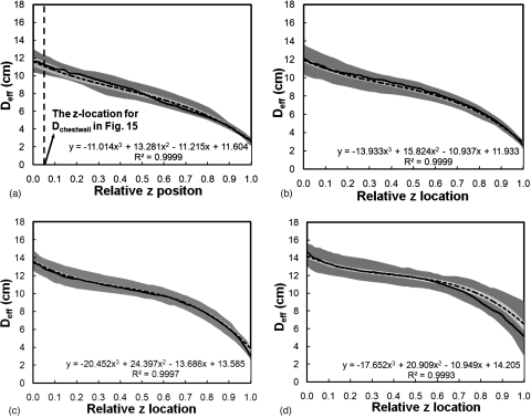
The breast effective diameter as a function of relative posterior-anterior position was computed to characterize the breast shape for each bra cup size. The same cubic interpolation scheme (Sec. 2G2) was applied to the distribution, D_eff(z), at the desired relative position. The mean, median, 25th and 75th percentiles, and standard error were determined. A third-order polynomial was fit to the mean D_eff(z) for women with each bra cup size. The breast length (cm) was determined by the length, in z location, covered by the first good coronal bCT image and the last good coronal bCT image. In addition, the distributions of breast diameter and breast length for four bra cup sizes were evaluated. The total breast volume of the right and left breasts was also compared.

RESULTS

3D (volumetric) breast assessment

The visual assessment of the segmented bCT images in this study demonstrated that 93.1% of the total bCT data sets were rated as good segmentation, 4.1% rated as fair segmentation, and 2.7% as poor segmentation.

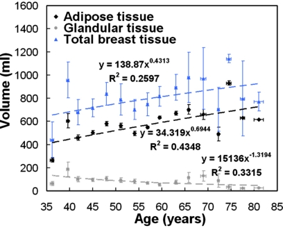
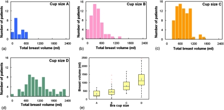
Figure 3 shows the volume of adipose tissue, fibroglandular tissue, and total breast tissues as a function of age. The volume of adipose tissue increases steadily while the volume of fibroglandular tissue decreases gradually as women age. Figure 4 shows that the total breast volume increases as the self-reported bra cup size goes from A to D among 219 women. The mean total breast volumes (± standard error) for bra cup sizes A, B, C, and D were 324.7±44.2, 467.9±36.2, 803.1±33.0, and 1203.7±68.7 ml, respectively.

Figure 3.

The relationship between breast tissue volume and age is illustrated. The dashed line is the line of best fit using a power function. A breast is likely to be composed of more adipose tissue and less fibroglandular tissue as a woman ages. Standard error bars are shown.

Figure 4.

Histogram distributions of the total breast volume (ml) for bra cup sizes (a) A, (b) B, (c) C, and (d) D are shown. (e) A box-and-whisker plot of breast volume as a function of bra cup size is illustrated.

Figure 5 demonstrates the relationship between the VGF of the affected and unaffected breasts among women with no finding, benign, or malignant findings. The VGF of the affected breasts appeared to be slightly higher than that of the unaffected breasts for women with benign or malignant findings, while the women with no finding exhibited almost identical VGF for both breasts. However, the VGFs of the affected breasts and unaffected breasts were not significantly different for the women with benign findings (p=0.40) and malignant findings (p=0.09). Since there might be bias in segmenting bCT data sets with breast cancer, the VGF of the unaffected breast was thought to be a better representation of fibroglandular composition of a woman.

Figure 5.

The correlation of the VGF between the left and right breasts of women is shown for women with (a) no findings. The relationship of the VGF between the affected and unaffected breasts of women with (b) benign findings and (c) malignant findings is shown. The solid line is the line of identity; the dashed line is the fitted linear regression.

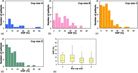
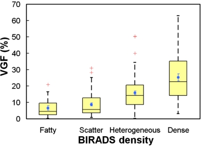
Figure 6 presents the distributions of VGF among women with bra cup sizes A, B, C, and D. The mean VGFs (± standard error) for bra cup sizes A, B, C, and D were 17.7%±3.7%, 19.2%±1.7%, 13.2%±1.2%, and 13.2%±1.3%. The VGF of women with bra cup sizes A and B appears to be slightly larger than that of the women with bra cup sizes C and D. Overall, the mean VGFs of at least two bra cup sizes were significantly different between each other (p=0.01, ANOVA). Post-hoc multiple comparisons with Bonferroni correction suggested that only VGF of bra cup size B was found to be significantly different from that of bra cup sizes C (p=0.0042) and D (p=0.0054). The mean VGFs (± standard error) for the BIRADS categories of fatty, scatter, heterogeneous, and extremely dense were found to be 6.5%±1.4%, 8.8%±1.0%, 15.8%±1.1%, and 25.2%±2.2%, respectively. As shown in Fig. 7, the box-and-whisker plot shows that breasts with higher BIRADS breast density are likely to have higher VGF as well. With each increasing BIRADS category, VGF increased by 5.62% (p<0.001).

Figure 6.

Histogram distributions of the VGF (%) for bra cup sizes (a) A, (b) B, (c) C, and (d) D are shown. (e) A box-and-whisker plot of VGF as a function of bra cup size is shown.

Figure 7.

The graph shows a box-and-whisker plot of volume glandular fraction versus BIRADS density.

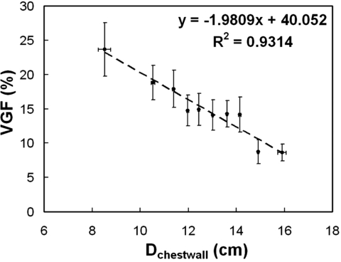
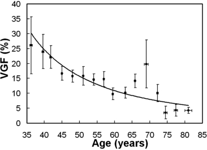
A linear function (r²=0.93) was fit to VGF as a function of breast diameter of the chest wall in Fig. 8. Breasts with larger diameter close to the chest wall were found to have a higher fraction of adipose tissue content. Figure 9 suggests that VGF decrease as women age.

Figure 8.

The relationship between VGF and breast diameter near the chest wall (D_chestwall) is illustrated. Larger breasts tend to have a lower fraction of fibroglandular tissue. Standard error bars are shown.

Figure 9.

The VGF as a function of age is shown. Standard error bars are shown.

2D (projection and bCT image) breast assessment

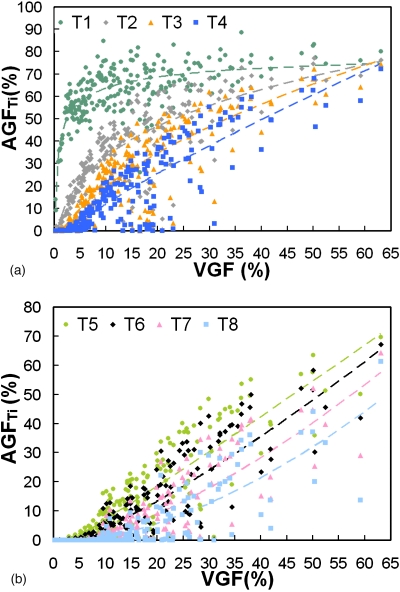
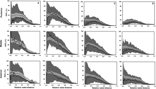
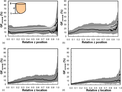
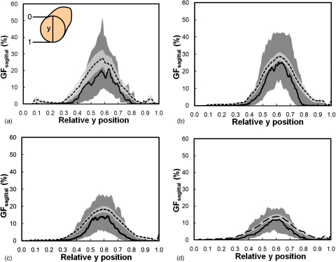
Figure 10 shows that VGF increases with AGF (using eight global thresholds) in a power-law trend. The AGF as a function of VGF using each global threshold was fit using a power function (y=ax^b+c). The coefficients of the power function fit are recorded in Table 2. Figure 11 shows the distribution of radial glandular fraction for three breast regions. For women with bra cup sizes A and B, fibroglandular tissue tends to locate in the center portion of the breast evenly throughout the three breast regions. For women with cup sizes C and D, fibroglandular tissue is concentrated more in the breast center toward the breast anterior regions. Figures 1213 display the distributions of GF_coronal(z) and GF_sagittal(y) for each bra cup size. The dashed line is the mean GF_p, and the solid line is the median GF_p. The darker shade covers the range of 25th percentile below and 75th percentile above the median. The lighter shade covers the range of standard error above and below the mean. Across all four bra cup sizes, GF_coronal(z) was found to be relatively homogeneously distributed but increased dramatically toward the nipple, as shown in Fig. 12. Figure 13 shows that GF_sagittal(z) is concentrated heavily in the middle of the breast, with a slight offset (∼10%) inferiorly.

Figure 10.

The areal glandular fraction is shown versus the volume glandular fraction using a threshold level (gray scale value) where (a) T1=0, T2=15.75, T3=31.50, and T4=47.25 and (b) T5=63, T6=78.75, T7=94.50, and T8=110.25.

Table 2.

The coefficients of the power function (y=ax^b+c) fit to AGF as a function VGF using eight global thresholds in Fig. 10.

Global threshold	a	b	c	r2
0.00	−52.0122	−0.3221	88.3594	0.5619
15.75	34.4143	0.2744	−31.7009	0.6931
31.50	8.3916	0.5645	−10.9426	0.7312
47.25	2.6417	0.8236	−5.6304	0.7447
63.00	0.9318	1.0571	−3.6154	0.7545
78.75	0.3509	1.2709	−2.5259	0.7462
94.50	0.1210	1.4953	−1.7542	0.7208
110.25	0.0384	1.7281	−1.1792	0.6715

Figure 11.

The radial glandular fraction is plotted as a function of relative radial distance for women with bra cup sizes A, B, C, and D for three breast regions (posterior, middle, and anterior). The dashed line is the mean RGF_n and the solid line is the median RGF_n. The darker shade covers the range of 25th percentile below and 75th percentile above the median. The lighter shade covers the range of standard error above and below the mean.

Figure 12.

The glandular fraction of coronal bCT slices is shown versus the relative z position for women with bra cup sizes (a) A, (b) B, (c) C, and (d) D. The direction of z position relative to a bCT volume data set is illustrated in A, where 0 is posterior and 1 is anterior. The dashed line is the mean GF_coronal and the solid line is the median GF_coronal. The darker shade covers the range of 25th percentile below and 75th percentile above the median. The lighter shade covers the range of standard error above and below the mean.

Figure 13.

The glandular fraction of sagittal bCT slices versus the relative y position for women is shown for breasts with bra cup sizes (a) A, (b) B, (c) C, and (d) D. The direction of y position relative to a bCT volume data set is illustrated in A, where 0 is superior and 1 is inferior. The dashed line is the mean GF_sagittal and the solid line is the median GF_sagittal. The darker shade covers the range of 25th percentile below and 75th percentile above the median. The lighter shade covers the range of standard error above and below the mean.

Breast shape and size assessment

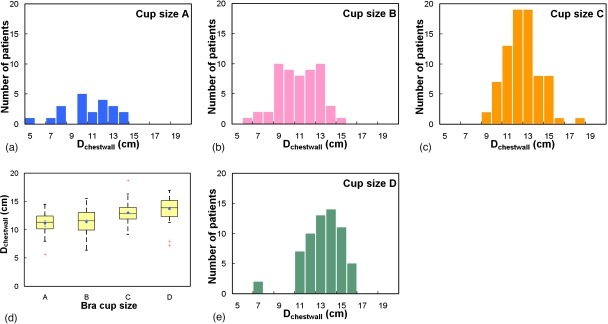
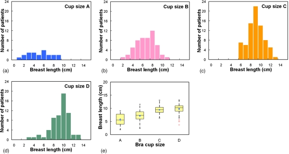
Across all four bra cup sizes, Fig. 14 shows that the breast shape can be generally characterized by the breast effective diameter, which gradually decreases from posterior to anterior. A third-order polynomial described those trends well (r²>0.9993). The starting D_eff(z) of a breast increased as a function of bra cup sizes. In more detail, Fig. 15 shows that the mean breast diameter (D_chestwall) slightly increased with bra cup sizes, where D_chestwall was measured at the relative z location indicated by the dashed line in Fig. 14a. The mean breast diameters (± standard error) for bra cup sizes A, B, C, and D were 11.1±0.5, 11.4±0.3, 13.0±0.2, and 13.7±0.2 cm, respectively. The box-and-whisker plot in Fig. 15e confirmed the observation in Figs. 15a, 15b, 15c, 15d that breasts with larger diameter corresponded to larger bra cup sizes. In addition, Fig. 16 illustrates that breast length appears to increase slightly with bra cup size. The mean breast lengths (± standard error) for bra cup sizes A, B, C, and D were 5.7±0.5, 7.1±0.3, 9.4±0.2, and 9.7±0.2 cm, respectively. The box-and-whisker plot in Fig. 16e confirmed that women with larger bra cup size tend to have longer breast length. Lastly, the right breast volume was found to be comparable to the left breast volume (slope=0.995). A paired student’s t test confirmed that the right breast volume was not significantly different from the left breast volume (p=0.17). A total of 48.7% of all the breasts in this analysis were ones with the benign or malignant findings.

Figure 14.

The breast effective diameter versus the relative z position is shown for women with bra cup sizes (a) A, (b) B, (c) C, and (d) D. The dashed line is the mean D_eff and the solid line is the median D_eff. The darker shade covers the range of 25th percentile below and 75th percentile above the median. The lighter shade covers the range of standard error above and below the mean. A third-order polynomial was fit to the mean breast diameter profile for each bra cup size.

Figure 15.

Histogram distributions of the breast diameter (D_chestwall) near the chest wall is shown for women of bra cup sizes (a) A, (b) B, (c) C, and (d) D. (e) A box-and-whisker plot of breast diameter is shown as a function of bra cup size.

Figure 16.

Histogram distributions of the breast length (cm) are shown for bra cup sizes (a) A, (b) B, (c) C, and (d) D. (e) A box-and-whisker plot of breast length as a function of bra cup size is illustrated.

DISCUSSION

In this study, a comprehensive analysis of breast composition and breast shape was performed to characterize breast anatomy in women of different ages and with different breast sizes. The data presented provide anatomically grounded information to guide the construction of physical or simulated breast phantoms. In addition to the detailed description of breast geometry, the distribution of fibroglandular tissue in the breast was reported using both 2D and 3D metrics.

It is important to note that the BIRADS density determined at mammography tends to overestimate the glandular fraction due to the overlap of fibroglandular tissue distribution from breast compression and the projection imaging geometry. This study found that BIRADS densities overestimate the true volume glandular fraction by approximately 1.9-fold for fatty breasts, 4.2-fold for scattered breasts, 4.0-fold for heterogeneous breasts, and 3.5-fold for extremely dense breasts. The findings also confirm the overestimation of breast density at mammography for the “average” breast, which has been shown to be 19.3% but not the commonly assumed 50%.¹¹ However, Figs. 710 can be used to estimate the VGF for a given mammographic BIRADS category or AGF (assuming no breast compression). Furthermore, the coefficients in Table 2 allow one to estimate VGF from AGF for a variety of segmentation thresholds. The global thresholding scheme (Sec. 2F) used in estimating breast density at 2D projection images is crude but represents the subjective visual thresholding by a wide variety of observers. Further studies should establish where most radiologists fall in this range of thresholds. The effect of breast compression on VGF-AGF relationship must also be explored.

The study results also guide the construction of a physical or simulated breast phantom, accounting for age and breast size (volume, breast diameter, and length). Previous studies^{12, 13} have suggested that the breast density decreases steadily with increasing age. Figures 39 confirm this observation. Breast diameter, breast length, VGF, and fibroglandular tissue distribution appear to change with bra cup size. Bra cup size may be a rough classification of breast size with respect to these metrics. Moreover, Figs. 111213 suggest that fibroglandular tissue generally originates from the breast nipple and locate heavily in the center part of a breast in three dimensions. Based on mammographic images, a previous study¹⁴ suggests that fibroglandular tissue is preferentially located in the center portion of a breast in both medial-lateral and cranial-caudal directions. The finding in this study suggests a similar trend in fibroglandular tissue distribution in three dimensions. Combining VGF, RGF_n, GF_coronal, and GF_sagittal from this study, a 3D probability map of fibroglandular tissue within a breast of a given breast size can be generated. At certain breast locations, the mean RGF_n, GF_coronal, or GF_sagittal is larger than its 75th percentile due to outliers among the data. Breast phantoms calibrated to age, size, and fibroglandular tissue distribution may be useful for observer performance studies in breast imaging and Monte Carlo simulation of x-ray dosimetry.

Limitations of this study include the bCT protocol in scanning larger patients. For women with bra cup size D or larger, the breast is confined anteriorly to be within the field of view. In doing so, breast length may be slightly underestimated. The wide range of chest wall and axillary coverage in the bCT images may poorly characterize breast tissue distribution in these regions, leading to slight inaccuracy in VGF and AGF.

Despite these limitations, this work presents a description of the breast using the largest available set of images acquired with breast CT, to our knowledge. This study describes the relationship between the 2D and 3D representations of fibroglandular fraction and the overestimation when using BIRADS density. A number of breast anatomical metrics were introduced and characterized in detail, describing breast shape, breast diameter and length, radial breast glandular fraction in three breast regions, and glandular fraction along two orthogonal planes of the breast as a function of patient age and bra cup size. Three-dimensional breast phantoms can be accurately generated using the breast anatomical metrics developed in this study.

References

- Bochud F. O., Abbey C. K., and Eckstein M. P., “Statistical texture synthesis of mammographic images with clustered lumpy backgrounds,” Opt. Express 4(1), 33–43 (1999). 10.1364/OE.4.000033 [DOI] [PubMed] [Google Scholar]
- Kallergi M., Gavrielides M. A., Berman C. G., Kim J. J., and Clark R. A., “Simulation model of mammographic calcifications based on the American College of Radiology Breast Imaging Reporting and Data System or BIRADS,” Acad. Radiol. 5(10), 670–679 (1998). 10.1016/S1076-6332(98)80561-8 [DOI] [PubMed] [Google Scholar]
- Lado M. J., Tahoces P. G., Souto M., Mendez A. J., and Vidal J. J., “Real and simulated clustered microcalcifications in digital mammograms. ROC study of observer performance,” Med. Phys. 24(9), 1385–1394 (1997). 10.1118/1.598027 [DOI] [PubMed] [Google Scholar]
- Lefebvre F., Benali H., Gilles R., and Di Paola R., “A simulation model of clustered breast microcalcifications,” Med. Phys. 21(12), 1865–1874 (1994). 10.1118/1.597186 [DOI] [PubMed] [Google Scholar]
- Nappi J. J. and Dean P. B., “Mammographic feature generator for evaluation of image analysis algorithms,” Proc. SPIE - Int. Soc. Opt. Eng. 3034, 911–918 (1997). [Google Scholar]
- Bakic P. R., Albert M., Brzakovic D., and Maidment A. D. A., “Mammogram synthesis using a 3D simulation. 1. Breast tissue model and image acquisition simulation,” Med. Phys. 29(9), 2131–2139 (2002). 10.1118/1.1501143 [DOI] [PubMed] [Google Scholar]
- Bliznakova K., Bliznakov Z., Bravou V., Kolitsi Z., and Pallikarakis N., “A three-dimensional breast software phantom for mammography simulation,” Phys. Med. Biol. 48(22), 3699–3719 (2003). 10.1088/0031-9155/48/22/006 [DOI] [PubMed] [Google Scholar]
- Boone J. M., Kwan A. L., Seibert J. A., Shah N., Lindfors K. K., and Nelson T. R., “Technique factors and their relationship to radiation dose in pendant geometry breast CT,” Med. Phys. 32(12), 3767–3776 (2005). 10.1118/1.2128126 [DOI] [PubMed] [Google Scholar]
- Yang K., Kwan A., Burkett G., and Boone J. M., “Hounsfield units calibration with adaptive compensation of beam hardening for a dose limited breast CT system,” in American Association of Physicists in Medicine 28th Annual Meeting, Orlando, FL, 2006.
- Packard N. and Boone J. M., “Glandular segmentation of cone beam breast CT volume images,” Proc. SPIE 6510(1), 651038 (2007). 10.1117/12.713911 [DOI] [Google Scholar]
- Yaffe M. J., Boone J. M., Packard N., Alonzo-Prouix O., Huang S. Y., Peressotti C. L., Al-Mayah A., and Brock K., “The myth of the 50-50 breast,” Med. Phys. 36(12), 5437–5443 (2009). 10.1118/1.3250863 [DOI] [PMC free article] [PubMed] [Google Scholar]
- Kopans D. B., Breast Imaging, 3rd ed. (Lippincott-Raven, Philadelphia, PA, 2007), pp. 350 and 351. [Google Scholar]
- Stomper P. C., Dsouza D. J., DiNitto P. A., and Arredondo M. A., “Analysis of parenchymal density on mammograms in 1353 women 25–79 years old,” AJR, Am. J. Roentgenol. 167(5), 1261–1265 (1996). [DOI] [PubMed] [Google Scholar]
- Astley S. M. and Caulkin S., “The generation of synthetic spiculated lesions in digital mammograms using statistical models,” Radiology 225, 645–645 (2002). [Google Scholar]