Abstract
The illustrations in biomedical publications often provide useful information in aiding clinicians’ decisions when full text searching is performed to find evidence in support of a clinical decision. In this research, image analysis and classification techniques are explored to automatically extract information for differentiating specific modalities to characterize illustrations in biomedical publications, which may assist in the evidence finding process.
Global, histogram-based, and texture image illustration features were compared to basis function luminance histogram correlation features for modality-based discrimination over a set of 742 manually annotated images by modality (radiological, photo, etc.) selected from 2004-2005 issues of the British Journal of Oral and Maxillofacial Surgery. Using a mean shifting supervised clustering technique, automatic modality-based discrimination results as high as 95.57% were obtained using the basis function features. These results compared favorably to other feature categories examined. The experimental results show that image-based features, particularly correlation-based features, can provide useful modality discrimination information.
1. Introduction
Querying publications to find relevant information regarding a clinical situation that can assist a clinician can be a challenging task. There are many types of information present in publications that can be useful to clinicians. In previous research, automatic illustration identification was investigated for illustrations in medical publications to assist in providing information that could aid clinicians evaluate the usefulness of a publication for a particular clinical situation [1,2]. Specific modalities were examined for illustration classification based on providing delimiters for the types of information present within the medical publication [1,2]. Our research group has also explored image features to foster the finding of relevant images that appear in publications and machine learning- and pipeline information retrieval-based approaches that facilitate the leveraging of information contained in the text and images [3]. Experimental results for this research showed the potential to obtain image annotation and retrieval accuracy acceptable for providing clinical evidence, given sufficient training data [3]. In this research, numerous types of image descriptors are investigated for modality-based illustration classification. The descriptors examined build upon features used in Content Based Image Retrieval (CBIR) systems and in medical image analysis.
In this research, we have studied various techniques for Content Based Image Retrieval (CBIR) systems and investigated a number of features for classifying images extracted from biomedical journal articles into categories by modality, anatomy, and evidence-based practice Content Based Image Retrieval.
An overview of some existing features and techniques used in image retrieval systems is presented here, which provided the basis for the features and classification techniques investigated in this research. For CBIR, color, shape and texture features of an image are widely used to measure similarity between images [1-11]. Some other approaches include wavelet decomposition and analysis [12,13], hierarchical [14], user interest modeling [15], and multi-modal [1,2,16]. In order to illustrate specific features, a multi-resolution, multi-grid framework has been applied to localized color moment and Gabor filter features as well as the calculation of shape features based on edge information obtained from gradient vector flow fields [4]. Texture and grey level features have also been utilized in CBIR systems [9]. In particular, grey level features based on histogram analysis and grey level distribution such as mean, standard deviation, root mean square, skewness, and Kurtosis. For this study, texture measures based on grey level co-occurrence and LAWS filters have been explored [9]. A combination of color and texture features with different weights has been investigated [13]. The color histogram was generated using the HSV representation of the image and a weighting scheme was applied to each pixel based on hue and saturation values. The texture features were extracted using Haar or Daubechies’ wavelet.
In this research, basis function correlation features computed from the luminance histogram are compared to other global and texture measures for discrimination of images as modality-based illustration classification indices. These basis function correlation features have been explored in dermatology imaging research to provide grey level distribution information for skin lesion discrimination [17]. The measures investigated are applied to a set of medical publication illustrations and modalities examined in previous research [1]. The remainder of the paper is organized as follows: 1) description of the features and feature groups investigated, 2) modality-based illustration experiments performed, 3) results and discussion, and 4) conclusions.
2. Methodology
2.1 Data Set Examined
For this research, a data set of images encompassing nine different modalities was selected from the British Journal of Oral and Maxillofacial Surgery, which has been used in previous research [1]. The rationale for choosing this journal to obtain images for the experimental data set is that it is an area of expertise for one of the co-authors, and the images from this journal are representative of the specialties that could benefit from visual information obtained early in the information retrieval process. For obtaining the data set, two authors of this paper studied 2004 and 2005 online issues of the journal and downloaded full-size images and HTML text of articles and short communications containing images. The images were manually annotated and cross validated for their modality and utility in finding clinical evidence. In this research, image features are investigated for modality-based classification using supervised machine learning techniques as a means to determine the feasibility of automatic image annotation based on clinical utility. In previous research, analyzing 2006 issues of the British Journal of Oral and Maxillofacial Surgery, it was observed that the aspects of the clinical scenario such as patient/problem, intervention/comparison, and outcome for the clinical tasks of diagnosis and therapy typically are often illustrated [1].
Table 1 presents the nine categories for image modality explored in this research. The rationale for selecting these modalities is given in [1]. Overall, the experimental data set consisted of 742 images. Table 2 contains the distribution of the images in the different categories for image modality given in Table 1. Figures 1-9 provide examples of images from each modality.
Table 1.
Categories for Image Modality
| Category | Definition |
|---|---|
| Chart / Graph | A geometric diagram consisting of dots, lines, and bars. |
| Drawing | A hand drawn illustration |
| Flowchart | A symbolic representation of sequence of activities. |
| Form | A compilation of textual data and/or drawings related to patient and/or clinical process. |
| Histology | An image of cells and tissue on the microscopic level. |
| Photograph | Picture obtained from a camera |
| Radiology | A 2D view of an internal organ or structure (includes X-ray, CT, PET, MRI, ultrasound) |
| Table | Data arranged in a grid |
| Mixed | Images combining modalities (e.g., drawings over an x-ray) |
Table 2.
Number of Images from Each Category for Image Modality Case
| Category | Number of Images Used in Study |
|---|---|
| Chart / Graph | 108 |
| Drawing | 68 |
| Flowchart | 7 |
| Form | 11 |
| Histology | 134 |
| Photograph | 252 |
| Radiology | 108 |
| Table | 46 |
| Mixed | 8 |
Figure 1.
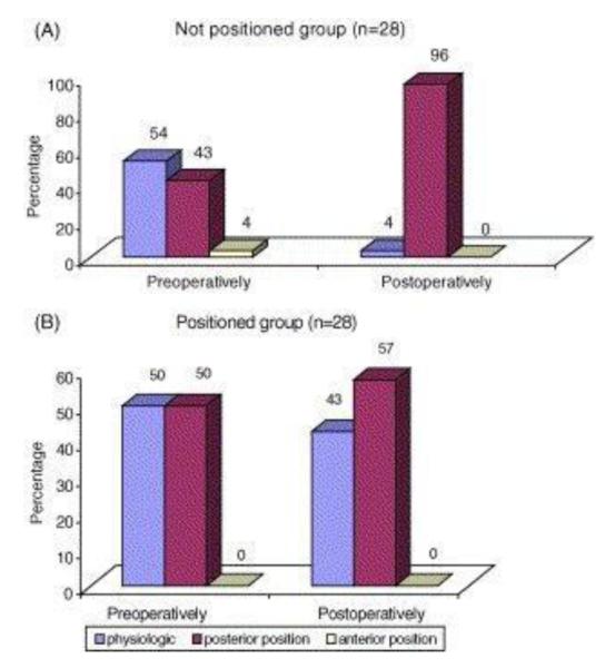
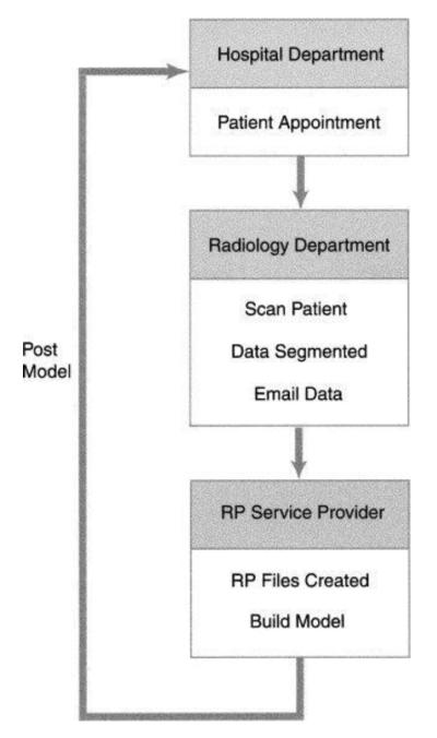
Example image for chart/graph modality (reproduced with permission [18]).
Figure 9.
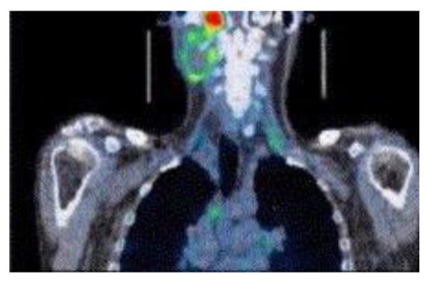
Example image for mixed modality (reproduced with permission [26]).
2.2 Features and Feature Groups Investigated
The global, texture-based, and basis function correlation measures investigated are presented in this section. These features were divided into three groups, labeled as Group 1, Group 2, and Group 3, based on the feature type. Modality-based classification algorithm investigation and development were explored for the image set with categories and numbers of images as provided in Tables 1 and 2, respectively. The Group 1 features included the following global features: 1) the standard deviation of the standard deviation computed over the columns of the image. Let stdColRed, stdColGreen, and stdColBlue denote these standard deviation features computed for the red, green, and blue planes, respectively, for a color image. stdColRed, stdColGreen, and stdColBlue are the same values for grayscale images. These features were examined to evaluate the change in contrast across the image. 2) the ratio of the pixels in the image in which the green value is less than the red value and the green value is less than the blue value, given as pixelsG, to the area or size of the image. The ratio is denoted as percentG and is given as follows:
| (1) |
This feature provides a basic measure of the greenness of the image. 3) the ratio of the pixels in the image with luminance value greater than or equal to 250, given as pixelsWhite, to the area/size of the image. The ratio is given as percentWhite and expressed as:
| (2) |
This feature gives a whiteness metric which is prevalent in images from several modality categories. 3) several descriptors computed from the L histogram of the image (from the LUV color space). The first of the descriptors is the most frequently occurring L value in the image, denoted as mostFrequentGray. If more than one value had the same (maximum) frequency of occurrence, the lowest of those L values was chosen. The second of the descriptors is the ratio of the number of pixels with the most frequently occurring L value, given as the numberPixelsMostFrequentGray, to the area/size of the image. The ratio is defined as percentMostFrequent in equation form as
| (3) |
The third descriptor is the average L value over the image, given as avgGray. The fourth descriptor is the standard deviation L value over the image, labeled as stdGray. Several studies have cited descriptors from the LUV color space for content-based image retrieval. 4) The square root of the area/size of the image, denoted as sqrtArea. This feature was used to see if image area/size for the different categories was a distinguishing characteristic. 5) The ratio of the pixels in the image with luminance values between 50 and 150 (inclusive), labeled as pixels50to150, to the area/size of the image. The ratio is defined as
| (4) |
The goal with this feature is to distinguish the images within particular categories as being bright (white), dark or moderate. 6) The ratio of the sum of the absolute differences between the red and green values and the red and blue values for each pixel in the image to the area/size of the image. Let (R(i,j),G(i,j),B(i,j)) denote red, green, and blue values at pixel location (i,j), respectively. The ratio is given as sumDiff and is defined in the following equation
| (5) |
This feature provides a basic homogeneity measure. 7) The ratio of the pixels in the image with luminance value less than or equal to 30, labeled as pixelsDark, to the area/size of the image and is expressed as
| (6) |
8) Several color/luminance count indices. The first index is computed as the square root of the number of luminance histogram bins with counts greater than or equal the area of the image times 0.001 (0.001 is chosen to discount histogram bins with very small counts), denoted as colorCount. The second index is computed as the square root of the number of luminance histogram bins with counts greater than 0, denoted as colorCount1. The third index is computed as the square root of the number of luminance histogram bins with counts greater than or equal the area of the image times 0.01, denoted as colorCount2. colorCount, colorCount1, and colorCount2 provide three grayscale counting metrics for quantifying grayscale variation within the images in different categories. 9) Estimates of the fractal dimension [27]. The first estimate of the fractal dimension is based on second order discrete derivatives computed column-wise over the image, given as fractDim1. The second estimate of the based on second order discrete derivatives computed column-wise over the image using symlets (sym5), labeled as fractDim2. Fractal dimension was investigated here as a global image measure.
The Group 2 features investigated included the basis function features computed based on correlating the luminance histogram with a set of six weight density distribution (WDD) functions [28], i.e. basis functions. Twelve WDD-based features are computed. Each of the WDD functions is decomposed into 256 discrete points for point-to-point correlation with the luminance histograms of the images. Let W1 denote the WDD function in Figure 1 (a), W2 denote the WDD function in Figure 1 (b) and so on. For an image, six WDD features (fΓ1, …,fΓ,6) are computed using the luminance histogram Γ according to the expression
| (7) |
The WDD functions were adjusted to have 256 points that were point-to-point correlated and multiplied with the WDD functions, with the feature values as the sums of the point-to-point multiplications. Six additional features (fΓ,7, …, fΓ,12) are computed by correlating the six WDD functions with the sequence of absolute differences between of the histogram frequencies for consecutive luminance values as
| (8) |
The WDD features provide different ways of quantifying the variation, symmetry and distribution of gray values within the images.
The Group 3 features examined in this study were texture measures based on the Generalized Gray Level Spatial Dependence Models for Texture using the implementation given in [29]. The following features were computed with the luminance image for finding the gray level co-occurrence matrix with a radius of 1. This means that gray level co-occurrence was found for each pixel (i,j) over the 3×3 neighborhood of (i,j). Let Q represent the gray level co-occurrence, K represent the maximum intensity in the image with k = 1, …, K, and S provide the neighborhood count (maximum of 9=3×3) with s = 1, …, S. The features calculated from the luminance image include:
| (9) |
| (10) |
| (11) |
| (12) |
| (13) |
| (14) |
| (15) |
| (16) |
| (17) |
For the expressions above , mr, and mc are the row and column means for Q, respectively, and or and oc are the row and column standard deviations for Q, respectively. The features above include entropy, contrast, homogeneity, correlation, energy uniformity, and inverse difference moments. The goal with these features is to provide rotation and size invariant global texture measures using the entire image as the region of interest for these feature calculations.
All features from Groups 1-3 presented above were implemented in Java and were computed over the 742 image data set. The feature vectors for Groups 1-3 are summarized as follows. Group 1 includes the general features with stdColRed, stdColGreen, stdColBlue, percentG, percentWhite, percentMostFrequent, sqrtArea, avgGray, stdGray, percentMiddle, sumDiff, percentDark, colorCount, fractDim1. Group 2 consists of the WDD features (fΓ1, …, fΓ,12). Group 3 includes the texture features T1-T9. The features were divided into these groups to avoid large feature vectors and to evaluate and compare the classification results of the different types of features.
2.3 Image Classification for Modality Cases
In order to evaluate the discrimination capability of the different features groups, radial clustering, and a modification for a gradient density function clustering-based [30] classification techniques were examined. Both algorithms were implemented in Java and are described below. For image classification, each category of the image set (given in Table 1) was partitioned using 90% of the images within the category for the training set and the remaining 10% of the images within the category for the test set. Feature normalization was performed using a fuzzy set approach. Using the training set for each feature, the minimum and maximum feature values, denoted as m and x, respectively, are determined. Let A denote the fuzzy set for a particular feature. The membership function for A is labeled as μA(p) for feature value p and is defined as . μA is found for all features for each category from the training set of images. All feature values for each training and test set image are normalized using μA found for the respective features. The normalized training feature vectors are used to find cluster centers for the radial clustering and gradient density function clustering-based methods.
The radial clustering method determines cluster centers from the training data for each modality category by specifying an intra-cluster distance, i.e. radius for the cluster, δ. For each category, cluster centers are determined from the training data using the following steps. First, select an initial cluster center as the first normalized training feature vector for a specified category. Second, for the next normalized training feature vector, compute the Euclidean distance to the initial cluster center. If the distance is greater than δ, create a new cluster and initialize its cluster center as the current normalized feature vector. Otherwise, select the cluster for membership for which the feature vector has a minimum Euclidean distance. The cluster center for the selected cluster is updated as the mean feature vector of all feature vectors belonging to the cluster. Third, repeat step 2 for all training feature vectors for the specified category. Fourth, repeat steps 2 and 3 until the cluster centers do not change for an iteration through the training data or a specified number of iterations through the training data, whichever requires fewer iterations through the training data.
The gradient density function clustering-based technique (also referred to as mean shift clustering method) is implemented based on the algorithm presented in [30]. This technique automatically determines the number of cluster centers from the training set and is applied to test set for classification into the different categories. As part of this technique, there is a bandwidth parameter (α) which is used for data partitioning for cluster and number of cluster determination.
In order to classify each test image, the following steps were performed. First, the Euclidean distance from the test image feature vector to each of the cluster centers for a specified category is computed. Second, the minimum Euclidean distance is found and is used to represent the distance to the specified category. Third, steps 1 and 2 are repeated for all categories. Fourth, the test image feature vector is assigned to the category with the minimum Euclidean distance. These steps were applied to classifying each test image based on the feature vectors and clusters determined for Groups 1, 2, and 3.
3. Experiments Performed
In order to evaluate the different feature groups, fifty randomly generated training and test sets were used for the data set described in section 2.1. Each training set consists of 90% of the image data feature vectors for each category, and each corresponding test set contains the remaining 10% of the image data feature vectors for each category. The image data feature vectors includes the features computed from Groups 1-3. Radial clustering and gradient density function clustering-based classifiers were used to evaluate the different feature groups over the 25 training/test sets.
4. Experimental Results and Discussion
For radial clustering, δ = 0, 0.5, 1.0, 5.0, 10.0, and 30.0 were examined for one iteration through the training data. Table 3 presents the test results using the radial clustering method for δ = 0.5 for feature groups 1-3. The test results for each of the 25 randomly generated training/test sets are given with the mean and standard deviation for the respective feature groups. Table 4 provides the average number of cluster centers determined from the training data for δ = 0.5 for each category over the 25 randomly generated training/test sets. These are the cluster centers used for classifying the image feature vectors into the different categories. Table 5 presents the average and standard deviation test results over the 25 randomly generated training/test sets based on the features computed for Groups 1-3 using the radial clustering method with δ = 0, 0.5, 1.0, 5.0, 10.0, and 30.0.
Table 3.
Test results using radial clustering method for δ = 0.5 for feature groups 1-3 for 25 training/test sets are presented with mean and standard deviation.
| Training/Test Set | % Correct Test Image Results for All Categories – Group 1 Features |
% Correct Test Image Results for All Categories – Group 2 Features |
% Correct Test Image Results for All Categories – Group 3 Features |
|---|---|---|---|
| 1 | 88.00 | 96.00 | 96.00 |
| 2 | 88.00 | 97.33 | 96.00 |
| 3 | 89.33 | 96.00 | 92.00 |
| 4 | 88.00 | 96.00 | 98.67 |
| 5 | 82.67 | 90.67 | 90.67 |
| 6 | 86.67 | 94.67 | 96.00 |
| 7 | 88.00 | 97.33 | 97.33 |
| 8 | 80.00 | 92.00 | 92.00 |
| 9 | 92.00 | 96.00 | 96.00 |
| 10 | 82.67 | 93.33 | 94.67 |
| 11 | 85.33 | 98.67 | 96.00 |
| 12 | 86.67 | 96.00 | 92.00 |
| 13 | 92.00 | 96.00 | 93.33 |
| 14 | 80.00 | 96.00 | 92.00 |
| 15 | 84.00 | 93.33 | 93.33 |
| 16 | 80.00 | 94.67 | 93.33 |
| 17 | 86.67 | 96.00 | 97.33 |
| 18 | 85.33 | 97.33 | 93.33 |
| 19 | 81.33 | 94.67 | 89.33 |
| 20 | 80.00 | 94.67 | 92.00 |
| 21 | 93.33 | 94.67 | 94.67 |
| 22 | 89.33 | 97.33 | 96.00 |
| 23 | 88.00 | 96.00 | 94.67 |
| 24 | 93.33 | 98.67 | 97.33 |
| 25 | 80.00 | 96.00 | 92.00 |
| Average | 86.03 | 95.57 | 94.24 |
|
Standard
Deviation |
4.34 | 1.87 | 2.40 |
Table 4.
Average number of cluster centers generated from radial clustering method for δ = 0.5 over 25 randomly generated training/test sets.
| Category | Average Number Clusters – Group 1 |
Average Number Clusters – Group 2 |
Average Number Clusters – Group 3 |
|---|---|---|---|
| Chart / Graph | 38.84 | 17.96 | 9.32 |
| Drawing | 39.88 | 23.80 | 15.48 |
| Flowchart | 4.56 | 6.00 | 4.68 |
| Form | 10.00 | 8.24 | 4.68 |
| Histology | 79.76 | 37.64 | 10.72 |
| Photograph | 146.76 | 28.72 | 17.08 |
| Radiology | 55.52 | 25.40 | 15.12 |
| Table | 12.00 | 12.48 | 6.60 |
| Mixed | 7.00 | 6.48 | 6.36 |
Table 5.
Summary average and standard deviation test results over 25 training/test sets using radial clustering method for δ = 0, 0.5, 1.0, 5.0, 10.0, and 30.0.
| Group 1 | Group 2 | Group 3 | |
|---|---|---|---|
|
Average %
Correct Test Results |
|||
| δ = 0 | 86.03 | 95.57 | 94.24 |
| δ = 0.5 | 84.91 | 95.41 | 85.92 |
| δ = 1.0 | 84.32 | 95.31 | 78.83 |
| δ = 5.0 | 76.21 | 93.39 | 70.24 |
| δ = 10.0 | 72.16 | 91.73 | 68.53 |
| δ = 30.0 | 57.71 | 90.88 | 70.29 |
|
Standard
Deviation Test Results |
|||
| δ = 0 | 4.34 | 1.87 | 2.40 |
| δ = 0.5 | 4.21 | 1.93 | 4.90 |
| δ = 1.0 | 3.93 | 2.18 | 6.27 |
| δ = 5.0 | 5.96 | 3.23 | 4.42 |
| δ = 10.0 | 6.35 | 2.55 | 4.75 |
| δ = 30.0 | 9.16 | 2.82 | 5.79 |
Inspecting the results from Tables 3-5, several observations can be made. First, the δ = 0 case corresponds to a nearest neighbor classifier. From the training mode, the number of cluster centers equals the number of training feature vectors. Increasing values of δ increases the number of feature vectors belonging to each cluster, thereby, reducing the number of cluster centers. Second, the Group 2 features computed by correlating the basis functions given in Figure 1 with the luminance histogram of the image provide the highest overall classification into the different categories. The classification results are as high as 95.57% for δ = 0 (nearest neighbor case) and as low as 90.88% for δ = 30.0. These results show that these features generalize reasonably well as the number of clusters increase for representing the different categories of the data set investigated in this study. Table 6 provides the average number of cluster centers determined from the training data for δ = 30.0 for each category over the 25 randomly generated training/test sets. From Tables 4 and 6, the number of clusters substantially declines from δ = 0.5 to δ = 30.0 for feature Groups 1-3. However, the average test correct classification rates do not significantly decline with 95.41% for δ = 0.5 and 90.88% for δ = 30.0. Overall, the Group 2 feature results compare quite favorably with the Group 1 and Group 3 feature sets, particularly with increasing values of δ, i.e. increasing numbers of cluster centers. Third, the average test results for δ = 0 (nearest neighbor case) for feature Groups 1-3 are higher than for the other values of δ. Because many of the publications used in generating the image set may consist of similar images which may be separated into the training and test sets, which could promote higher classification using the nearest neighbor case from the radial clustering method. Fourth, three types of features have been investigated in this study. The Group 1 features consist of global image descriptors such as thresholding, color counting, statistical measures such as standard deviation and most frequently occurring gray level, and Fractal dimension. As global measures, these features do not provide context to the distribution of gray level information within the images for the different categories. The Group 3 features provide texture measures for distinguishing the different modality categories. The Group 2 features quantify the luminance value distribution for the different categories based on correlating the luminance histograms with a set of basis functions to provide global measures for distinguishing the different categories. The basis functions used in this study, shown in Figure 1, are zero sum except for (d). Correlation of the luminance histogram with these basis functions quantizes the global gray level distribution within the different categories. The experimental results show that the correlation features provide effective similarity measures for images within each category. Furthermore, experimental results show that clustering of these features yield strong discriminators for the different categories examined in this study. Finally, Tables 7-9 show the average correct results over the 25 test sets in confusion matrix form for the features for Groups 1-3, respectively, for δ = 1.0.
Table 6.
Average number of cluster centers generated from radial clustering method for δ = 30.0 over 25 randomly generated training/test sets.
| Category | Average Number Clusters – Group 1 |
Average Number Clusters – Group 2 |
Average Number Clusters – Group 3 |
|---|---|---|---|
| Chart / Graph | 1.00 | 5.96 | 1.92 |
| Drawing | 1.08 | 5.12 | 1.44 |
| Flowchart | 1.92 | 3.24 | 1.04 |
| Form | 1.96 | 5.68 | 1.64 |
| Histology | 1.24 | 4.88 | 1.00 |
| Photograph | 2.32 | 7.84 | 1.00 |
| Radiology | 1.44 | 6.80 | 1.00 |
| Table | 1.96 | 3.32 | 1.96 |
| Mixed | 2.72 | 3.72 | 1.04 |
Table 7.
Average confusion matrix test results for Group 1 for δ = 1.0 from radial clustering method.
| Category\Category | 1 | 2 | 3 | 4 | 5 | 6 | 7 | 8 | 9 |
|---|---|---|---|---|---|---|---|---|---|
| 1 | 10.44 | 0.48 | 0.04 | 0 | 0 | 0 | 0 | 0.04 | 0 |
| 2 | 0.76 | 5.84 | 0 | 0 | 0.12 | 0.12 | 0.12 | 0 | 0.04 |
| 3 | 0.08 | 0 | 0.68 | 0.16 | 0 | 0 | 0 | 0.08 | 0 |
| 4 | 0 | 0.04 | 0.12 | 0.6 | 0 | 0 | 0.08 | 0.16 | 0 |
| 5 | 0 | 0.12 | 0 | 0 | 12 | 0.52 | 0.36 | 0 | 0 |
| 6 | 0 | 0 | 0 | 0 | 0.68 | 21.12 | 3.2 | 0 | 0 |
| 7 | 0.04 | 0.44 | 0 | 0 | 0.56 | 2.32 | 7.52 | 0.04 | 0.08 |
| 8 | 0.08 | 0 | 0 | 0 | 0 | 0 | 0 | 4.76 | 0.16 |
| 9 | 0 | 0.04 | 0 | 0.16 | 0.08 | 0 | 0.4 | 0.04 | 0.28 |
Table 9.
Average confusion matrix test results for Group 3 for δ = 1.0 from radial clustering method.
| Category\Category | 1 | 2 | 3 | 4 | 5 | 6 | 7 | 8 | 9 |
|---|---|---|---|---|---|---|---|---|---|
| 1 | 8.00 | 2.96 | 0 | 0 | 0.04 | 0 | 0 | 0 | 0 |
| 2 | 2.32 | 4.4 | 0 | 0 | 0.08 | 0.16 | 0.04 | 0 | 0 |
| 3 | 0 | 0 | 1.00 | 0 | 0 | 0 | 0 | 0 | 0 |
| 4 | 0 | 0 | 0.04 | 0.72 | 0 | 0 | 0 | 0.24 | 0 |
| 5 | 0 | 0 | 0 | 0 | 12.16 | 0.04 | 0.80 | 0 | 0 |
| 6 | 0 | 0.24 | 0.08 | 0 | 0.84 | 20.44 | 3.32 | 0 | 0.08 |
| 7 | 0 | 0 | 0 | 0 | 0.60 | 2.56 | 7.72 | 0 | 0.12 |
| 8 | 0 | 0 | 0.04 | 0.16 | 0 | 0 | 0.12 | 4.52 | 0.16 |
| 9 | 0 | 0.24 | 0.2 | 0 | 0.12 | 0.04 | 0.04 | 0.2 | 0.16 |
For comparison purposes, modality classification was performed over the same 25 training/test sets using the (mean shift) gradient density function clustering-based method. For the experiments performed using this method, the bandwidth parameter (α) was varied as α = 0.25, 0.5, 1.0, 5.0. Table 10 presents the average and standard deviation correct test results for Groups 1-3 using the gradient density function clustering-based method. Inspecting Table 10, the highest classification results for Groups 2 and 3 were obtained for α = 0.25, and the highest discrimination results for Group 1 was found for α = 0.50. Overall, the discrimination results obtained using the gradient density function clustering-based method were very similar but slightly lower than the radial clustering method for Groups 2 and 3. Group 1 results were slightly higher for α = 0.5 with 86.19% compared to δ = 0 with 86.03%. The experimental results show the utility of both classification techniques for the experimental categories used for image modality. It should be noted for comparison purposes that other techniques including Hebbian networks and self organizing maps were also investigated, but did not compare favorably to the radial clustering and gradient density function clustering-based methods.
Table 10.
Summary average and standard deviation test results over 25 training/test sets using gradient density function clustering-based method α = 0.25, 0.5, 1.0, 5.0.
| Group 1 | Group 2 | Group 3 | |
|---|---|---|---|
|
Average %
Correct Test Results |
|||
| α = 0.25 | 86.03 | 95.57 | 94.13 |
| α = 0.5 | 86.19 | 95.52 | 91.52 |
| α = 1.0 | 81.97 | 93.12 | 55.57 |
| α = 5.0 | 46.56 | 90.77 | 71.15 |
|
Standard
Deviation Test Results |
|||
| α = 0.25 | 4.34 | 1.87 | 2.52 |
| α = 0.5 | 4.20 | 1.88 | 3.26 |
| α = 1.0 | 4.17 | 3.58 | 5.56 |
| α = 5.0 | 6.99 | 3.08 | 5.00 |
4. Conclusion
In this research, a variety of descriptors were investigated for modality-based classification of images collected from the British Journal of Oral and Maxillofacial Surgery. For the specific image features investigated, all of the feature groups (global features from Group 1, basis function correlation features from Group 2, and texture features from Group 3) provided modality-based image discrimination capability. Overall, the basis function correlation features achieved average classification as high as 95.57% for the experimental data set. For the data set examined and the modality categories selected, the classification results show the potential for using image feature-based and machine learning classification for obtaining information of possible clinical utility. However, the experimental results achieved in this study are limited to the data set examined. As determined in previous research [1], the number of images in the journal issues published over the two year period examined was sufficient for cross-validation, but the range of modality classes and sparseness of the diagnostic, procedural, and results images did not promote the equitable evaluation of image classification into all of the modality classes. Future research needs to include additional journals with varying scopes over extended time periods.
Figure 2.
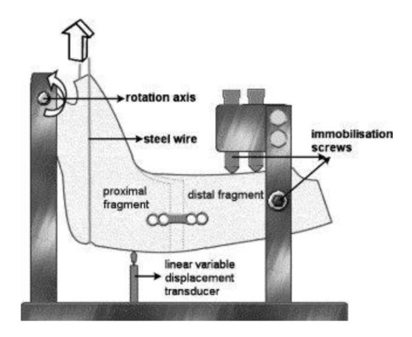
Example image for drawing modality (reproduced with permission [19]).
Figure 3.
Example image for flowchart modality (reproduced with permission [20]).
Figure 4.
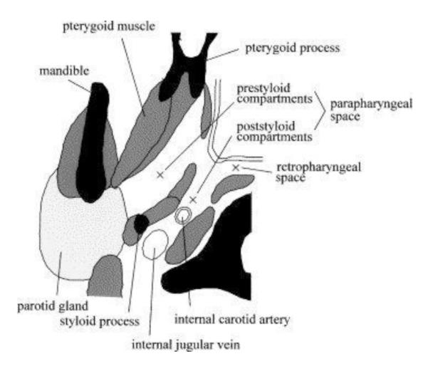
Example image for form modality (reproduced with permission [21]).
Figure 5.
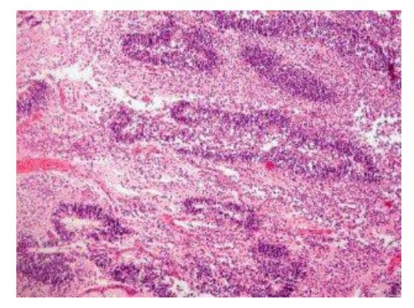
Example image for histology modality (reproduced with permission [22]).
Figure 6.
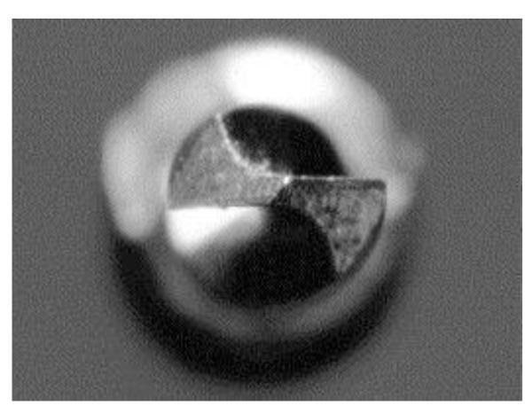
Example image for photography modality (reproduced with permission [23]).
Figure 7.

Example image for radiology modality (reproduced with permission [24]).
Figure 8.
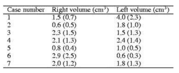
Example image for table modality (reproduced with permission [25]).
Table 8.
Average confusion matrix test results for Group 2 for δ = 1.0 from radial clustering method.
| Category\Category | 1 | 2 | 3 | 4 | 5 | 6 | 7 | 8 | 9 |
|---|---|---|---|---|---|---|---|---|---|
| 1 | 10.44 | 0.48 | 0 | 0 | 0 | 0.08 | 0 | 0 | 0 |
| 2 | 0.48 | 6.36 | 0 | 0.04 | 0 | 0.12 | 0 | 0 | 0 |
| 3 | 0.16 | 0 | 0.68 | 0 | 0 | 0 | 0.16 | 0 | 0 |
| 4 | 0.04 | 0 | 0 | 0.68 | 0 | 0 | 0 | 0.28 | 0 |
| 5 | 0 | 0 | 0 | 0 | 13 | 0 | 0 | 0 | 0 |
| 6 | 0.12 | 0.44 | 0 | 0 | 0 | 24.4 | 0 | 0 | 0.04 |
| 7 | 0.04 | 0 | 0.12 | 0.04 | 0.2 | 0.08 | 10.48 | 0 | 0.04 |
| 8 | 0 | 0 | 0 | 0.44 | 0 | 0 | 0 | 4.56 | 0 |
| 9 | 0 | 0.04 | 0 | 0 | 0.08 | 0 | 0 | 0 | 0.88 |
5. Acknowledgment
This work was supported by NLM under contract number 276200800413P and the Intramural Research Program of the National Institutes of Health (NIH), NLM, and Lister Hill National Center for Biomedical Communications (LHNCBC).
Footnotes
Publisher's Disclaimer: This is a PDF file of an unedited manuscript that has been accepted for publication. As a service to our customers we are providing this early version of the manuscript. The manuscript will undergo copyediting, typesetting, and review of the resulting proof before it is published in its final citable form. Please note that during the production process errors may be discovered which could affect the content, and all legal disclaimers that apply to the journal pertain.
6. References
- 1.Demner-Fushman D, Antani S, Thoma GR. Automatically finding images for clinical decision support. Proc. Seventh IEEE International Conference on Data Mining Workshops.2007. pp. 139–144. [Google Scholar]
- 2.Deserno TM, Antani S, Long LR. Content-based image retrieval for scientific literature access. Methods of Information in Medicine. 2009;48(4):371–80. doi: 10.3414/ME0561. [DOI] [PubMed] [Google Scholar]
- 3.Demner-Fushman D, Antani S, Simpson M, Thoma GR. Annotation and retrieval of clinically relevant images. International Journal of Medical Informatics. 2009;78:e59–e67. doi: 10.1016/j.ijmedinf.2009.05.003. [DOI] [PMC free article] [PubMed] [Google Scholar]
- 4.Hiremath PS, Pujari J. Content based image retrieval using color texture and shape features. Proc. 15th International Conference on Advanced Computing and Communications.2007. pp. 780–784. [Google Scholar]
- 5.Jalaja K, Bhagvati C, Deekshatulu BL, Pujari AK. Texture element feature characterizations for CBIR. Proc. 2005 IEEE International Geoscience and Remote Sensing Symposium.2005. pp. 733–736. [Google Scholar]
- 6.Hua Y, Xiao-Ping Z. Texture image retrieval based on a Gaussian mixture model and similarity measure using a Kullback divergence. Proc. IEEE International Conference on Multimedia and Expo.2004. pp. 1867–1870. [Google Scholar]
- 7.Patino-Escarcina RE, Costa J.A. Ferreira. The semantic clustering of images and its relation with low level color features. Proc. IEEE International Conference on Semantic Computing.2008. pp. 74–79. [Google Scholar]
- 8.Deng Y, Manjunath BS, Kenney C, Moore MS, Shin H. An efficient color representation for image retrieval. IEEE Trans Image Proc. 2007;10(1):140–147. doi: 10.1109/83.892450. [DOI] [PubMed] [Google Scholar]
- 9.Soffer A. Image categorization using texture features. Proc. Fourth International Conference on Document Analysis and Recognition.1997. pp. 233–237. [Google Scholar]
- 10.Tao D, Li X, Yuan Y, Yu N, Liu Z, Tang X. A set of novel textural features based on 3D co-occurrence matrix for content-based image retrieval. Proc. Fifth International Conference on Information Fusion.2002. pp. 1403–1407. [Google Scholar]
- 11.Sergyan S. Color histogram features based image classification in content-based image retrieval systems. Proc. 6th International Symposium on Applied Machine Intelligence and Informatics.2008. pp. 221–224. [Google Scholar]
- 12.Huihui H, Wei H, Zhigang L, Weirong C, Qingquan Q. Content-based color image retrieval via lifting scheme. Proc. International Symposium on Autonomous Decentralized Systems.2005. pp. 378–383. [Google Scholar]
- 13.Vadivel A, Majumdar AK, Sural S. Characteristics of weighted feature vector in content based image retrieval applications. Proc. IEEE Conference on Intelligent Sensing and Information Processing.2004. pp. 127–132. [Google Scholar]
- 14.Patino-Escarcina RE, Costa JAF. Content based image retrieval using a descriptors hierarchy. Proc. 7th International Conference on Hybrid Intelligent Systems.2007. pp. 228–233. [Google Scholar]
- 15.Jianhua L, Mingsheng L, Yan C. User interest model-based image retrieval technique. Proc. IEEE Conference on Automation and Logistics.2007. pp. 2265–2269. [Google Scholar]
- 16.Frigui H, Caudill J, Chamseddine B, Adballah A. Fusion of multi-modal features for efficient content-based image retrieval. Proc. IEEE International Conference on Fuzzy Systems.2008. pp. 1992–1998. [Google Scholar]
- 17.Stanley RJ, Stoecker WV, Moss RH. A basis function feature-based approach for skin lesion discrimination in dermatology dermoscopy images. Skin Research and Technology. 2008;14(4):425–435. doi: 10.1111/j.1600-0846.2008.00307.x. [DOI] [PMC free article] [PubMed] [Google Scholar]
- 18.Saka B, Petsch I, Hingst V, Hartel J. The influence of pre- and intraoperative positioning of the condyle in the centre of the articular fossa on the position of the disc in orthognathic surgery. A magnetic resonance study. British Journal of Oral and Maxillofacial Surgery. 2004;42(2):120–126. doi: 10.1016/S0266-4356(03)00236-5. [DOI] [PubMed] [Google Scholar]
- 19.Dolanmaz D, Uckan S, Isik K, Saglam H. Comparison of stability of absorbable and titanium plate and screw fixation for sagittal split ramus osteotomy. British Journal of Oral and Maxillofacial Surgery. 2004;42(2):127–132. doi: 10.1016/S0266-4356(03)00234-1. [DOI] [PubMed] [Google Scholar]
- 20.Sugar A, Bibb R, Morris C, Parkhouse J. The development of a collaborative medical modelling service: organisational and technical considerations. British Journal of Oral and Maxillofacial Surgery. 2004;42(4):323–330. doi: 10.1016/j.bjoms.2004.02.025. [DOI] [PubMed] [Google Scholar]
- 21.Umeda M, Minamikawa T, Komatsubara H, Ojima Y, Shibuya Y, Yokoo S, Komori T. En bloc resection of the primary tumour and cervical lymph nodes through the parapharyngeal space in patients with squamous cell carcinoma of the maxilla: A preliminary study. British Journal of Oral and Maxillofacial Surgery. 2005;43(1):17–22. doi: 10.1016/j.bjoms.2004.10.003. [DOI] [PubMed] [Google Scholar]
- 22.Bergé SJ, von Lindern JJ, Appel T, Braumann B, Niederhagen B. Diagnosis and management of cervical teratomas. British Journal of Oral and Maxillofacial Surgery. 2004;42(1):41–45. doi: 10.1016/s0266-4356(03)00174-8. [DOI] [PubMed] [Google Scholar]
- 23.Allan W, Williams ED, Kerawala CJ. Effects of repeated drill use on temperature of bone during preparation for osteosynthesis self-tapping screws. British Journal of Oral and Maxillofacial Surgery. 2005;43(4):314–319. doi: 10.1016/j.bjoms.2004.11.007. [DOI] [PubMed] [Google Scholar]
- 24.Ishikawa M, Mizuno T, Yamazaki Y, Satoh T, Notani K-I, Fukuda H. Migration of gutta-percha point from a root canal into the ethmoid sinus. British Journal of Oral and Maxillofacial Surgery. 2004;42(1):58–60. doi: 10.1016/s0266-4356(03)00175-x. [DOI] [PubMed] [Google Scholar]
- 25.Harrison JA, Nixon MA, Fright WR, Snape L. Use of hand-held laser scanning in the assessment of facial swelling: a preliminary study. British Journal of Oral and Maxillofacial Surgery. 2004;42(1):8–17. doi: 10.1016/s0266-4356(03)00192-x. [DOI] [PubMed] [Google Scholar]
- 26.Hain SF. Positron emission tomography in cancer of the head and neck. British Journal of Oral and Maxillofacial Surgery. 2005;43(1):1–6. doi: 10.1016/j.bjoms.2004.09.006. [DOI] [PubMed] [Google Scholar]
- 27.Bardet J-M, Lang G, Oppenheim G, Philippe A, Stoev S, Taqqu MS. Semiparametric estimation of the long-range dependence parameter: a survey. In: Doukhan P, Oppenheim G, Taqqu MS, editors. Theory and Applications of Long-Range Dependency. Birkhauser; 2003. pp. 557–577. [Google Scholar]
- 28.Piper J, Granum E. On fully automatic feature measurement for banded chromosome classification. Cytometry. 1989;10:242–255. doi: 10.1002/cyto.990100303. [DOI] [PubMed] [Google Scholar]
- 29.Haralick RM, Shapiro LG. Computer and Robot Vision. Vol. 1. Addison-Wesley Publishing Co.; New York: 1992. [Google Scholar]
- 30.Fukunaga K, Hosteler LD. The estimation of the gradient of a density function, with applications in pattern recognition. IEEE Trans Information Theory. 1975;21(1):32–40. [Google Scholar]


