Predicting Potential Placebo Effect in Drug Treated Subjects

Abstract

Non-specific responses to treatment (commonly known as placebo response) are pervasive when treating mental illness. Subjects treated with an active drug may respond in part due to non-specific aspects of the treatment, i.e, those not related to the chemical effect of the drug. To determine the extent a subject responds due to the chemical effect of a drug, one must disentangle the specific drug effect from the non-specific placebo effect. This paper presents a unique statistical model that allows for the separate prediction of a specific effect and non-specific effects in drug treated subjects. Data from a clinical trial comparing fluoxetine to a placebo for treating depression is used to illustrate this methodology.

1. Introduction

A longstanding problem in clinical practice and research is to identify and differentiate the non-specific effects of treatment from the specific effects that are due to the chemical in the drug. Non-specific response is perhaps the biggest problem in antidepressant clinical research (e.g., Womack et al., 2001), where response rates can be very high among placebo treated subjects. High response rates in the placebo arms of clinical trials for depression have led to controversies over the efficacy of drug treatments. For example, Kirsch et al. (2008) claim that the difference in response between antidepressant medication and placebo falls below accepted criteria for clinical significance except for the most severely depressed subjects and that this difference occurs due to a decreased response to non-specific effects of treatment. To clear up confusion and controversies regarding the efficacy of drug treatments in the presence of non-specific effects, statistical methods must be available to differentiate the specific from the non-specific responses in subjects treated with active drug. Such methods can also lead to improved clinical practice by allowing the identification of subjects that require the specific effect of a drug in order to improve.

The problem of identifying specific and non-specific responses is complicated because these effects are latent and not directly measured. When a subject responds to a drug treatment, we cannot measure whether s/he responded to the specific or to the non-specific effects of the treatment. An additional complication is that a subject may respond to both specific and non-specific effects and the degree of each can vary from subject to subject.

Earlier attempts to distinguish the specific drug effect from non-specific (i.e. placebo) effects were based on the use of a longitudinal “pattern analysis” (Quitkin et al., 1987a,b, 2000; Stewart et al., 1998b,a; Ross et al., 2002) where a binary pattern is generated for each subject based on weekly improvement or non-improvement throughout the trial. According to this criterion, responders to the specific drug effect had a delayed onset followed by persistence once improvement begins. A complication with this approach is that a subject may experience an immediate response to non-specific effects followed by a delayed response to the specific action of the drug and it is difficult to determine the persistence and strength of the non-specific effects in the presence of specific effects.

In a previous study, Tarpey et al. (2003) estimated functional response profiles of depressed subjects treated with phenelzine; the profile curves were partitioned using a principal point methodology (Flury, 1990, 1993). The principal point approach does not assume that these classifications correspond to real sub-populations. Instead, the partitioning based on principal points identifies a set of prototypical response profiles from a homogeneous population and subjects can be classified to the nearest prototypical principal point curve. An alternative approach would be to use a growth mixture model (e.g., Muthén and Shedden, 1999; James and Sugar, 2003; Elliott et al., 2005) based on the assumption that well-defined and distinct latent groups exist corresponding to responders to specific and non-specific effects. If subjects can experience both specific and non-specific effects and the degree of these effects can vary continuously, then the finite mixture model does not seem to be a reasonable approach. More recently Tarpey and Petkova (2008) have proposed an infinite mixture model for placebo effect, but this approach has not been generalized to longitudinal models.

In this paper, instead of attempting to partition subjects into clinically meaningful groups or assuming distinct groups exist as in a growth mixture model, a different path is taken. Given the observed response of a drug treated subject, we model the potential outcome had the subject been treated with a placebo pill instead. This approach acknowledges that a drug treated subject can respond in part due to non-specific effects and the goal is to predict this potential placebo response given the observed outcome from treatment with drug. We develop a model with components corresponding to non-specific and specific effects that can be estimated under a set of reasonable assumptions using data from clinical trials.

Section 2 presents a hypothetical experiment isolating specific and non-specific effects that serves as the underpinning for the model introduced in Section 3. The potential non-specific effect given an observed outcome from drug treatment is modeled in Section 4 along with details on estimating the parameters of the model. The model is demonstrated on data from a depression trial that compared a fluoxetine treatment to a placebo pill in Section 5. Final remarks are given in Section 6.

2. Specific and Non-Specific Effects

Consider the following thought experiment: suppose a group of subjects suffering from a particular illness and receiving no treatment are secretly observed without their knowledge. Because the subjects are not receiving any attention nor treatment, there cannot be any specific nor non-specific effects of treatment. If the population is relatively stable, the trajectories of symptoms over time will follow a flat line with random deviations due to spontaneous improvement or deterioration.

In the second scenario, suppose the group of subjects is treated with an active drug for the illness without their knowledge. For instance, the drug is secretly slipped into their morning coffee. Because the subjects have no awareness they are receiving a drug, they can only experience the specific effect of the chemical in the drug. Non-specific effects of treatment such as knowledge of taking a pill (i.e., the pill effect), expectations for improvement, and comfort from attention by clinicians will not be experienced by these subjects. Note that a non-specific effect (such as hopes for being cured) can be generated by an objective improvement due to the specific effect of the drug. Such effect, although not directly due to the chemical component in the drug, will still be present only in subjects treated with drug. Therefore, we include such possible effects in the specific effect.

In the third scenario, suppose the subjects are treated by clinicians but the pill they are given is a placebo. These subjects are lied to and told that the pill could improve their symptoms from the illness. These subjects receive active attention from clinicians and staff and have an expectation that the pill may improve their symptoms. In this scenario, responses will be due only to non-specific treatment effects.

None of the above scenarios can occur in practice. In the first scenario, the act of measuring a response involves interacting with subjects which in turn can affect the response, a problem akin to the Heisenberg Uncertainty Principle. The second scenario is unethical because patients cannot be treated without their consent. The last scenario is also unethical because it involves deliberately misleading subjects.

In reality, when subjects are given an active treatment, their responses are comprised of components from all three scenarios. If the longitudinal outcomes are modelled with mixed effects, the variability in the random effects would have a component from scenario 1 as well as a specific and non-specific components for scenarios 2 and 3.

The non-specific treatment effect is psychological, due to factors such as expectations for improvement and effect of receiving attention from clinicians. Technically, what we call a “non-specific effect” is the “non-specific effect given the specific effect is zero,” i.e., the effect observed when the subject does not receive the chemical in the drug. The “specific effect” is the combination of all effects that would not have occurred if subjects are treated with a placebo: physiological effects of the drug plus any non-specific effect that occurs from taking the drug (but would not have occurred if taking a placebo instead). Justification for such nomenclature is that when estimating drug efficacy, it is the totality of effects of the drug that do not happen on placebo that are of interest: when treating subjects, clinicians are interested in identifying those patients that would have experienced their improvements without the drug and distinguishing them from those who would not have experienced the improvements without the drug. For this reason the “specific” and “non-specific” effects in the statistical model in the next section are assumed to be independent. In Section 6 we review work on the mechanisms of placebo effect that justify the assumption of independence and elaborate further on the plausibility and the implications of this assumption.

3. Models for Drug and Placebo Treatment

In this section we develop a model for longitudinal outcomes of subjects treated with placebo and drug as a function of the unobservable specific and non-specific effects defined in the previous section, starting with the hypothetical outcome from a no-intervention treatment model. Consider the linear mixed effects model for a longitudinal outcome vector Y:

$$\mathit{\text{Y}}\hspace{0.17em}=\hspace{0.17em}\mathit{\text{X}}(\mathit{\text{β}}\hspace{0.17em}+\hspace{0.17em}\mathit{\text{b}})\hspace{0.17em}+\hspace{0.17em}\varepsilon ,$$ (1)

where X is a design matrix with q basis functions used to model the outcome Y as a function of time, β is a q × 1 vector of fixed effect coefficients and b is the q × 1 vector of random effect coefficients where b ∼ N(0, D), with unconstrained covariance matrix D. The error ε is assumed independent of b with ε ∼ N(0, σ²I). To develop placebo and drug treatment models, we partition the regression coefficients as

$$\mathit{\text{β}}\hspace{0.17em}=\hspace{0.17em}\left(\begin{array}{l}\hfill {\beta }_0\hfill \\ \hfill {\mathit{\text{β}}}_2\hfill \end{array}\right)\hspace{0.17em}\text{and}\hspace{0.17em}\mathit{\text{b}}\hspace{0.17em}=\hspace{0.17em}\left(\begin{array}{l}\hfill b_0\hfill \\ \hfill {\mathit{\text{b}}}_2\hfill \end{array}\right),$$ (2)

where β₀ and b₀ are the fixed and random effect intercepts. Because the intercept corresponds to symptom severity at baseline before treatment, the intercept β₀ should be the same for the models of no-intervention, placebo and drug treatments. In (2), β₂ and b₂ are q − 1 dimensional vectors representing features of the outcome trajectories influenced by the specific and non-specific treatment effects. For example, in the quadratic case, q = 3 and β₂ and b₂ contain the slope and curvature of the trajectories.

The mean response profile in the no-intervention model is flat and therefore β₂ = 0. In the placebo and drug treatment models, we will assume there is a 1-dimensional fixed effect direction in the coefficient space for the specific effect α_d and non-specific effect α_p. Here α_d and α_p are unit vectors in ℜ^q−1 and we assume α_d ≠ α_p. Let μ_d and μ_p denote the mean magnitude of specific and non-specific effects in directions α_d and α_p respectively. Let ${\gamma }_d^2$ and ${\gamma }_p^2$ denote the specific and non-specific subject level variability in these directions. Subject level random effects for specific and non-specific effects in these directions are denoted z_d and z_p respectively. Per the discussion in the previous section, we assume z_d and z_p are independent. More on this assumption is presented in Section 6. Additionally we assume each is standard normal. Table 1 gives the model formulations for the outcome from each of the three treatment conditions.

Table 1:

Models for data from treatment studies

Tx	Fixed effects β	Random effects b	Error
None	$\left(\begin{array}{l}\hfill \begin{array}{l}\hfill {\beta }_0\hfill \\ \hfill 0\hfill \end{array}\hfill \end{array}\right)$	$\left(\begin{array}{l}\hfill \begin{array}{l}\hfill b_{0n}\hfill \\ \hfill b_{2n}\hfill \end{array}\hfill \end{array}\right)$	${\sigma }_n^2$
Pbo	$\left(\begin{array}{l}\hfill \begin{array}{l}\hfill {\beta }_0\hfill \\ \hfill {\mu }_p{\mathit{\text{α}}}_p\hfill \end{array}\hfill \end{array}\right)$	$\left(\begin{array}{l}\hfill \begin{array}{l}\hfill b_{0p}\hfill \\ \hfill b_{2p}\hfill \end{array}\hfill \end{array}\right)\hspace{0.17em}+\hspace{0.17em}\left(\begin{array}{l}\hfill \begin{array}{l}\hfill 0\hfill \\ \hfill {\gamma }_p{z}_p{\mathit{\text{α}}}_p\hfill \end{array}\hfill \end{array}\right)$	${\sigma }_p^2$
Drug	$\left(\begin{array}{l}\hfill \begin{array}{l}\hfill {\beta }_0\hfill \\ \hfill {\mu }_p{\mathit{\text{α}}}_p\hspace{0.17em}+\hspace{0.17em}{\mu }_d{\mathit{\text{α}}}_d\hfill \end{array}\hfill \end{array}\right)$	$\left(\begin{array}{l}\hfill \begin{array}{l}\hfill {\mathbf{\text{b}}}_{0d}\hfill \\ \hfill b_{2d}\hfill \end{array}\hfill \end{array}\right)\hspace{0.17em}+\hspace{0.17em}\left(\begin{array}{l}\hfill \begin{array}{l}\hfill 0\hfill \\ \hfill {\gamma }_p{z}_p{\mathit{\text{α}}}_p\hfill \end{array}\hfill \end{array}\right)\hspace{0.17em}+\hspace{0.17em}\left(\begin{array}{l}\hfill \begin{array}{l}\hfill 0\hfill \\ \hfill {\gamma }_d{z}_d{\mathit{\text{α}}}_d\hfill \end{array}\hfill \end{array}\right)$	${\sigma }_d^2$

The 1-dimensional specific and non-specific effect models can be generalized to higher dimensions by simply allowing a larger set of basis vectors to represent each of these effects. When q is small, as in the case of quadratic profiles considered in Section 5, the 1-dimensional specific and non-specific effects are tenable assumptions. If the first principal component of the random covariance matrix from the placebo arm of a treatment study accounts for most of the variability, then the 1-dimensional non-specific model is reasonable.

The one-dimensional model for placebo effect can be motivated by the concept of allometric extension from biology (Hills, 1982; Bartoletti et al., 1999; Tarpey and Ivey, 2006). In the case of plants or animals, the allometric extension model states that one species evolved to be an “extension” of another species along a common first principal component axis. Analogous to an evolutionary force, the non-specific effects will pull the no-intervention coefficient β₂ = 0 in the direction of non-specific effects, α_p, and consequently, the non-specific variability will be primarily in the direction of α_p.

4. Potential Placebo Response in Drug Treated Subjects

For each drug treated subject we can consider the pair (Y_d, Y_p) where Y_d is the observed longitudinal outcome and Y_p is the unobserved potential outcome had the subject been treated with placebo only. In this context, Y_p represents the outcome that would be seen if, contrary to the fact (i.e., counterfactual), the subject had been treated with a placebo only (e.g. see Neyman, 1923; Rubin, 1974). Our goal is to predict the outcome Y_p given the observed outcome Y_d. The component of Y_p associated with the intercept and a pure non-specific effect is

$$\mathit{\text{X}}(\left(\begin{array}{l}\hfill \begin{array}{l}\hfill {\beta }_0\hfill \\ \hfill {\mu }_p{\mathit{\text{α}}}_p\hfill \end{array}\hfill \end{array}\right)\hspace{0.17em}+\hspace{0.17em}\left(\begin{array}{l}\hfill b_0\hfill \\ \hfill {\gamma }_p{z}_p{\mathit{\text{α}}}_p\hfill \end{array}\right)),$$ (3)

To predict a placebo response vector given the observed drug response vector, we compute

$$\text{Potential} \text{Placebo} \text{Response} (\mathbf{\text{PPR}})\hspace{0.17em}:\hspace{0.17em}=\hspace{0.17em}E[\mathit{\text{X}}(\left(\begin{array}{l}\hfill {\beta }_0\hfill \\ \hfill {\mu }_p{\mathit{\text{α}}}_p\hfill \end{array}\right)\hspace{0.17em}+\hspace{0.17em}\left(\begin{array}{l}\hfill b_0\hfill \\ \hfill {\gamma }_p{z}_p{\mathit{\text{α}}}_p)\hfill \end{array}\right)\hspace{0.17em}|{\mathit{\text{Y}}}_d],$$ (4)

This expression can be evaluated as

$$\begin{array}{lll}\text{PPR}\hfill & =\hfill & E[\mathit{\text{X}}(\left(\begin{array}{l}\hfill {\beta }_0\hfill \\ \hfill {\mu }_p{\mathit{\text{α}}}_p\hfill \end{array}\right)\hspace{0.17em}+\hspace{0.17em}\left(\begin{array}{l}\hfill b_0\hfill \\ \hfill {\gamma }_p{z}_p{\mathit{\text{α}}}_p\hfill \end{array}\right))|{\mathit{\text{Y}}}_d]\hfill \\ \hfill \hfill & =\hfill & \mathit{\text{X}}(\left(\begin{array}{l}\hfill {\beta }_0\hfill \\ \hfill {\mu }_p{\mathit{\text{α}}}_p\hfill \end{array}\right)\hspace{0.17em}+\hspace{0.17em}\left(\begin{array}{l}\hfill E[b_0|{\mathit{\text{Y}}}_d]\hfill \\ \hfill {\gamma }_p{\mathit{\text{α}}}_{p}E[z_p|{\mathit{\text{Y}}}_d]\hfill \end{array}\right))\hfill \\ \hfill \hfill & =\hfill & \mathit{\text{X}}(\left(\begin{array}{l}\hfill {\beta }_0\hfill \\ \hfill {\mu }_p{\mathit{\text{α}}}_p\hfill \end{array}\right)\hspace{0.17em}+\hspace{0.17em}\left(\begin{array}{l}\hfill E[b_0|{\mathit{\text{Y}}}_d]\hfill \\ \hfill {\gamma }_p{\mathit{\text{α}}}_p\text{cov}(z_p,{\mathit{\text{Y}}}_d){\mathbf{\text{Ψ}}}_d^{-1}({\mathit{\text{Y}}}_d\hspace{0.17em}-\hspace{0.17em}E[{\mathit{\text{Y}}}_d])\hfill \end{array}\right))\hfill \\ \hfill \hfill & =\hfill & \mathit{\text{X}}(\left(\begin{array}{l}\hfill {\beta }_0\hfill \\ \hfill {\mu }_p{\mathit{\text{α}}}_p\hfill \end{array}\right)\hspace{0.17em}+\hspace{0.17em}\left(\begin{array}{l}\hfill E[b_0|{\mathit{\text{Y}}}_d]\hfill \\ \hfill {\gamma }_p{\mathit{\text{α}}}_p(E[z_p{b}_0],\hspace{0.17em}{\gamma }_p{\mathit{\text{α}}}_p^{\prime })\hspace{0.17em}{\mathit{\text{X}}}^{\prime }{\mathbf{\text{Ψ}}}_d^{-1}({\mathit{\text{Y}}}_d\hspace{0.17em}-\hspace{0.17em}\mathit{\text{X}}{\mathit{\text{β}}}_d)\hfill \end{array}\right)),\hfill \end{array}$$ (5)

where Ψ_d = cov(Y_d), β_d is the vector of fixed effect regression coefficients from the drug arm, and we have assumed all random quantities are jointly normal so that the conditional expectation will be linear.

The potential placebo response in (5) can be estimated by fitting a standard linear mixed effects model via maximum likelihood to each arm of a placebo - controlled clinical trial. Estimates of the parameters α_p, γ_pβ₀, β_d, and Ψ_d can be obtained directly from the fitted linear mixed effects model for the placebo and drug arms. Let β̂_2p denote the estimated fixed effect coefficients for placebo treated subjects (not including the intercept term). Then μ_p and the unit vector α_p can be estimated by

$${\widehat{\mathit{\text{α}}}}_p\hspace{0.17em}=\hspace{0.17em}{\widehat{\mathit{\text{β}}}}_{2p}/\left|\right|{\widehat{\mathit{\text{β}}}}_{2p}\hspace{0.17em}\text{and}\hspace{0.17em}{\widehat{\mu }}_p\hspace{0.17em}=\hspace{0.17em}\pm \left|\right|{\widehat{\mathit{\text{β}}}}_{2p}\left|\right|$$ (6)

and the sign of μ̂_p is taken to be consistent with the placebo effect direction (i.e. so that β̂_2p = μ̂_pα̂_p). Let β_2d denote the vector of fixed effects for drug treated subjects (not including the intercept). The drug effect direction α_d, can be estimated by subtracting off the placebo effect and normalizing:

$${\widehat{\mathit{\text{α}}}}_d\hspace{0.17em}=\hspace{0.17em}\frac{{\widehat{\mathit{\text{β}}}}_{2d}\hspace{0.17em}-\hspace{0.17em}{\widehat{\mu }}_p{\widehat{\mathit{\text{α}}}}_p}{\left|\right|{\widehat{\mathit{\text{β}}}}_{2d}\hspace{0.17em}-\hspace{0.17em}{\widehat{\mu }}_p{\widehat{\mathit{\text{α}}}}_p\left|\right|}\hspace{0.17em}\text{and}\hspace{0.17em}{\widehat{\mu }}_d\hspace{0.17em}=\hspace{0.17em}\pm \left|\right|{\widehat{\mathit{\text{β}}}}_{2d}\hspace{0.17em}-\hspace{0.17em}{\widehat{\mu }}_p{\widehat{\mathit{\text{α}}}}_p\left|\right|,$$ (7)

where again the sign of μ̂_d is taken consistent with the drug effect direction.

Because the non-specific variability in the model is in the direction of α_p, we can estimate the non-specific variance ${\gamma }_p^2$ as

$${\widehat{\gamma }}_p^2={\widehat{\mathit{\text{α}}}}_p^{\prime }{\widehat{\mathit{\text{D}}}}_{2p}{\widehat{\mathit{\text{α}}}}_p,$$ (8)

where D̂_2p is the estimated random effect covariance matrix from the placebo arm for all terms except the intercept. Alternatively, the random effect covariance matrix from the drug arm D̂_2d could be used instead of D̂_2p in (8) to estimate the non-specific effect variability

$${\tilde{\gamma }}_p^2\hspace{0.17em}=\hspace{0.17em}{\widehat{\mathit{\text{α}}}}_p^{\prime }{\widehat{\mathit{\text{D}}}}_{2d}{\widehat{\mathit{\text{α}}}}_p.$$ (9)

However, ${\tilde{\gamma }}_p^2$ could include some specific effect variability making it larger than ${\widehat{\gamma }}_p^2$. In fact, in the example below, ${\tilde{\gamma }}_p^2\hspace{0.17em}>\hspace{0.17em}{\widehat{\gamma }}_p^2$. If it turns out that ${\tilde{\gamma }}_p^2\hspace{0.17em}<\hspace{0.17em}{\widehat{\gamma }}_p^2$ for a given data set, then this could indicate a problem with the model specification, such as, for example, the assumption of independence of the specific and non-specific random effects.

The best linear unbiased predictor (BLUP) of b₀ from the placebo arm will be used for E[b₀|Y_d] in (5). Finally, if a subject’s intercept is independent of the degree of the subject’s non-specific response, then E[z_pb₀] = 0. We shall assume this is a good approximation in our estimation. Justification for this assumption is given in the example of Section 5.

5. Example: Non-Specific Response in an Antidepressant Study

The potential placebo response model developed above is now applied to data from a clinical trial conducted to test the antidepressant medication fluoxetine. We will examine data from the placebo arm and also 20 and 40 mg fluoxetine arms. The randomization to placebo, 20 mg and 40 mg of the drug was 1 : 2 : 2. There was a 60 mg fluoxetine arm, but 20% of subjects dropped out before week 2 and less than 50% completed the 6 week of treatment, possibly due to intolerability of the high dose of the drug. Because the focus here is not on issues pertaining to dropout and missing data, we will confine out attention to the 20 and 40 mg arms of the study. The study recorded the subjects’ Hamilton Depression (HAM-D) scores at baseline (week 0) and for six consecutive weeks. Lower scores on the HAM-D correspond to lower levels of depression. We used quadratic functions of time (t in weeks)

$$y\hspace{0.17em}=\hspace{0.17em}{\beta }_0\hspace{0.17em}+\hspace{0.17em}{\beta }_{1}t\hspace{0.17em}+\hspace{0.17em}{\beta }_2{t}^2,$$ (10)

to model the longitudinal outcome and normal theory maximum likelihood for estimation. The software R (R Development Core Team, 2003) was used to analyze the data.

The results below will be presented using orthogonal polynomials. One reason for this is that the slope of the linear term using orthogonal polynomials equals the average tangent slope of the parabola (Tarpey, 2003) which is a measure of overall improvement throughout the trial, whereas β₁ in (10) measures the rate of improvement at baseline only. Further motivation for the use of orthogonal polynomials is given below. We will call the coefficient of the linear polynomial using orthogonal polynomials average slope.

5.1. Fitting the Model

For illustrative purposes, most of the results reported here will be using the placebo and 20 mg fluoxetine arms. Quadratic polynomial mixed effect models were fit to the placebo and drug arms for subjects with at least 3 visits (n = 98 for placebo and n = 196, and 192 for the 20 and 40 mg fluoxetine treatment arms respectively).

From the placebo arm, based on (6) the estimated non-specific effect direction is α̂_p = (−0.994, 0.111)^′ with μ̂_p = 2.834. The estimated random effect covariance matrix for the average slope and concavity is

$${\widehat{D}}_{2p}\hspace{0.17em}=\hspace{0.17em}\left(\begin{array}{ll}\hfill 6.007\hfill & \hfill -0.748\hfill \\ \hfill -0.748\hfill & \hfill 0.108\hfill \end{array}\right)\hspace{0.17em}.$$

The first eigenvector of this matrix is (−0.992, 0.124)^′ which matches closely α̂_p. The first eigenvector of this matrix accounts for 99.8% of the total random effect variability of the slope and concavity in the placebo arm. Thus, it appears that the non-specific treatment effect explains almost all of the random effect variability seen in the average slopes and concavities in the placebo arm. Additionally, the distribution of slopes and concavities for the placebo treated groups is consistent with the allometric extension idea mentioned in the previous section, because the primary direction of the random effect variability coincides with the direction of the non-specific treatment effect μ_pα_p. These results support the one-dimensional non-specific effect assumption on which the model is based.

The estimated variance component for the non-specific effect is ${\widehat{\gamma }}_p^2\hspace{0.17em}=\hspace{0.17em}6.099$, using (8). The estimated correlations between the random intercept b₀ and the random slope and concavity are estimated to be −0.0743 and −0.1026 respectively, which are quite small and provide a basis for the approximation of E[b₀z_p] ≈ 0. The total random effect variability, as measured by the trace of the estimated random effect covariance matrices, is 17.47 for the placebo arm, and 19.75 and 20.11 for the 20 and 40 mg fluoxetine arms respectively. The higher variability in the drug arms can be attributed to the specific drug effect variability that is not present in the placebo arm. It is interesting to note that in the 20 mg fluoxetine arm, the non-specific effect accounts for a very large amount of the random effect variability compared to the specific effect according to the proposed model. Because a non-specific effect corresponds to complex psychological factors and expectations, a large degree of non-specific response variability may be expected compared to a the variability due to a fixed dose (20 mg) of fluoxetine. Finally, from (7) the estimated mean specific drug effect parameters for fluoxetine (20 mg) treated subjects are α^_d = (0.3841, −0.9233)^′ and μ̂_d = 0.0862.

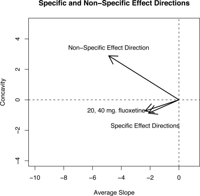
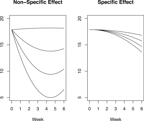
Figure 1 shows the estimated directions and magnitudes of the non-specific effect μ̂_pα̂_p and specific 20 and 40 mg effect μ̂_dα̂_d in the coefficient space of the orthogonal basis functions. Smaller values of the average slope correspond to lower HAM-D scores and hence a greater degree of improvement over the 6-week trial. The non-specific and specific effect directions point towards lower average slopes indicating that specific and non-specific effects lead to improvement in mood as expected. However, note that the non-specific effect direction corresponds to parabolas that are concave up whereas the specific effects are concave down. This confirms the empirical observations of psychiatrists who expect slow onset and persistent specific effect of antidepressant drugs, consistent with a concave down shape. Figure 2 shows parabolas representing an uncontaminated non-specific effect (left panel) and an uncontaminated specific effect (right panel) estimated from the 20 mg arm. The average slope and concavity of the parabolas shown in Figure 2 were taken along the non-specific and specific effect directions shown in Figure 1. The non-specific effect parabolas show an immediate improvement from baseline (week 0) and, depending on the strength of the non-specific effect, a deterioration in mood is seen later in the trial as the parabolas begin to bend upwards. On the other hand, the specific effect parabolas in the right panel of Figure 2 show a delayed but steady improvement. The top parabola in the right panel of Figure 2 is almost completely flat which is indicative of no specific effect.

Figure 1:

The directions of the non-specific effect μ_pα_p and the specific effect μ_dα_d for the two dose arms in the coefficient space using the orthogonal polynomials.

Figure 2:

Left panel: Non-specific effect parabolas computed using parabola coefficients obtained along the non-specific effect direction α̂_p. Right panel: Specific effect parabolas computed using parabola coefficients obtained along the specific effect direction α̂_d in the coefficient space.

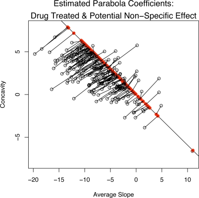
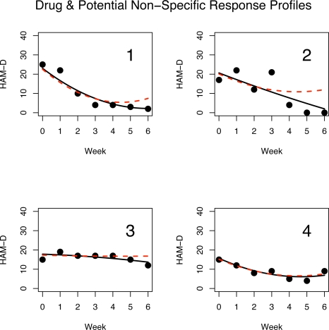
The potential non-specific response for subjects treated with drug (20 mg) is shown in Figure 3. It plots the estimated average slopes and concavities (fixed effect plus the best linear unbiased predictor or BLUP). Each coefficient is connected (via a line segment) to its projection onto the non-specific effect direction α̂_p based on the PPR given by (5). Note that the projections onto the placebo effect direction line are not necessarily orthogonal projections. Thus, Figure 3 shows the estimated parabola coefficients from the observed outcomes of subjects in the 20 mg drug arm along with the coefficients for the corresponding predicted PPR, i.e., their outcome had they been treated with placebo. Figure 4 shows the HAM-D scores and the estimated quadratic response profile (solid curve) for four subjects in the fluoxetine 20 mg arm of the trial. The four chosen examples are representative of what is seen in the full sample. The dashed curve is the predicted PPR curve based on (5). In each of the four panels of Figure 4, the estimated drug response profile overlaps with the PPR profile in the first few weeks of the trial as might be expected since SSRI drugs like fluoxetine may have little effects during the first weeks, but the non-specific treatment effect will be present in both placebo and drug treated subjects. The observed outcome curve in panel 1 shows a strong improvement at the beginning of the trial before levelling off. However, the PPR curve bends upwards towards the end of the trial indicating that this subject’s mood would have deteriorated towards the end of the six weeks if treated with a placebo instead of the active drug. Panel 2 is similar to panel 1 except that observed outcome curve appears nearly linear showing a constant rate of improvement but the PPR curve again bends upwards towards the end of the trial. Based on the proposed model, the subjects in panels 1 and 2 clearly benefit from the specific effects of the drug. The observed outcome parabola in panel 3 is concave down and shows a slow degree of improvement over the six week trial. The subject in panel 3 appears to have experienced almost no non-specific treatment effect and a small degree of a delayed specific effect. In panel 4, the observed outcome and PPR profiles almost completely overlap indicating that this subject experienced very little specific treatment effect and the outcome is almost completely due to a non-specific effect. The results in Figure 4 indicate that the fluoxetine treatment tends to maintain the positive initial non-specific effect over time and that the mood of many subjects will begin to deteriorate if treated with a placebo pill only.

Figure 3:

A plot of the estimated average slope and concavity coefficients (fixed effect plus BLUP) for drug treated subjects and the corresponding projection onto the non-specific effect direction. Note that the projections are not necessarily orthogonal projections onto the non-specific effect direction line.

Figure 4:

Weekly HAM-D outcomes for 4 drug treated subjects. The solid parabola is the estimated quadratic response profile. The dashed curve is the corresponding potential non-specific response profile using an estimate of (5).

5.2. Identifying Non-Specific Responders Among Drug Treated Subjects

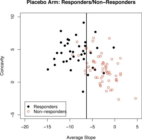
Next, we use PPR for drug treated subjects to answer the following question: which drug treated subjects are non-specific responders. That is, we want to identify subjects treated with the active drug that would have responded if treated with a placebo instead. In other words, the goal is to determine which subjects would get better by a placebo effect alone. In the fluoxetine study, the subjects in each arm were rated according to a clinician’s global impression (CGI) of improvement which is a likert scale (1 = very much improved, 2 = much improved, 3 = minimally improved, 4 = not improved, 5 = minimally worse, 6 = much worse, 7 = very much worse). Subjects who receive a CGI rating of 1 or 2 are classified as treatment responders. Defining a binary outcome variable as 0 for non-responder and 1 for a responder according to the CGI criterion, we can perform a logistic regression to determine a classification boundary for responders and non-responders. In particular, using the estimated regression coefficients (fixed effects + BLUPS) from the placebo arm as predictors, we model subjects’ response status as a function of their estimated intercept, slope, and concavity; only the average slope coefficient was statistically significant in the logistic regression. The result is a simple discriminant boundary, a vertical line between responders and non-responders in terms of a cutoff point of the average slope. The estimated cutoff is −6.295; we call this the “Placebo-group average slope discriminant” criterion (PGASD). Note that if we had not used the orthogonal polynomial basis, the boundary would be defined in terms of both the slope and concavity.

Figure 5 shows the vertical discriminant boundary line based on PGASD criterion for subjects in the placebo group. The solid circles correspond to responders (based on the CGI criterion) and the open circles correspond to non-responders. Of the n = 98 placebo treated subjects seen in Figure 5, 37.8% (37/98) were rated as responders on the CGI scale. Using the PGASD criterion, 36.7% (36/98) of the placebo treated subjects were classified as responders.

Figure 5:

A plot of estimated average slope and concavity coefficients for placebo treated responders (solid circles) and non-responders (open circles). The vertical line is the placebo-group average slope discriminant criterion (PGASD) boundary between responders and non-responders.

Table 2 shows the percentage of subjects classified as responders based on (1) their CGI criterion, (2) PGASD criterion applied to the BLUP estimates from the model for the observed outcome, and (3) PGASD criterion applied to the PPR estimates. For example, 57.1% (112/196) of subjects treated with 20 mg fluoxetine were rated as responders based on the CGI. A slightly larger percentage (59.2%) were classified as responders according to the average slope discriminant criterion. That is, 59.2% of the 20 mg fluoxetine subjects had a predicted average slope below the cutoff of −6.295.

Table 2:

Percentage of Responders in each arm

Dose	CGI	Placebo Group Average Slope Discriminant (PGASD) Criterion
		Observed	PPR
Placebo	37.8%	35.7%	35.7%
20 mg	57.1%	59.2%	38.3%
40 mg	58.9%	57.8%	40.1%

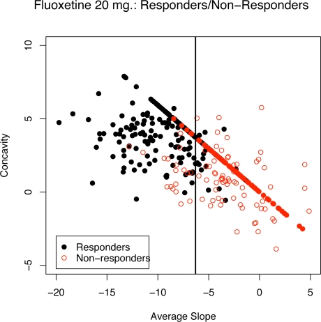
Recall that a key question is which drug treated subjects would have responded due to non-specific effects? To answer this question, we can estimate the PPR from (5) for a drug treated subject and observe if his/her average PPR slope falls below the cutoff. The last column of Table 1 gives the percentage of drug treated subjects that would have been classified as responders even if they have been treated with a placebo. Thus, 38.3% of the 20 mg fluoxetine treated subjects would have been rated as responders had they been treated only with a placebo. Figure 6 shows a plot of the estimated average slope and concavity coefficients for fluoxetine (20 mg) treated subjects where the solid circles correspond to responders (based on CGI) and the open circles correspond to non-responders. Also shown are the projections of the coefficients onto the non-specific effect direction. The vertical line is the PGASD boundary. The classification boundaries that result when fitting a logistic regression model to responders/non-responders from 20 mg and 40 mg fluoxetine groups were almost identical to the average slope discriminant boundary obtained from the placebo treated group shown in Figure 6, i.e. D₂₀GASD and D₄₀GASD criteria were very similar to PGASD.

Figure 6:

A plot of estimated average slope and concavity coefficients for fluoxetine (20 mg) treated responders (solid points) and non-responders (open points). The vertical line is the placebo-group average slope discriminant (PGASD) criterion boundary.

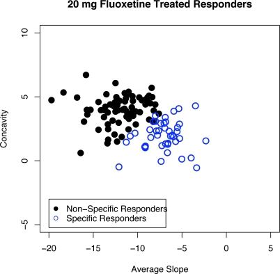
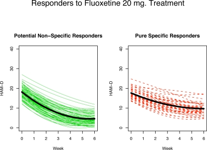
Figure 7 and Figure 8 show 20 mg fluoxetine treated responders broken down into two groups: non-specific responders, those that would have responded even if treated with a placebo (solid circles in Figure 7 and left panel of Figure 8) and specific responders, those that would not have responded if treated with placebo alone but do respond when treated with the active drug (open circles in Figure 7 and right panel of Figure 8). Figure 8 shows the estimated response profiles and the thick curve in each panel is the mean curve for each group. The non-specific responders (left panel) show a fairly strong initial decline in HAM-D followed by a levelling out towards the end of the 6-week period. The specific only responders on the other hand (right panel) show an even and fairly constant rate of improvement throughout the trial.

Figure 7:

Average slope and concavity points for the 57.1% of fluoxetine (20 mg) treated subjects who were responders based on CGI. The solid points correspond to subjects who would have responded if treated with a placebo, the “non-specific responders”, and the open circles correspond to the specific only responders.

Figure 8:

Estimated profiles for fluoxetine (20 mg) treated CGI-rated responders. Left panel: non-specific responders. Right panel: PPR non-responders. The solid curve in each panel is the mean curve for each group.

It is important to note that although the non-specific responders in the active drug groups would have responded if treated with a placebo, many of these subjects experience an enhanced outcome due to the active drug. In Tarpey et al. (2003), these subjects were labelled as mixture effects responders, subjects who respond due to a combination of a specific effect and a non-specific effect. In fact, the average slope for placebo treated responders is −8.5 whereas the average slope for non-specific responders in the fluoxetine (20 mg) arm is −12.0 and a simple t-test comparing the average slopes yields a significant difference (t = −6.013, p < 0.0001, df = 104). In other words, the coefficient distribution for non-specific responders among the drug treated subjects is shifted significantly towards greater improvement than the responders among the placebo treated subjects. This indicates that although the drug treated non-specific responders would have responded due only to non-specific effect, many of those subjects also enjoy additional benefit from a drug effect.

5.3. Parametric Bootstrap Simulation

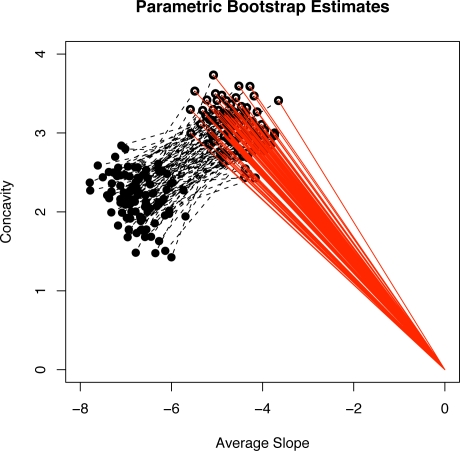
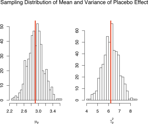
A parametric bootstrap simulation was conducted to assess the uncertainty in the parameter estimates. 500 placebo and fluoxetine 20 mg data sets were simulated where the parameters used in the simulation model were equal to the estimated parameters from the actual data. Figure 9 shows a plot of 100 of the 500 estimated placebo effect direction vectors μ̂_pα̂_p in the coordinate system of the average slope and concavity. A 95% bootstrap confidence interval for the polar angle θ defining α_p = (cos(θ), sin(θ))^′ is (131.3⁰, 145.3⁰). Figure 9 also shows line segments (the dashed segments) connecting the estimated slope and concavity for placebo treated subjects to the estimated slope and concavity for drug treated subjects from the same simulated sample. The distribution of these dashed segments indicate the variability in estimating the polar angle defining α_d is substantially higher than the variability in estimating the polar angle for the placebo effect direction. The reason for this is that the estimated drug effect direction α̂_d is defined as a difference between the estimated fixed effects for drug treated subjects minus the estimated placebo effect direction in (7) and thus has an additional source of variation that is not present in estimating the placebo effect direction. However, based on the assumptions we have made, μ̂_d and α̂_d are not required for computing the predicted potential placebo response (5). Figure 10 shows the parametric bootstrap histograms for the estimated mean placebo effect μ̂_p and variance of the placebo effect γ̂_p. The vertical line in each histogram shows the estimate from the original data. Both histograms indicate that the estimators of μ_p and ${\gamma }_p^2$ are approximately unbiased and normally distributed.

Figure 9:

Plot of placebo direction vectors μ̂_pα̂_p (solid lines) and their connections (dashed lines) to the estimated average slopes and concavities for the drug group from 100 simulated data sets.

Figure 10:

Histograms of the 500 estimated mean placebo effects μ̂_p and estimated placebo variances ${\widehat{\gamma }}_p^2$. The vertical lines represent the parameter estimates from the raw data.

6. Discussion

Subjects in depression treatment studies are classified as responders or non-responders. This paper contributes to the long standing problem of classifying responders as either specific or non-specific responders to the antidepressant treatment. Such classifications are somewhat artificial. According to the model proposed in this paper, the latent specific and non-specific effects are represented by continuous random effects. Accordingly, subjects can experience both specific and non-specific treatment effects and the strength of these effects can vary continuously. Therefore, if a subject is classified as a specific responder according to the proposed model, this does not necessarily mean the subject did not experience any non-specific effects. What it does mean is that if the subject did experience a non-specific effect, it was not strong enough in of itself to make the subject a responder. In other words, the subject needs the drug to meet the criterion for responder.

This paper has focused on isolating non-specific treatment effects in drug treated subjects, a recurrent problem in clinical research. An attempt to solve this problem is the introduction of a washout period at the beginning of a trial where study participants are given placebo, which is a common practice, especially in depression research. The hope is that non-specific responders to treatment will be eliminated or their number reduced. A problem with this approach is that the subjects who are eliminated due to an initial non-specific response could experience a response due to specific effects later once the drug has a chance to take effect. The model proposed in this paper also allows for the estimation of specific drug effects by filtering out the non-specific effect by projecting a subject’s response onto the specific effect direction.

The PPR model introduced in this paper is based on a few assumptions. The two most important assumptions perhaps are that the specific and non-specific effects denoted by z_p and z_d are independent and are 1-dimensional. The one-dimensional drug and placebo effect assumptions can be regarded as a principal component approximation to a higher dimensional distribution and can be relaxed when using higher dimensional bases for fitting the longitudinal outcomes. The results of the fluoxetine trial in Section 5 supports the one-dimensional placebo effect model. The assumption of independence deserves some elaboration.

According to all theories about the mechanisms of placebo effect we are aware of, if the specific and non-specific effects in drug-treated subjects are associated, it is the specific effects that would influence the non-specific effect and the potential association can only be is positive: presence and increase in specific effect should increase the non-specific effects (see Kirsch (1985, 1990); Orne (1969); Wickamasekera (1980); Ader and Cohen (1991)). While theories about placebo effects are concerned with the mechanisms of improvement due to non-specific aspects of the treatment, a major question in clinical practice is the efficacy of a drug and (in depression treatment), whether or not a patient who was treated and improved did so due to specific or non-specific effects, i.e. does s/he need the drug or not. For the purposes of addressing these pragmatic questions, here we use as a definition of specific effect, the outcome that would not have happened had the subject been treated with placebo only. As explained in Section 2, this includes the true specific effect of the drug plus any non-specific effects that resulted from a true specific effect including side effects from the drug. Under this pragmatic definition, if presence of specific effect enhances the non-specific effect, the enhancement is considered a part of the specific effect. Hence, for the purposes of addressing the pragmatic question, the specific and non-specific effects are additive and independent. Consequently, the variability in a drug-treated group is considered to be a sum of the variances of z_p and z_d and cov(z_p, Y_d) reduces to (E[z_pb₀], γ_pα_p) in (5). Note, that in the example presented in Section 5.1, the variation of the random effects in the placebo group is only minimally smaller than the variation in the two drug arms. Because the variance in a drug arm is a sum of the variation of specific and non-specific effects, this indicates that the specific effects have much smaller variability compared to the variability in the non-specific effects. This can be expected since the specific effect is physiological, resulting from a (deterministic) chemical process, whereas the non-specific effect encompasses all other sources of variability between subjects including psychological factors such as patient’s expectations and the impact of clinicians’ attention on them.

Although it is not possible to estimate the association between specific and non-specific random effects, one can evaluate the boundaries, between which the inferences of interest can change if these effects are correlated. An association between specific and non-specific effects, which would be positive as per the discussion above, would imply that the specific effect variation is even smaller. For example, from Section 5.1, the trace of the variance-covariance matrix for the random effect in the placebo arm is 17.47 and for the 20 mg drug arm it is 19.75; thus the variance of the specific effects alone can not be higher that (19.74 − 17.47) = 2.28 which is 11.2% of the total random effect variability in the drug arm. If the correlation between specific and non-specific effects increases from zero to one, the proportion of specific effect variability in the drug arm drops rapidly towards zero with a proportion of 0.004 when the correlation is 1. Thus, positive correlations between specific and non-specific in essence imply that the specific effect is the same across all subjects and all random variation is due to the variation of non-specific effects between subjects. This is an interesting result of itself. Section 5.2 identifies those responders to drug treatment who would not have been responders if treated with placebo, called specific responders. By performing the analysis assuming different correlations between specific and non-specific effect, one can identify subjects who remain in the category of specific responders for all values of the correlation. Of course, pragmatically, this would not be a correct way of finding the responders to specific drug effect – such approach would be qualifying as non-specific responders on drug individuals who would not have been responders on placebo and thus, according to the pragmatic definition, would not be non-specific responders.

Of note, the proposed model allows for the specific effect to be negative, i.e., the PPR to be better than the observed outcome on drug, see Figure 3 where the points above the projection line corresponds to a worse outcome on drug than on placebo. One explanation for such occurrence is that a fraction of subjects could have had an adverse reaction to the drug which might translate to a poorer mood than if they had received a placebo instead. If this explanation is not reasonable, then a modification of the model could be considered by constraining the pure drug effect z_d to be positive in which case the distribution for the pure drug effect would likely be skewed in the direction of improvement. This constraint would complicate parameter estimation considerably because standard normal theory mixed effect models could no longer be used and the linear conditional expectation may no longer hold.

References

- Ader R, Cohen N. The influence of conditioning on immune responses. In: Ader R, Felten DL, Cohen N, editors. Psychoneuroimmunology. Academic Press; San Diego: 1991. pp. 611–646. [Google Scholar]
- Bartoletti S, Flury B, Nel D. Allometric extension. Biometrika. 1999;55:1210–1214. doi: 10.1111/j.0006-341x.1999.01210.x. [DOI] [PubMed] [Google Scholar]
- Elliott MR, Gallo JJ, Ten Have TR, Bogner HR, Katz IR. Using a bayesian latent growth curve model to identify trajectories of positive affect and negative events following myocardial infarction. Biostatistics. 2005;6:119143. doi: 10.1093/biostatistics/kxh022. [DOI] [PMC free article] [PubMed] [Google Scholar]
- Flury B. Principal points. Biometrika. 1990;77:33–41. doi: 10.1093/biomet/77.1.33. [DOI] [Google Scholar]
- Flury B. Estimation of principal points. Applied Statistics. 1993;42:139–151. doi: 10.2307/2347416. [DOI] [Google Scholar]
- Hills M. Allometry. In: Kotz S, Read CB, Banks DL, editors. Encyclopedia of Statistical Sciences. Vol. 1. Wiley; 1982. pp. 48–54. [Google Scholar]
- James G, Sugar C. Clustering for sparsely sampled functional data. Journal of the American Statistical Association. 2003;98:397–408. doi: 10.1198/016214503000189. [DOI] [Google Scholar]
- Kirsch I. Response expectancy as a determinant of experience and behavior. American Psychologist. 1985;40:1189–1202. doi: 10.1037/0003-066X.40.11.1189. [DOI] [Google Scholar]
- Kirsch I. Changing Expectations: A Key to Effective Psychotherapy. Brooks/Cole; Pacific Grove, California: 1990. [Google Scholar]
- Kirsch I, Deacon BJ, Huedo-Medina TB, Scoboria A, Moore TJ, Johnson BT. Initial severity and antidepressant benefits: A meta-analysis of data submitted to the food and drug administration. PLOS Medicine. 2008;5:E45. doi: 10.1371/journal.pmed.0050045.. [DOI] [PMC free article] [PubMed] [Google Scholar]
- Muthén B, Shedden K. Finite mixture modeling with mixture outcomes using the EM algorithm. Biometrics. 1999;55:463–469. doi: 10.1111/j.0006-341X.1999.00463.x. [DOI] [PubMed] [Google Scholar]
- Neyman J. On the application of probability theory to agricultural experiments: Essays on principles, section 9. translated from the Polish and edited by D. M. dabrowska and T. P. Speed. Statistical Science. 1923;1990;5:465. [Google Scholar]
- Orne MT. Demand characteristics and the concept of quasi-controls. In: Rosental R, Rosnow RL, editors. Artifact in Behavioral Research. Academic Press; New York: 1969. pp. 142–179. [Google Scholar]
- Quitkin FM, Rabkin JD, Markowitz JM, Stewart JW, McGrath PJ, Harrison W. Use of pattern analysis to identify true drug response. Archives of General Psychiatry. 1987a;44:259–264. doi: 10.1001/archpsyc.1987.01800150071009. [DOI] [PubMed] [Google Scholar]
- Quitkin FM, Rabkin JD, Ross D, Stewart JW. Identification of true drug response to antidepressants: Use of pattern analysis. Archives of General Psychiatry. 1987b;41:782–786. doi: 10.1001/archpsyc.1984.01790190056007. [DOI] [PubMed] [Google Scholar]
- Quitkin FM, Rabkin JG, Davis GJ, Klein DF. Validity of clinical trials of antidepressants. The American Journal of Psychiatry. 2000;157:327–337. doi: 10.1176/appi.ajp.157.3.327. [DOI] [PubMed] [Google Scholar]
- R Development Core Team. R: A language and environment for statistical computing. R Foundation for Statistical Computing; Vienna, Austria: 2003. [Google Scholar]
- Ross DC, Quitkin FM, Klein DF. A typological model for estimation of drug and placebo effects in depression. Journal of Clinical Psyhopharmacology. 2002;22:414–418. doi: 10.1097/00004714-200208000-00013. [DOI] [PubMed] [Google Scholar]
- Rubin DB. Estimating causal effects of treatments in randomized and non-randomized studies. Journal of Educational Psychology. 1974;66:688–701. doi: 10.1037/h0037350. [DOI] [Google Scholar]
- Stewart JW, Quitkin FM, McGrath PJ, Amsterdam J, Fava M, Fawcett J, Reimherr F, Rosenbaum J, Beasley C, Roback P. Use of pattern analysis to predict differential relapse of remitted patients with major depression during 1 year of treatment with fluoxetine or placebo. Archives of General Psychiatry. 1998a;55:334–343. doi: 10.1001/archpsyc.55.4.334. [DOI] [PubMed] [Google Scholar]
- Stewart JW, Quitkin FM, McGrath PJ, Amsterdam J, Fava M, Fawcett J, Reimherr F, Rosenbaum J, Beasley C, Roback P. Use of pattern analysis to predict differrential relapse of remitted patients with major depression during 1 year of treatment with fluoxetine or placebo. Archives of General Psychiatry. 1998b;55:334–343. doi: 10.1001/archpsyc.55.4.334. [DOI] [PubMed] [Google Scholar]
- Tarpey T. Estimating the average slope. Journal of Applied Statistics. 2003;30:389–395. doi: 10.1080/0266476032000035412a. [DOI] [Google Scholar]
- Tarpey T, Ivey CT. Allometric extension for multivariate regression models. Journal of Data Science. 2006;4 [Google Scholar]
- Tarpey T, Petkova E. Latent regression analysis. Statistical Modelling. 2008. To appear. [DOI] [PMC free article] [PubMed]
- Tarpey T, Petkova E, Ogden RT. Profiling placebo responders by self-consistent partitions of functional data. Journal of the American Statistical Association. 2003;98:850–858. doi: 10.1198/016214503000000783. [DOI] [Google Scholar]
- Wickamasekera I. A conditioning response model of the placebo effect: Predictions from the model. Biofeedback and Self-Regulation. 1980;5:5–18. doi: 10.1007/BF00999060. [DOI] [PubMed] [Google Scholar]
- Womack T, Potthoff J, Udell C. Placebo response in clinical trials. Applied Clinical Trials. 2001;10:32–37. [Google Scholar]