Abstract
With recent advances in mass spectrometry (MS) technologies, it is now possible to study protein profiles over a wide range of molecular weights in small biological specimens. However, MS spectra are usually not aligned or synchronized between samples. To ensure the consistency of the subsequent analysis, spectrum alignment is necessary to align the spectra such that the same biological entity would show up at the same m/z value for different samples. Although a variety of alignment algorithms have been proposed in the past, most of them are developed based on chromatographic data and do not address some of the unique characteristics of the serum or other body fluid MS data. In this work, we propose a self-calibrated warping (SCW) algorithm to address some of the challenges associated with serum MS data alignment. In addition, we compare the proposed algorithm with five existing representative alignment methods using a clinical surface enhanced laser desorption/ionization time-of-flight mass spectrometry (SELDI-TOF-MS) data set.
Keywords: mass spectrometry, alignment, warping, peak detection, feature extraction, data preprocessing, proteomics
Introduction
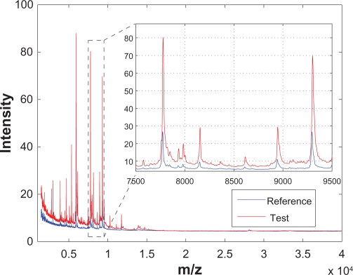
In the last few decades, various advanced high-throughput analytical instruments, such as chromatography, mass spectrometry (MS), nuclear magnetic resonance (NMR) spectroscopy, and Raman spectroscopy, have been applied to biological, biomedical and life-science research. Preprocessing of the chromatographic and spectral data generated from these instruments has been an important aspect of research to ensure consistent subsequent analyses. This is because for the chromatographic or spectral data, the locations of different peaks in a chromatogram or spectrum represent different chemical or biological entities, while the magnitudes (eg, areas or heights) of different peaks represent the relative abundance of these entities. Therefore, in order to extract chemically or biologically meaningful information from a group of samples, it is desirable that different chromatograms or spectra have the same baseline, and the peaks corresponding to the same entity show up at the same location for different spectra. In reality, however, different chromatograms or spectra obtained from different samples are usually not aligned and have different baselines. These characteristics are illustrated in Figure 1 using two spectra from a clinical SELDI-TOF-MS prostate cancer data set.1–3 Figure 1 shows two spectra generated from two different sample serums and the inset zooms in to show a segment of the both spectra. It can be seen that the spectra are noisy, especially among the small peaks that are close to the baseline; in addition, the two spectra have different baselines; and finally, the two spectra are not aligned—the peaks corresponding to the same bioentity do not show up at the same m/z location. Therefore, to ensure the consistency of the subsequent analyses, various data preprocessing steps such as smoothing, baseline correction, normalization and peak alignment, are required.2–6
Figure 1.
Raw SELDI-TOF-MS segment taken from a clinical prostate cancer data set. The inset shows the zoomed view of the indicated region.
Among the preprocessing steps mentioned above, peak alignment is of particular importance. Baggerly et al7 identify the alignment problem as a significant hindrance in achieving reproducibility from different samples. It is straightforward to see that if different spectra are not correctly aligned, information extracted from the data set may contain substantial bias and may not be chemically or biologically meaningful. In addition, peak alignment is also challenging because the shifts of peaks are usually neither uniform nor linear across the whole spectrum. Instead, the peak shifts are some unknown nonlinear functions of peak locations. Due to its importance, the alignment of chromatographic and spectral data has been studied extensively in the fields of chromatography,8–11 MS,5,12,13 NMR spectroscopy,14–17 Raman spectroscopy18–20 and near infrared (NIR) spectroscopy.21 It has been argued that alignment of MS data is a toy problem compared to chromatograms because the nonlinear distortions inherent in MS are not as severe as in chromatograms and the maximum amount of warping is usually far less than 1% of the full scale. However, this argument overlooks the fact that serum mass spectra alignment has its own unique challenges. For example, due to drastic difference among individuals, peak height varies significantly and not all peaks show up in each sample. In addition, the alignment of small peaks may not be as important as large peaks in chromatograms or NMR spectra, but small peaks in serum mass spectra may contain more important disease related biological information than large peaks of housekeeping proteins. In this work, we propose a new alignment algorithm, termed self-calibrated warping (SCW), to address some of the unique challenges associated with serum mass spectra alignment. By using the SELDI-TOF-MS data set as an application example, we show that the proposed SCW method has the following desired properties. First, SCW minimizes spectrum distortion without compromising alignment precision. Second, SCW is very robust and not sensitive to tuning parameters. Finally, the low computation load and memory requirement of SCW enables its direct application to large data set. To demonstrate the performance of SCW, we compare it with five representative alignment algorithms using the SELDI-TOF-MS data set. The five methods are correlation optimized warping (COW),8,10,11 derivative dynamic time warping (DDTW),22 parametric time warping (PTW),9 recursive alignment by fast Fourier transform (RAFFT)12,13 and MSAlign in Matlab Bioinformatics Tool-box (MSA).23
Method
Proposed strategy
In this work, we illustrate the basic idea of the proposed method using the SELDI-TOF-MS data set introduced in the previous section. However, it should be noted that the proposed approach is generally applicable to many chromatograms or spectra generated from different instruments. The notations used in this work are as follows: We use r(x) to denote the reference spectrum and use t(x) to denote the test spectrum to be aligned, where x is a vector of m/z values of the spectrum. In addition, we use the warping function w(x), which indicates the suggested spectrum shifts as a function of m/z locations, to describe the alignment result. Specifically, for a test spectrum t(x), after shifting according to the warping function, the shifted spectrum, ie, t(x + w(x)), should be better aligned with the reference spectrum r(x).
For a typical mass spectrum generated from a clinical application, the intensity measurements at different m/z locations form a sequence of peaks. The peaks located at different m/z values usually indicate proteins or peptides that are present in a sample, and the peak magnitude (height or area) semi-quantitatively represents the protein/peptide abundance. Therefore, it is the peaks (both their locations and abundances) that contain the disease-related information and peak alignment is a natural choice for spectrum alignment. However, because of the disadvantages associated with peak alignment such as peak detection requirement, most algorithms align spectrum segments directly instead of identifying and then aligning the peaks. For example, among the five representative methods, only MSA implements peak detection and aligns peaks while the other four methods implement segment alignment directly.
It is well known that various sources contribute to the peak shifts between different runs, therefore the warping function is usually nonlinear, and it is very difficult if not impossible to derive an analytical description of the warping function. As a result, all existing alignment algorithms identify the warping function empirically by optimizing certain objective function. For example, in COW, the summed correlation coefficient between the reference and test spectral segments is maximized, while in DTW and PTW, the distance between two spectra is minimized. Generally speaking, correlation-based alignment methods perform better than distance-based methods.22,24
For clinical applications, the disease-related proteins, especially at the early stage of a disease or cancer, are usually low-abundance proteins. As a result, the small peaks which correspond to low-abundance proteins are likely to be important in providing disease-related information or biomarkers. However, for all existing alignment methods, correlation based or distance-based, with or without peak detections, misalignment usually occurs in the segments of a spectrum that contain small peaks (especially dense small peaks) due to the following reasons: first, their low signal-to-noise ratio makes precise alignment difficult; second, the shape of the small peaks can be easily distorted by baseline noise or neighboring peaks; third, these peaks are often absent from some test samples due to disease or other health conditions.
To address these difficulties, in the proposed SCW algorithm, instead of aligning the small peaks directly, we use high-abundance proteins to identify the warping function, then use the warping function to compute the shifts associated with low-abundance proteins. Because most high-abundance proteins are housekeeping proteins, they are usually present in all samples. In addition, their large magnitude, ie, high signal-to-noise ratio, makes the alignment result much more reliable compared to that of small peaks. Therefore, these large peaks can be used as the calibration peaks to estimate the warping function accurately.
In this work, we hypothesize that the warping function, ie, the inverse of the peak shifts occurred in a spectrum, consists of low frequency components and can be adequately described by a low-order (eg, 3rd or 4th) polynomial, or a piecewise polynomial function. With the coefficients of polynomial warping function estimated based on large peaks, the value of the warping function corresponding to small peaks can be calculated. In this way, the information contained in the raw spectra is best preserved by avoiding introducing artifacts or additional bias into the measurement.
Specifically, in the proposed alignment algorithm, we identify the warping function following a three-step procedure. First, we identify the peaks corresponding to the high-abundance proteins, which are termed as “calibration peaks”. Second, we align calibration peaks in a test spectrum with those in the reference spectrum and identify the values of the warping function at the apices of the calibration peaks, termed as “calibration points”; Finally, we identify a low-order polynomial warping function by weighted least squares fitting using calibration peaks. The details of the proposed algorithm are provided in the following subsection.
Algorithm implementation
In general, to align different spectra, a reference spectrum is first selected or computed, then other test spectra are aligned with the reference spectrum one at a time. A reference spectrum could be a spectrum that is manually selected, or it could be an average of multiple spectra. In this work, the reference spectrum is selected as the one with the highest correlation co-efficient with all other spectra in average.
It has been observed that MS data are usually corrupted by noise and varying baselines. To reduce the effects of noise and baseline changes on spectrum alignment, smoothing and baseline correction are usually performed prior to spectrum alignment. In this work, we choose the Savitzky-Golay smoothing method to reduce the spectral noise based on its good shape-preserving capability. Each mass spectrum is smoothed twice using nine-point Savitzky-Golay filters: first with a 5th degree polynomial, then with a 3rd degree polynomial. It is worth noting that the proposed SCW algorithm does not require data smoothing. If smoothing is not required by the subsequent analysis, it can be skipped and SCW still obtains similar alignment performance as illustrated in Section 3.2.
In terms of baseline correction, for each spectrum, we first estimate a low-frequency baseline from the spectrum, then subtract the estimated baseline from the spectrum. We apply the following window approach to estimate the baseline. First, the whole spectrum is divided into segments and the minimum intensity is identified for each segment. Then, the baseline over the whole m/z range is estimated by a cubic spline interpolation of the identified minimum intensities. In this work, we divide the spectrum into segments, each with a length of 50, ie, each segment contains 50 m/z-intensity measurements. After baseline correction, the slow drift in the spectrum baseline is removed while the local features of the spectrum are not affected.
After smoothing and baseline correction, the spectral data are ready for alignment. In the following subsections, we present the details of each step in the proposed alignment algorithm.
Calibration peak detection
In this step, we detect the peaks in the reference spectrum that can be used as the calibration peaks to estimate the warping function. This is done by computing the derivative of the intensity signal, and then detecting the sign changes in the signal derivative. Here we use the difference between two consecutive measurements to approximate the derivative of the signal.
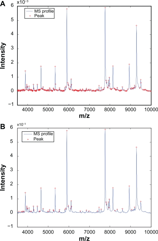
At this point we have not applied any additional constraints on the detected peaks. Therefore it is not surprising that massive amount of peaks will be detected from a typical mass spectrum. Indeed, for a mass spectrum taken from the prostate cancer data set, which contains 17817 m/z-intensity pairs, 1396 peaks have been identified. Figure 2(A) shows one segment of the mass spectrum along with the identified peaks, and we observe that the vast majority of the identified peaks have small magnitude and are close to baseline, which are the peaks prone to misalignment.
Figure 2.
Automatic detection of calibration peaks: A) Peaks detected without additional constraints; B) Peaks detected with additional constraints.
As pointed out in Section 2, the proposed alignment algorithm only align the peaks corresponding to high-abundance proteins in order to estimate the warping function accurately. To remove the small peaks, constraints on peak height is imposed to the detection procedure. In this work, we use the peaks whose magnitude are among the top 20% as the calibration peaks. For the prostate cancer example, after imposing the constraint, 1117 out of 1396 peaks are eliminated with only 279 peaks left. Figure 2(B) shows the detected peaks with the constraint. It can be seen that the detected peaks show clear distance from the baseline, which helps reducing misalignment. It is worth noting that even with the additional constraints in the detection procedure, it is likely that not all peaks detected in the reference spectrum will present in the test spectrum, which introduces potential difficulty for peak alignment. This difficulty can be addressed by SCW as discussed in the next two subsections.
Calibration peak alignment
For each calibration peak in the reference spectrum, we first determine the alignment window for the peak, then we shift the corresponding segment of the test spectrum to the left and the right in order to maximize the correlation coefficient between the two peak segments, and the shift that maximizes the correlation coefficient is set as the value of the warping function at the calibration point. The details of these steps are given below.
First we use an example to illustrate how to determine the alignment window for the reference spectrum. Figure 3(A) plots the segments of the reference and test spectra around a reference calibration peak. The solid line denotes the reference spectrum and the dashed line denotes the test spectrum. The calibration peak is highlighted with a thicker line. One natural choice of the alignment window width is simply the peak width, which is defined as the distance between the two valleys adjacent to the peak as shown in Figure 3(A). However, this choice could result in possible misalignment as shown in Figure 3(B), where two peaks with obvious different characteristics are seemingly aligned perfectly within the alignment window. To avoid such pitfall, we extend the alignment window on both sides to capture parts of the valleys adjacent to the calibration peak. In this work, we include 10 extra points on each side of the calibration peak. The alignment result in b) is replotted in c) with the extended alignment window, and it is easy to tell that the peaks in the reference and test spectra are misaligned. The correct alignment result is shown in Figure 3(D) with the extended alignment window, where A′ of the test spectrum is correctly aligned with A of the reference spectrum. Next we align the peak segment in the test spectrum with the reference spectrum within the alignment window. We shift the test spectrum in both directions within the allowed range (ie, the search window) in order to match the reference segment as closely as possible. In existing algorithms, both distance measures and correlation measures have been used to evaluate how well two segments are aligned.8 In this work, we choose the correlation measure as the alignment criterion. The correlation measure relies on the overall shape of the peak instead of the peak height to evaluate the alignment performance. Therefore it is a more robust indicator for peak alignment compared to the distance measure.
Figure 3.
Illustration of different alignment windows: A) Reference and test spectra before alignment; B) Alignment result with peak width as the window width; C) Misalignment revealed by expanded window; D) Correct alignment with the expanded window.
We use ni to denote the width of the alignment window for the ith calibration peak (in the number of measurement points, which is the peak width plus 20 in this work), and use xi to denote the m/z values that are included in the alignment window, ie,
| (1) |
In addition, we use r(xi) and t(xi) to denote the intensities of the peak segments in the reference and test alignment windows. Mathematically, the alignment process is to search for the optimal shift that maximize the correlation coefficient between the reference segment and the shifted test segment within the alignment window, ie,
| (2) |
with |Δi| ≤ θ, where ρ denotes the correlation coefficient between the reference and the test segments and θ denotes the search window width. It is clear that a positive Δi indicates shifting the test spectrum to the left and a negative Δi to the right. In addition, the value of the warping function w(·) at the apex of the ith calibration peak (ie, the ith calibration point) is set to .
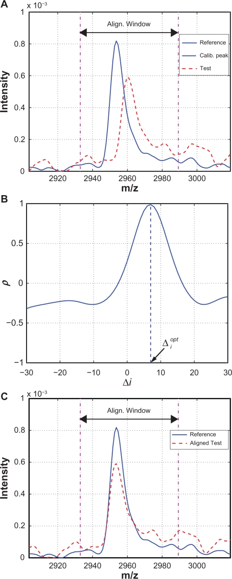
Figure 4 is an example used to illustrate the alignment procedure. Figure 4(A) shows the reference and test spectra around a calibration peak. Correlation coefficients between the reference segment and the shifted test segments are plotted in Figure 4(B) where x-axis is the shifting distance Δi. The maximum ρ is obtained with . Therefore, the test spectrum should be shifted to the left by 7 measurement points (or 6.92 in m/z unit) in order to be aligned with the reference peak. The aligned test and reference calibration peak are shown in Figure 4(C).
Figure 4.
Illustrative example: A) A test spectrum to be aligned with a calibration peak of the reference spectrum; B) ρ vs. Δi; C) After alignment based on .
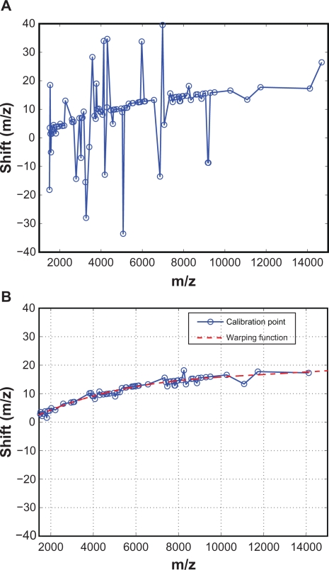
For a test spectrum, we perform the above alignment procedure for all calibration peaks identified in the reference spectrum, and obtain values of the warping function at the calibration points. Figure 5(A) shows an example of the obtained values of the warping function. It can be seen that the warping function has a dominant low-frequency component, but also has some big spikes. These spikes are likely caused by misalignment, as we expect that the warping function consists of low-frequency component only. In the next subsection, we investigate the causes of the spikes in the warping function, which turned out to be misalignments as expected, and we propose a predictor-corrector scheme to reduce such misalignments. The estimated warping function after applying the predictor-corrector scheme is shown in Figure 5(B), where all major spikes have been eliminated.
Figure 5.
Estimated warping function values at calibration points: A) Spikes in the warping function values due to misalignment; B) The predictor-corrector scheme eliminates potential misalignment.
Eliminating possible misalignment of calibration peaks
After examining the alignment of the calibration peaks corresponding to the spikes in Figure 5(A), we found that the spikes mainly occur in two cases and they are indeed caused by misalignment. One case is that there are multiple peaks in the test spectrum around the reference calibration peak; the other is that there is no obvious peak in the test spectrum around the reference calibration peak. Below we discuss how to eliminate possible misalignment in these two cases.
An example of misalignment in the first case is given in Figure 6, where (A) shows the reference and test spectra before alignment. Around the reference calibration peak, there are multiple peaks in the test spectrum, which results in multiple local maxima in the correlation coefficient curve within the search window ([−θ, θ ]). Figure 6(B) shows the correlation coefficient between the reference and the shifted test spectra within the search window ([−30, 30]), where the local maxima are labeled as A, B, C and D, with D being the global maximum. According to the alignment algorithm in Section 2.2.2, shift corresponding to D will be selected and the test spectrum will be shifted to the left by 29 points with the resulted alignment shown in Figure 6(C). Despite the good alignment of the reference and test segments within the alignment window, if we consider the spectrum segments outside of the alignment window it is clear that the test spectrum is misaligned. The correct alignment is shown in Figure 6(D), which actually corresponds to point B, a local maximum in Figure 6(B). Reducing the searching window width(ie, θ) can eliminate the misalignment in this case, but it comes with the risk of missing the optimal alignment for other calibration peaks. To address this difficulty, we propose a predictor-corrector scheme to automatically determine a much narrower, floating searching window, which effectively eliminates the possible misalignment without the risk of missing correct alignment. The predictor-corrector scheme is again based on the assumption that the warping f unction is a smooth function containing low-frequency components. Therefore, for the ith calibration peak, based on the optimal shifts associated with the calibration peaks that have been aligned, (ie, , , …, ), we use an exponentially weighted moving average (EWMA) filter, which is a low-pass filter, to predict the approximate location of the optimal shift , and reduce the searching window to a small neighborhood of , ie, [ , ] with θ′ << θ. Specifically, is obtained as follows,
| (3) |
where ω is the EWMA weighting. In this work, we set ω = 0.3 and θ′ = 3. For the example shown in Figure 6, the predicted optimal , which is shown as the circle close to the point B, and the floating searching window is reduced to,4,10 which is significantly narrower than the original searching window of [−30, 30]. Within the floating searching window, the optimal shift is correctly identified which corresponds to the local maximum B. In the case that no maximum exists within the floating searching window, the calibration peak will be removed from the list for the test spectrum, and will be not used to estimate the warping function.
Figure 6.
A) Segments to be aligned; B) Correlation coefficient ρ vs. shift Δi; C) Alignment based on the global maxima which is a misalignment; D) Correct alignment based on a local maxima.
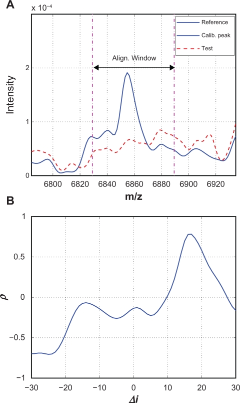
An example of the misalignment in the second case is shown in Figure 7 where there is no obvious peak in the test spectrum around a reference calibration peak. Figure 7(A) shows the reference and test spectra before alignment, and we observe that the test spectrum is dominated by random baseline fluctuations without obvious peaks. In this case, there is no good match between the reference and the shifted test segments, even at the optimal shift corresponding to the maximum correlation coefficient. Figure 7(B) shows the correlation coefficient curve for this example, where the maximum correlation coefficient ρmax = 0.78. In this case, the identified optimal shift is mainly caused by chance and should not be used to estimate the warping function. It is relatively easy to eliminate misalignment caused by missing peaks in the test spectrum. We add a lower bound to the maximum correlation coefficient, denoted by ρ̱. If ρmax < ρ̱, the calibration peak will be removed and will not be used to estimate the warping function. In this work, we set ρ̱ = 08. It is worth noting that this misalignment might have been prevented by the predictor-corrector if 17 does not fall within [ , ].
Figure 7.
A) One example where there is no corresponding calibration peak in the test spectrum; B) The “optimal” shift of 17 is caused by chance.
After implementing the predictor-corrector scheme and adding the lower bound on ρmax, the estimated values of the warping function at all calibration points are shown as circles in Figure 5(B). It can be seen that the misalignments are effectively removed, and the estimated warping function has a low-frequency trend.
Spectrum alignment
To align the whole spectrum, we first obtain the warping function w(x) over the whole m/z range of the spectrum, then shift the whole test spectrum t(x) according to the warping function, and the resulted spectrum, ie, t(x + w(x)), is expected to be better aligned to the reference spectrum r(x). To obtain w(x), we use a third-order polynomial to model the warping function, and the model parameters are estimated using the values of the warping function at the calibration points. Note that other (piecewise) functions can be used to model the warping function as well. In this work, w(x) is expressed as
| (4) |
To estimate the model parameters a0 ∼ a3, we apply a weighted least squares where each calibration point can be weighted differently according to peak magnitude or area, or other a priori information. In this work, we use the square root of the peak height as the weight for each calibration point. Figure 5(B) shows the fitted warping function (dashed line) based on the values obtained from the calibration points (circles), which shows that a third-order polynomial is adequate to describe the warping function.
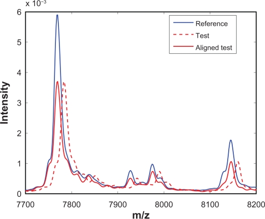
With the warping function w(x) available, it is straightforward to obtain the aligned spectrum, which is simply t(x + w(x)). Note that SCW does not insert or delete any measurement points from the raw spectrum, instead SCW simply shifts a measurement point to the left or to the right according to the warping function. Following alignment, the intensity of the aligned test spectrum at any given m/z value can be obtained easily through cubic spline interpolation or other interpolation methods. Figure 8 shows one segment of the test spectrum before alignment (red dashed line) and after alignment (red solid line). It can be seen that SCW is effective in synchronizing the test spectrum with the reference spectrum.
Figure 8.
A segment of test spectrum before and after alignment.
As the calibration peaks may not spread over the whole range of the mass spectrum, extra caution should be taken when calculating the warping function through extrapolation. In this work, for the segments at the both ends of a spectrum that do not contain any calibration peaks, we use a first-order polynomial to model the warping function. The slope of the linear function is determined by the slope of the fitted third-order polynomial at the boundary calibration points. For the example shown in Figure 5(B) where the m/z values are greater than 14000, a straight line is used to approximate the warping function. Without any calibration peaks located in the segment, the alignment accuracy is not guaranteed. However, by observing the whole spectrum, it appears that little protein/peptide is detected beyond m/z value of 14000. Therefore, even if misalignment occurred in this segment, it will have little effect on the subsequent analysis. In addition, it is worth noting that all existing alignment methods face the same problem and extreme stretching and compression have been observed in other methods for the segment where no significant peaks exist.
Results and Discussion
In this section, we first demonstrate the alignment performance of the SCW method using the prostate cancer data set; then we discuss some desirable properties of SCW; finally we compare SCW’s alignment performance with five representative alignment methods and we show that SCW reduces spectrum stretching and compression without sacrificing alignment performance. The methods we compared are: COW, DDTW, PTW, RAFFT, and MSA. For all five representative methods, we select the set of tuning parameters that optimize their alignment performance. Among these methods, only SCW and MSA require peak detection prior to alignment, while the rest four methods align spectrum segment directly.
Alignment performance of SCW
The clinical prostate cancer data set used in this study consists of SELDI-TOF mass spectra of blood serum from 317 normal control samples. The data set was generated from a validation study designed and performed by the Early Detection Research Network (EDRN).1–3 Each spectrum contains 17817 intensity-m/z pairs. The spectrum that has the highest average correlation with the rest of the spectra is selected as the reference spectrum.
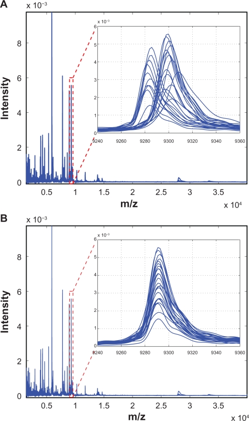
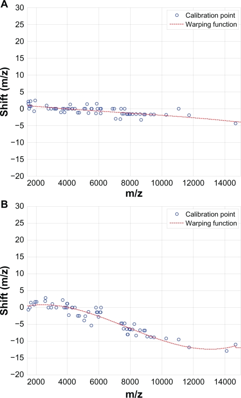
Figure 9 demonstrates the effectiveness of the proposed SCW alignment, where (A) shows 20 spectra before alignment and (B) after alignment. The insets are the zoom-in views of one peak before and after alignment. It can be seen that before alignment peaks are not synchronized, and after alignment the peaks are shifted appropriately to match the reference. Figure 10 shows two examples of warping function for different test spectra. It can be seen that the third-order polynomials adequately model the shifts in different spectra, and the proposed SCW method effectively eliminates possible misalignment because there is no major spikes show up in the warping function at the calibration points.
Figure 9.
20 SeLdI-ToF MS spectra before A) and after B) alignment using the proposed SCW method. The insets show the zoomed view of the indicated regions.
Figure 10.
Third-order polynomials adequately model the shifts in different spectra (A) and (B).
Desirable properties of SCW
There are several advantages associated with the SCW method. One advantage is its robustness. Because of the predictor-corrector mechanism used to determine the values of the warping function at the calibration points and the low-order polynomial fitting used to determine the overall warping functions, SCW is very robust and its performance is not sensitive to the tuning parameters. This property is highly desirable because it allows us to automate the alignment algorithm by using a fixed set of parameters, instead of requiring the user to tune the algorithm in order to obtain optimal performance. In this subsection we illustrate this property using the clinical prostate cancer dataset, and we show that a wide range of tuning parameters result in similar alignment performance.
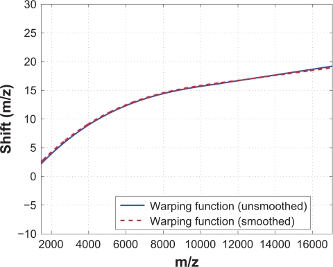
In the SCW method, there are three tuning parameters: 1) the percentage of peaks to be used as calibration peaks ( p); 2) the EWMA weighting (ω); and 3) the predictor-corrector search window (θ′). Figure 11 compares the warping functions obtained for a test spectrum with different parameter settings. In each subplot, we vary one parameter within a certain range while keeping the other two constant. We first vary the percentage of peaks used as calibration peaks, while keeping ω = 0.4 and θ′ = 4. The warping function obtained with different p’s are plotted in Figure 11(A), which shows that the alignment performance does not change noticeably for a wide range of p (between 15% and 40%). Similar comparison are performed to examine the effect ω of and θ′. Figure 11(B) and (C) show that a wide range of ω and θ′ give almost identical alignment performance. Another advantage of SCW is that it is not sensitive to the noise level in the spectrum. We demonstrate this by showing that the alignment performance does not change much if the reference and test spectra are not smoothed before alignment. Figure 12 compares the estimated warping functions of a test spectrum based on different preprocessing procedures: one with smoothing and the other without. In both cases, baseline correction is performed for the reference and test spectra. In Figure 12 the solid line represents the warping function obtained based on the unsmoothed data and the dashed line is based on the smoothed data. We can see that the two warping functions are almost identical. In addition, we compare the correlation coefficients of the test spectrum and the reference spectrum before and after alignment for both cases, and the result is shown in Table 1. Both Figure 12 and Table 1 show that without spectrum smoothing, the performance of the SCW method is almost not affected. The most significant advantage of SCW is that it reduces spectrum stretching/compression without sacrificing alignment performance, which is discussed in more detail in the next subsection where SCW is compared with five other methods. Other advantages of SCW include its fast computation speed, low memory requirement and flexibility. In addition, the SCW method does not require the reference and the test spectra to have the same sequence of m/z values. Therefore, the SCW method can be directly applied to align spectra obtained from different batches or different laboratories.
Figure 11.
The performance of the SCW method is robust with respect to different tuning parameters. A) effect of p; B) effect of ω; C) effect of θ′.
Figure 12.
Warping functions based on smoothed (solid line) and unsmoothed (dashed line) data are similar, which indicates that SCW is not sensitive to the noise level in the spectra.
Table 1.
Correlation coefficients between the test and the reference spectrum.
| Before alignment | After alignment | |
|---|---|---|
| Smoothed | 0.6245 | 0.9401 |
| Unsmoothed | 0.6194 | 0.9383 |
Comparison of SCW with other methods
In this subsection we compare the performance of SCW with five other alignment methods using the clinical prostate cancer data set introduced in Section 3.1. The alignment performance is first quantified by comparing the alignment precision, correlation coefficients between the reference and aligned test spectra, and the computation time of different methods; then the quality of the alignment is evaluated visually using an example to illustrate possible peak misalignment and peak shape deformation.
Quantitative comparison
The alignment performance from different algorithms are first assessed quantitatively by the average alignment precision for the top 50 peaks according to the peak height. The alignment precision for the ith peak is defined as:
| (5) |
where di denotes the distances between the apices of the ith peak in the reference and the 316 aligned test spectra (in the unit of sample points). The average alignment precision of the top 50 peaks for different methods are listed in Table 2. In addition, the average correlation coefficients between the reference and the 316 aligned test spectra for different methods are listed in Table 3. Both Tables 2 and 3 show that all alignment methods are effective in aligning test spectra. In addition, in terms of the alignment precision and correlation coefficient improvement, SCW performs slightly worse than DDTW, and slightly better than COW, MSA, PTW and RAFFT.
Table 2.
Comparison of alignment precision of the 50 most intense peaks.
| None | SCW | COW | DDTW | PTW | RAFFT | MSA |
|---|---|---|---|---|---|---|
| 5.09 ± 3.11 | 1.25 ± 1.17 | 1.52 ± 1.51 | 1.04 ± 1.14 | 1.36 ± 1.23 | 1.32 ± 1.19 | 1.42 ± 1.26 |
Table 3.
Comparison of correlation coefficients between the reference and aligned test spectra.
| None | SCW | COW | DDTW | PTW | RAFFT | MSA |
|---|---|---|---|---|---|---|
| 0.902 | 0.932 | 0.926 | 0.934 | 0.927 | 0.930 | 0.923 |
Finally the computation time required by different methods are compared based on aligning a single spectrum of 17817 intensity-m/z pairs. All computations are carried out on a laptop equipped with Intel dual core 1.20 GHz processor and 1.5 GB of RAM. The results are listed in Table 4, which shows that COW and DDTW take significantly longer time because they make use of dynamic programming. All other 4 methods use few seconds or even shorter time to align a spectrum with about 18k measurements. Note that due to insufficient memory, the computation time of DDTW is estimated by scaling the computation time required for aligning 1/4 of the whole spectrum with the factor of 16.12 Fast computation is desirable because it allows the alignment methods to be applied to large MS data set which are becoming increasingly common.
Table 4.
Comparison of computation time for aligning a single spectrum with 17817 measurements.
| Algorithm | SCW | COW | DDTW | PTW | RAFFT | MSA |
|---|---|---|---|---|---|---|
| Time (sec) | 2.4 | 237.4 | 1307.2 | 0.1 | 0.6 | 5.9 |
Qualitative comparison
In this subsection we show that SCW introduces the least distortion to the raw spectra among all the six alignment methods. This is critical for the subsequent analysis steps such as biomarker identification, because biological information contained in the spectra is better conserved with less manipulation. To examine the details of different alignment methods, we use one test spectrum to illustrate the warping functions obtained from different methods and compare their alignment result qualitatively.
-
Correlation optimized warping (COW)
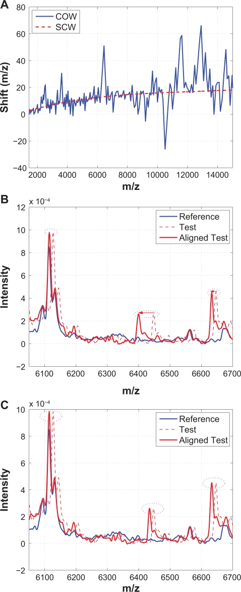
COW aligns spectra by means of piecewise linear stretching and compression to maximize the summed correlation coefficients of all segments. Details of COW can be found in,8 and the Matlab code was downloaded from http://www.models.kvl.dk.10 Figure 13 compares the performance of COW and SCW using an example. Specifically, Figure 13(A) plots segments of warping functions obtained from COW (solid line) and SCW (dashed line), Figure 13(B) plots a segment of the reference spectrum, the test spectrum before and after alignment from COW, and Figure 13(C) plots the same segments from SCW. Figure 13 indicates that COW introduces many over-stretching and over-compression as indicated by the frequent spikes in the obtained warping function, which is also illustrated in Figure 13(B) where the shifts among three neighboring peaks are significantly different from each other. Nevertheless, the warping functions obtained from COW and SCW seem to follow the same low frequency trend as shown in Figure 13(A).
-
Derivative dynamic time warping (DDTW)
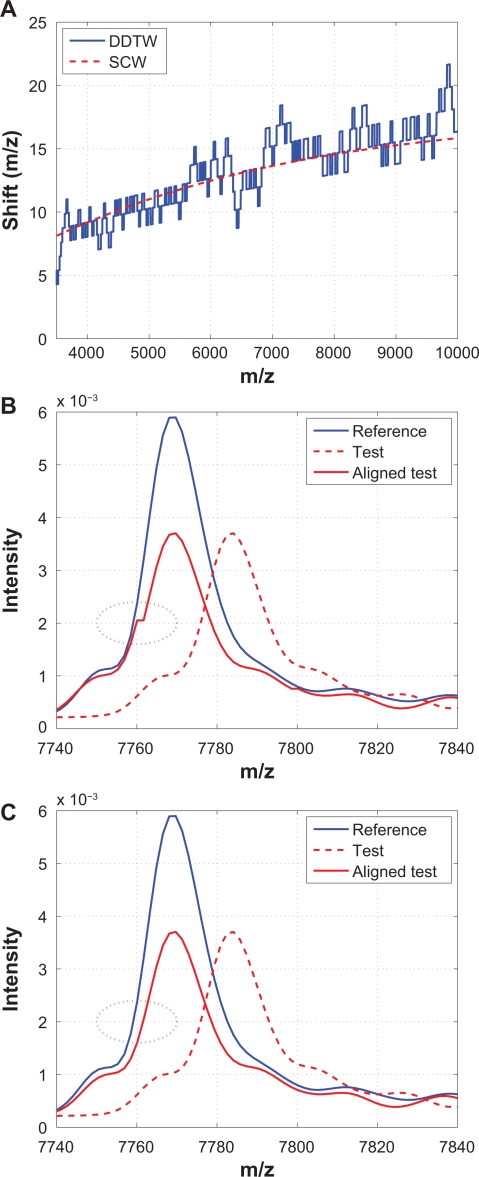
It has been shown that DDTW produces superior alignment than the classic dynamic time warping (DTW) algorithm.22 Therefore, only DDTW is considered in this study. The local derivative estimation is based on,22 and the classic DTW algorithm (Matlab code downloaded from http://www.models.kvl.dk)10 is applied to align the derivatives. The warping function obtained based on the derivatives is then used to align the original spectra. Figure 14 compares DDTW and SCW using the same example that was shown in Figure 13. From Figure 14(A) we observe that warping functions obtained from both algorithms follow the same low frequency trend, but the one from DDTW has frequent switches between stretching and compressing. Because of these excessive stretching and compression, artifacts such as a small “stair” could be introduced to the shifted spectrum, as shown in (B), which SCW does not suffer from. The “stair” in Figure 14(B) is also called “singularity” where a single point on one spectrum is mapped onto multiple points of another spectrum, and singularities are also present in other methods that make use of dynamic programming, such as DTW and COW. It should be noted that singularities are not desirable because peak widths and peak areas are altered from the original spectrum, which may change the biological information contained in the original spectrum.
-
Parametric time warping (PTW)
PTW aligns spectra by means of modeling the warping function as a polynomial to minimize the distance between two spectra.9 The Matlab code of PTW is downloaded from http://www.bdagroup.nl/.25 Among the methods we compared in this work, PTW and SCW are similar in the sense that PTW uses a second-order polynomial while SCW uses a third-order polynomial to model the warping function. However, besides the order of the polynomial used to model the warping function, there are other differences between them. The most important one is that SCW only aligns calibration peaks while PTW aligns the whole spectrum to estimate the polynomial parameters, which is prone to baseline noise. In addition, SCW uses a correlation measure while PTW uses a distance measure as the alignment criterion, therefore PTW may suffer from the same problems as other distance-based algorithms such as DTW. For example, misalignment could occur simply because a peak in one spectrum is more or less intense than its corresponding feature in the other spectrum.22 Finally, SCW has guaranteed convergence because it separates calibration peak alignment from warping function parameter estimate, while in PTW, due to integrated spectrum alignment and parameter estimation, sharp peaks have to be artificially broadened by strong smoothing in order to get successful convergence.9
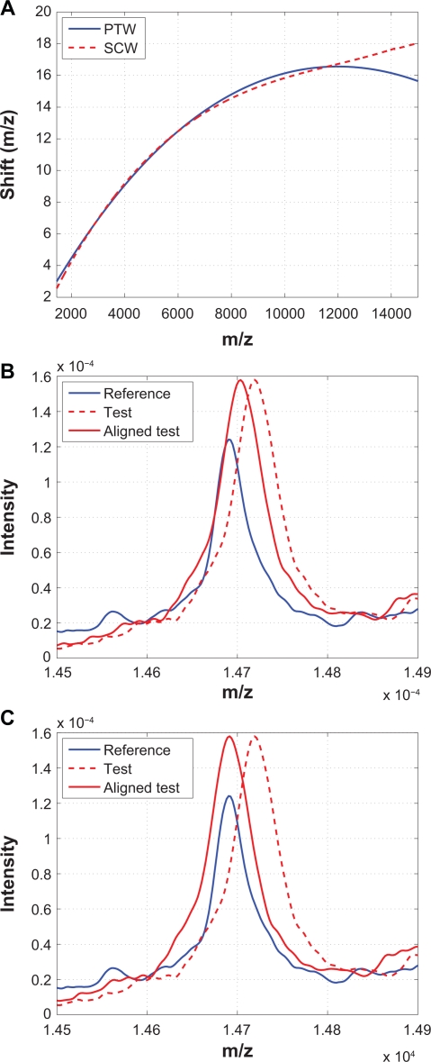
Figure 15 compares PTW and SCW. The alignment results obtained from these two methods are remarkably similar to each other for m/z values less than 12000. However, for larger m/z values, PTW seems to have some difficulty in obtaining optimal alignment, as shown in (B) and (C), which may be due to the limitation of the second order polynomial warping function.
-
Recursive alignment by fast Fourier transform
There are two alignment algorithms developed based on fast Fourier transform. One makes use of the beam search segmentation model, and the other implements a recursive segmentation model. The Matlab codes of both algorithms can be downloaded from http://physchem.ox.ac.uk/~jwong.12,13
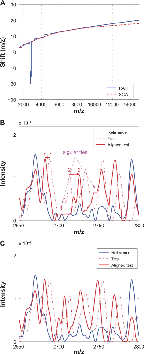
Because it has been shown that the recursive algorithm (RAFFT) performs better in,12 only the RAFFT results are provided. Figure 16 compares RAFFT with SCW. Again, Figure 16(A) shows that the warping functions obtained from RAFFT and SCW are remarkable similar to each other, except for one small segment that is shown in (B) and (C), where obvious singularities are introduced by RAFFT.
-
MSAlign from Matlab Bioinformatics Toolbox (MSA)
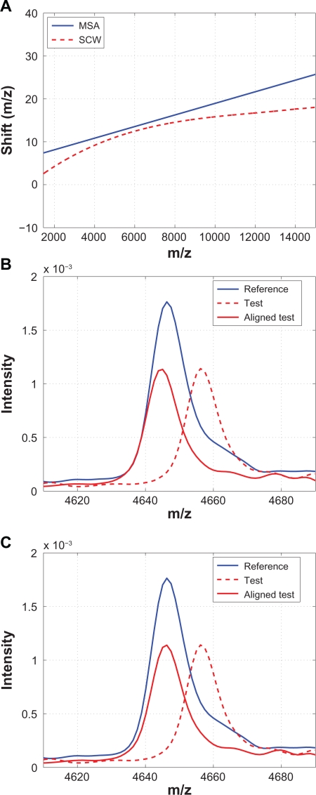
MSA aligns a spectrum based on peak alignment, and it requires the user to identify the signature peak locations as the input to the alignment algorithm. It linearly scales and shifts the domain (ie, m/z values) such that the cross-correlation between the test spectrum and a synthetic reference spectrum is maximized.23 Among the methods compared, MSA and SCW are the only methods that implement peak alignment. However, MSA requires the user to manually identify the peaks to be aligned, and it models the warping function as a first-order polynomial, ie, a straight line, which may result in limitations when applied to clinical data sets. Figure 17 compares the results from MSA with SCW. Because of the simple model that MSA adopts for the warping function, it is expected to see some peaks that are not properly aligned as the one shown in Figure 17(B).
Figure 13.
Comparison of COW with SCW: A) Warping functions obtained from COW and SCW; B) A segment showing that shifts among three neighboring peaks are significantly different in COW; C) The same segment aligned by SCW where shifts among three neighboring peaks are similar.
Figure 14.
Comparison of DDTW with SCW: A) Warping functions obtained from DDTW and SCW; B) A segment showing that a “stair” is introduced during alignment thus the peak widths and areas are altered by DDTW; C) The same segment aligned by SCW where no “stair” is introduced.
Figure 15.
Comparison of PTW with SCW: A) Warping functions obtained from PTW and SCW; B) A segment showing that some peaks are not aligned properly by PTW; C) The same segment aligned by SCW.
Figure 16.
Comparison of RAFFT with SCW: A) Warping functions obtained from RAFFT and SCW; B) A segment showing that two neighboring peaks (1 and 2) are shifted to opposite directions during the alignment which results in obvious singularity; C) The same segment aligned by SCW.
Figure 17.
Comparison of MSA with SCW: A) Warping functions obtained from MSA and SCW; B) A segment showing that some peaks are not aligned properly by MSA if they are not included as the candidate peaks; C) The same segment aligned by SCW.
Conclusion
In this work we present a new spectrum alignment method, ie, self-calibrated warping, and compare it with five other alignment methods using a clinic prostate cancer data set. The SCW method has many advantages. Instead of aligning the whole spectrum, it aligns calibration peaks only to identify the value of a warping function at calibration points, then estimate the warping function over the whole range using a third-order polynomial function. In this way, SCW avoids direct alignment of segments that contain small and dense peaks, therefore reducing possible misalignment significantly. In addition, SCW is very robust and not sensitive to the tuning parameters and the noise level in the spectra. This is because SCW implements a predictor-corrector scheme to align calibration peaks. The predictor-corrector scheme determines the search window on-the-fly, which significantly narrows the search window and eliminates possible misalignment. Moreover, SCW uses a third-order polynomial to model the warping function over the whole range of the spectrum. The smoothness of the polynomial function prevents possible over-stretching and over-compression, especially for segments consisting of small and dense peaks. Finally, SCW’s relatively fast computation and low memory consumption allowing its application to large data set that are becoming increasingly common. These features make SCW a user friendly and reliable tool for spectrum pre-processing. It is worth noting that although the algorithm is developed based on a MS data set, it is generally applicable to other fields where signal alignment is required or desired, such as chromatography, nuclear magnetic resonance (NMR) spectroscopy, Raman spectroscopy and NIR spectroscopy. The Matlab code of SCW will be provided for research purposes upon request.
Acknowledgments
The financial support from NSF under the grants CBET 0853748 (QPH) and CBET-0853983 (JW) is greatly appreciated.
Footnotes
Disclosures
This manuscript has been read and approved by all authors. This paper is unique and not under consideration by any other publication and has not been published elsewhere. The authors and peer reviewers report no conflicts of interest. The authors confirm that they have permission to reproduce any copyrighted material.
References
- 1.Semmes OJ, Feng Z, Adam B-L, et al. Evaluation of serum protein profiling by surface-enhanced laser desorption/ionization time-of-flight mass spectrometry for the detection of prostate cancer: I. assessment of platform reproducibility. Clin Chem. 2005;51:102–12. doi: 10.1373/clinchem.2004.038950. [DOI] [PubMed] [Google Scholar]
- 2.McLerran D, Grizzle WE, Feng Z, et al. Analytical validation of serum proteomic profiling for diagnosis of prostate cancer: Sources of sample bias. Clin Chem. 2008;54:44–52. doi: 10.1373/clinchem.2007.091470. [DOI] [PMC free article] [PubMed] [Google Scholar]
- 3.McLerran D, Grizzle WE, Feng Z, et al. SELDI-TOF MS whole serum proteomic profiling with IMAC surface does not reliably detect prostate cancer. Clin Chem. 2008;54:53–60. doi: 10.1373/clinchem.2007.091496. [DOI] [PMC free article] [PubMed] [Google Scholar]
- 4.Sauve A, Speed T. Normalization, baseline correction and alignment of high-throughput mass spectrometry data. Proceedings of the Genomic Signal Processing and Statistics; Baltimore, MD. [Google Scholar]
- 5.Jeffries N. Algorithms for alignment of mass spectrometry proteomic data. Bioinformatics. 2005;21:3066–73. doi: 10.1093/bioinformatics/bti482. [DOI] [PubMed] [Google Scholar]
- 6.Malyarenko DI, Cooke WE, Adam B-L, et al. Enhancement of sensitivity and resolution of surface-enhanced laser desorption/ionization time-of-flight mass spectrometric records for serum peptides using time-series analysis techniques. Clin Chem. 2005;51:65–74. doi: 10.1373/clinchem.2004.037283. [DOI] [PMC free article] [PubMed] [Google Scholar]
- 7.Baggerly KA, Morris JS, Coombes KR. Reproducibility of SELDITOF protein patterns in serum: comparing datasets from different experiments. Bioinformatics. 2004;20:777–85. doi: 10.1093/bioinformatics/btg484. [DOI] [PubMed] [Google Scholar]
- 8.Nielsen NPV, Carstensen JM, Smedsgaard J. Aligning of single and multiple wavelength chromatographic profiles for chemometric data analysis using correlation optimized warping. Journal of Chromatography A. 1998;805:17–35. [Google Scholar]
- 9.Eilers PHC. Parametric time warping. Analytical Chemistry. 2004;76:404–11. doi: 10.1021/ac034800e. [DOI] [PubMed] [Google Scholar]
- 10.Tomasi G, van den Berg F, Andersson C. Correlation optimized warping and dynamic timewarping as preprocessing methods for chromatographic data. Journal of Chemometrics. 2004;18:231–41. [Google Scholar]
- 11.Van Nederkassel A, Daszykowski M, Eilers P, Heyden YV. A comparison of three algorithms for chromatograms alignment. Journal of Chromatography A. 2006;1118:199–210. doi: 10.1016/j.chroma.2006.03.114. [DOI] [PubMed] [Google Scholar]
- 12.Wong JWH, Durante C, Cartwright HM. Application of fast fourier transform cross-correlation for the alignment of large chromatographic and spectral datasets. Analytical Chemistry. 2005;77:5655–61. doi: 10.1021/ac050619p. [DOI] [PubMed] [Google Scholar]
- 13.Wong JW, Cagney G, Cartwright HM. Specalign–processing and alignment of mass spectra datasets. Bioinformatics. 2005;21:2088–90. doi: 10.1093/bioinformatics/bti300. [DOI] [PubMed] [Google Scholar]
- 14.Torgrip RJO, Aberg M, Karlberg B, Jacobsson SP. Peak alignment using reduced set mapping. Journal of Chemometrics. 2003;17:573–82. [Google Scholar]
- 15.Forshed J, Schuppe-Koistinen I, Jacobsson SP. Peak alignment of nmr signals by means of a genetic algorithm. Anal Chim Acta. 2003;487:189–99. [Google Scholar]
- 16.Lee GC, Woodruff DL. Beam search for peak alignment of NMR signals. Anal Chim Acta. 2004;513:413–6. [Google Scholar]
- 17.Forshed J, Torgrip RJ, Åberg KM, Karlberg B, Lindberg J, Jacobsson SP. A comparison of methods for alignment of nmr peaks in the context of cluster analysis. Journal of Pharmaceutical and Biomedical Analysis. 2005;38:824–32. doi: 10.1016/j.jpba.2005.01.042. [DOI] [PubMed] [Google Scholar]
- 18.Booksh KS, Stellman CM, Bell WC, Myrick ML. Mathematical alignment of wavelength-shifted optical spectra for qualitative and quantitative analysis. Appl Spectrosc. 1996;50:139–47. [Google Scholar]
- 19.Witjes H, van den Brink M, Melssen WJ, Buydens LMC. Automatic correction of peak shifts in raman spectra before pls regression. Chemometrics and Intelligent Laboratory Systems. 2000;52:105–16. [Google Scholar]
- 20.Witjes H, Pepers M, Melssen WJ, Buydens LMC. Modelling phase shifts, peak shifts and peak widthvariationsin spectral data sets: its value in multivariate data analysis. Analytica Chimica Acta. 2001;432:113–24. [Google Scholar]
- 21.Pravdova V, Walczak B, Massart DL. A comparison of two algorithms for warping of analytical signals. Analytica Chimica Acta. 2002;456:77–92. [Google Scholar]
- 22.Keogh EJ, Pazzani MJ. Derivative dynamic time warping. First SIAM International Conference on Data Mining; Chicago, IL. [Google Scholar]
- 23.Matlab bioinformatics toolbox. 2008. www.mathworks.com.
- 24.Zhang Y, Edgar TF. A robust dynamic time warping algorithm for batch trajectory synchronization. Proc. American Control Conference; Seattle, WA. 2008. pp. 2864–9. [Google Scholar]
- 25.Ramaker HJ, van Sprang ENM, Westerhuis JA, Smilde AK. Dynamic time warping of spectroscopic batch data. Analytica Chimica Acta. 2003;498:133–53. [Google Scholar]


