Genome-Wide Meta-Analysis of Joint Tests for Genetic and Gene-Environment Interaction Effects

Abstract

Background

There is growing interest in the study of gene-environment interactions in the context of genome-wide association studies (GWASs). These studies will likely require meta-analytic approaches to have sufficient power.

Methods

We describe an approach for meta-analysis of a joint test for genetic main effects and gene-environment interaction effects. Using simulation studies based on a meta-analysis of five studies (total n = 10,161), we compare the power of this test to the meta-analysis of marginal test of genetic association and the meta-analysis of standard 1 d.f. interaction tests across a broad range of genetic main effects and gene-environment interaction effects.

Results

We show that the joint meta-analysis is valid and can be more powerful than classical meta-analytic approaches, with a potential gain of power over 50% compared to the marginal test. The standard interaction test had less than 1% power in almost all the situations we considered. We also show that regardless of the test used, sample sizes far exceeding those of a typical individual GWAS will be needed to reliably detect genes with subtle gene-environment interaction patterns.

Conclusion

The joint meta-analysis is an attractive approach to discover markers which may have been missed by initial GWASs focusing on marginal marker-trait associations.

Introduction

There is considerable enthusiasm for genome-wide gene-environment interaction studies, in part because such studies may uncover causal loci which marginal tests have low power to detect [1]. However, standard statistical tests for gene-environment interaction, based on departures from additivity on some scale, also require large sample sizes to have reasonable power. Some researchers have developed statistical methods to increase the power of these standard tests by leveraging additional assumptions, such as gene-environment independence in the sampled population [2, 3, 4]. We have proposed a joint test of both the genetic main effect and gene-environment interaction parameters that can be more powerful than either the marginal or standard interaction tests when the genetic effect is weak in one exposure stratum but strong in another [5].

Still, regardless of the test used, the sample sizes required to reliably detect what are likely to be subtle effects will be quite large – larger than typically available in any single study. Hence, detecting gene-environment interactions will likely require a meta-analytic approach, as has been necessary for the identification of smaller and smaller marginal genetic effects. Meta-analysis of a single gene-environment interaction parameter is straight-forward: just as with meta-analyses of marginal additive effects, one could use an inverse-variance weighted fixed-effect approach, for example [6, 7]. Meta-analysis of multiple parameters, required for the joint test, is less well known. Here we derive a general approach to simultaneously estimate global fixed effects for multiple parameters and test whether they are identically null. Specifically, we consider models with genetic main effect plus gene-environment interaction parameters, or, equivalently, models with separate genetic effect parameters for each exposure stratum. We also present a computationally simpler version of this approach in the special case where the exposure is categorical. Using simulation we show that this meta-analysis approach provides valid tests of the null hypothesis that a marker is not associated with a trait in any exposure stratum. We also explore the power of this test over a wide range of models consistent with genetic effects that have been observed in recent genome-wide association studies (GWASs).

Methods

Let ${\stackrel{‸}{\beta }}_i\hspace{0.17em}=\hspace{0.17em}{({\stackrel{‸}{\beta }}_{g.i},\hspace{0.17em}{\stackrel{‸}{\beta }}_{g\hspace{0.17em}e.i})}^{\prime }$ be the vector of estimated genetic main and gene-environment interaction effects from study i, obtained from fitting the generalized linear model:

$$g(E[Y])\hspace{0.17em}=\hspace{0.17em}\alpha \hspace{0.17em}+\hspace{0.17em}{\beta }_{g}G\hspace{0.17em}+\hspace{0.17em}{\beta }_{e}E\hspace{0.17em}+\hspace{0.17em}{\beta }_{ge}G\hspace{0.17em}\times \hspace{0.17em}E.$$ [A]

For example, for a continuous outcome, the link function g(x) = x is equivalent to standard linear regression, and for a binary outcome, the link g(x) = log(x/(1 – x)) is equivalent to logistic regression. For ease of exposition, the genotype is assumed to be coded additively (0, 1, or 2 copies of the minor allele) and the exposure is assumed to be binary, so that ${\stackrel{‸}{\beta }}_{g\hspace{0.17em}e.i}$ is a scalar. The results are easily extended to categorical exposure with three or more levels, for example.

We note that for continuous exposures, both standard and joint tests can be invalid when the exposure main effect is mis-specified [8, 9]. Using the Huber-White robust ‘sandwich’ estimate of the variance-covariance matrix of ${\stackrel{‸}{\beta }}_i$ yields valid tests even when the continuous exposure is not modeled accurately. These robust covariance matrices are currently available from some software packages (e.g. ProbABEL [10]), but not others (e.g. PLINK [11]). Alternatively, breaking the continuous variable into categories (e.g. a binary indicator for high versus low exposure) also yields valid tests [8].

Following the exposition in van Houwelingen et al. [12] and assuming the sample size in every study is large enough so that ${\stackrel{‸}{\beta }}_i$ is multivariate normal with variance-covariance matrix Σ_i, we can write the log likelihood for the observed ${\stackrel{‸}{\beta }}_i$ as:

$$l(\beta )=-\hspace{0.17em}\frac{1}{2}\Sigma {(\beta -{\stackrel{‸}{\beta }}_i)}^T{\Sigma }_i^{-1}(\beta -{\stackrel{‸}{\beta }}_i)+k.$$

One can solve for the maximum likelihood estimate $\stackrel{‸}{\beta }$ using the score estimating equation

$$U(\beta )=\Sigma {[}^{{\Sigma }_i^{-1}}(\beta \hspace{0.17em}-\hspace{0.17em}{\stackrel{‸}{\beta }}_i)]=0.$$

This leads to the weighted least square solution:

$$\stackrel{‸}{\beta }\hspace{0.17em}=\hspace{0.17em}{[{\Sigma }^{{\Sigma }_i^{-1}}]}^{-1}[{\Sigma }^{{\Sigma }_i^{-1}}{\stackrel{‸}{\beta }}_i]$$

Given $\stackrel{‸}{\beta }$, the Wald test of the joint null β = 0 is $\beta \hspace{0.17em}=\hspace{0.17em}0\hspace{0.17em}\text{is}\hspace{0.17em}{\stackrel{‸}{\beta }}^{\text{T}}\hspace{0.17em}\text{I}\hspace{0.17em}\stackrel{‸}{\beta }$, where $\text{I}\hspace{0.17em}=\hspace{0.17em}{\Sigma }^{{\Sigma }_i^{-1}}$ is the Fisher information.

The score test also has a simple form:

$${({\Sigma }^{{\Sigma }_i^{-1}}{\stackrel{‸}{\beta }}_i]}^T\hspace{0.17em}{\text{I}}^{-1}({\Sigma }^{{\Sigma }_i^{-1}}{\stackrel{‸}{\beta }}_i).$$ [B]

Both of these tests have a non-central χ² distribution with 2 d.f. under the null hypothesis. (The assumption of normality is used here to motivate the estimation procedure; the test remains valid if the estimates ${\stackrel{‸}{\beta }}_i$ and Σ_i are unbiased but not normally distributed. Due to the consistency and asymptotic normality of maximum likelihood estimates, the study-specific estimates are likely unbiased and normally distributed when the individual sample sizes are ‘large enough’. Care should be taken when some studies have relatively small sample sizes, e.g. under 100 subjects.)

Although in principle this procedure yields valid and efficient tests of the joint null, in practice it may be difficult to implement, as it requires the covariance of ${\stackrel{‸}{\beta }}_{g.i}$ and ${\stackrel{‸}{\beta }}_{g\hspace{0.17em}e.i}$. Standard packages for the analysis of GWAS data such as PLINK [11] or glu (http://code.google.com/p/glu-genetics/) do not report this covariance without custom modification. (The --robust option in ProbABEL [10] will produce estimates of the variance-covariance matrix.) To avoid this complication, one might conduct a stratified analysis in each study, i.e. estimate the genetic effect in the exposed subjects ${\stackrel{‸}{\beta }}_{g.i}^{exp}$ and the effect in unexposed ${\stackrel{‸}{\beta }}_{g.i}^{\text{unexp}}$ separately. Since these estimates are uncorrelated (they are constructed using non-overlapping sets of subjects), the score test simplifies to:

$$\frac{{(\Sigma w_{g.i}^{exp}{\stackrel{‸}{\beta }}_{g.i}^{exp})}^2}{\Sigma w_{g.i}^{exp}}\hspace{0.17em}+\hspace{0.17em}\frac{{(\Sigma w_{g.i}^{\text{unexp}}{\stackrel{‸}{\beta }}_{g.i}^{\text{unexp}})}^2}{\Sigma w_{g.i}^{\text{unexp}}},$$ [C]

where

$$w_{g.i}^{exp}\hspace{0.17em}=\hspace{0.17em}\text{v}\stackrel{‸}{\text{a}}\text{r}{({\stackrel{‸}{\beta }}_{g.i}^{exp})}^{-1}$$

and $w_{g.i}^{\text{unexp}}\hspace{0.17em}=\hspace{0.17em}\text{v}\stackrel{‸}{\text{a}}\text{r}{({\stackrel{‸}{\beta }}_{g.i}^{\text{unexp}})}^{-1}.$

Note that expression [C] is simply the sum of the usual fixed-effect (inverse-variance weighted) tests for ${\stackrel{‸}{\beta }}_g^{exp}\hspace{0.17em}=\hspace{0.17em}0\hspace{0.17em}\text{and}\hspace{0.17em}{\stackrel{‸}{\beta }}_g^{\text{unexp}}\hspace{0.17em}=\hspace{0.17em}0$.

To demonstrate this approach, we used genotype data from five GWASs conducted using European-ancestry subjects: case-control studies of breast cancer (BRCA), type 2 diabetes (T2D) and coronary heart disease (CHD) in the Nurses’ Health Study (NHS), and case-control studies of T2D and CHD in the Health Professionals Follow-up Study (HPFS) [13, 14]. For each subject in each GWAS, a continuous phenotype Y was simulated as a function of two single nuclear polymorphisms (SNP) and one binary environmental exposure:

$$Y\hspace{0.17em}=\hspace{0.17em}a\hspace{0.17em}+\hspace{0.17em}{b}_{\text{E}}\hspace{0.17em}E\hspace{0.17em}+\hspace{0.17em}{b}_{\text{G}1}\hspace{0.17em}G1\hspace{0.17em}+\hspace{0.17em}{b}_{\text{G}2}\hspace{0.17em}G2\hspace{0.17em}+\hspace{0.17em}{b}_{\text{G2E}}\hspace{0.17em}{G}_2\hspace{0.17em}\times \hspace{0.17em}E\hspace{0.17em}+\hspace{0.17em}\epsilon$$

where G1 was the (observed) count of minor alleles for rs505922 (frequency from 34.1 to 35.8% in these studies), G2 was the (observed) count of minor alleles for rs1219648 (frequency from 39.6 to 42.0% in these studies), the exposure E was a Bernoulli 0-1 variable with expectation 0.3, and the residual variation ∊ was normally distributed with mean 0 and standard deviation σ. E and ∊were independent of each other as well as G1 and G2; since rs505922 is on chromosome 9 and rs1219648 is on chromosome 10, G1 and G2 were also effectively independent. We chose this model to examine the performance of the joint meta-analysis (and the marginal and standard interaction meta-analyses) in two situations: one where the effect does not differ across the exposure strata, and one where it does. The two SNPs were chosen arbitrarily, but are representative of the markers present on genome-wide genotyping platforms (rs505922 is on the Affymetrix Axiom and Illumina HumanHap550 arrays, among others, and rs1219648 is on the Affymetrix 6.0, Illumina HumanHap550, and Illumina OmniExpress arrays, among others).

To illustrate the validity of the meta-analytic joint test, we conducted a GWAS of a single realization of Y. This GWAS included 2,543,290 genotyped or imputed SNPs distributed along the 22 autosomal chromosomes that were available for all of the five studies. Because most of these SNPs are not in linkage disequilibrium with G1 or G2 and hence are not associated with the simulated phenotype, results from tests of the phenotype can be used to estimate the type I error rate of the meta-analytic approaches. For this example, the parameters b = (b_E, b_G1, b_G2, b_G2E)’ and σ were chosen so that the marginal test of G1 would have high power at the 5 × 10⁻⁸ level in the total sample (n = 10,161), and the joint gene-environment test of G2 would have high power in the total sample, while the marginal test of G2 would have modest or low power. The values b = (0.05, 0.12, 0.05, 0.10)andσ = 1.00 satisfied these criteria. Under this model, the genetic variants explained 0.9% of the variation in Y (0.7% for G1 and 0.2% for G2). We estimated subsequently the power of the meta-analytic joint test (and the marginal and standard interaction meta-analyses test) to detect G1 and G2 in this specific situation, by generating 100,000 realizations of Y with these parameters.

To further exemplify the power of the meta-analytic joint test relative to meta-analytic marginal and standard 1 d.f. interaction tests across a broad range of situations, we simulated 1,000 realizations of Y under each of 320 different parameter settings. We kept the values of b_G1, and σ fixed at their values in the previous simulation (0.12 and 1.00, respectively), while we varied b_E, b_G2 and b_G2E across a grid defined by b_E ∈ {0.05, 0.1, 0.5, 1, 2}, b_G2 ∈ {0.01, 0.04, 0.07, 0.1}, and b_G2E ∈ {−0.15 to 0.15 by 0.2 step}.

As these studies were conducted using different genotyping platforms (the Illumina 550k for the breast cancer study and Affymetrix 6.0 for the other four studies), we imputed missing genotypes using MACH [15] and the HapMap (rel22) CEU data. We conducted GWAS for SNPs associated with Y using ProbABEL, which takes the dosage files from MACH as input. We compared three tests. In the first test, we estimated the marginal effect of each SNP in each study, and then combined these estimates using standard fixed-effect meta-analysis. In the second, we estimated the usual product interaction term in each study (adjusting for SNP and exposure main effects), and then combined the estimates of these parameters using fixed-effect meta-analysis. In the final test, we estimated SNP effects stratified by study and exposure, and calculated the overall joint test using expression [C] above. We also investigated the effect of conditioning on a main effect for E (but not including a G × E interaction term) on the performance of the marginal tests for G1 and G2.

Results

Estimated type I error derived from the genome-wide association of more than 2.5 million SNPs with a single realization of Y are presented in table 1. This table shows the observed and the expected count of false positive tests for seven different p value thresholds. The observed counts are very close to those expected under the null hypothesis of no association. For example, for a p value threshold of 0.001, we expect a total of 2,537 false positives for the joint test and we observed 2,550, which is equivalent to an empirical p value of 0.001005. Figure 1 summarizes these results using quantile-quantile plots for the marginal, joint, and standard interaction tests. SNPs not in strong linkage disequilibrium with G1 or G2show no systematic inflation in type I error rate (fig. 1b; the genomic control inflation factor λ_GC is smaller than 1.02 for all tests). Points corresponding to marginal or joint tests of SNPs in strong linkage disequilibrium with G1 or G2 lie above the expected y = x line (fig. 1a), in accordance with the fact that the null hypothesis of no association does not hold for these SNPs. Table 2 summarizes the results from this realization for the three different analyses involving G2 by study and overall.

Table 1.

Observed and expected count of false positives

p value threshold	Marginal test of G (1 d.f)		Standard G-E: interaction test (1 d.f.)		Joint G-E test (2 d.f.)
	observed	expected	observed	expected	observed	expected
1.0	2,541,289	2,541,289	2,537,479	2,537,479	2,537,479	2,537,479
0.05	130,489	127,064	126,212	126,874	128,273	126,874
0.01	26,482	25,413	25,290	25,375	26,000	25,375
0.001	2,618	2,541	2,474	2,537	2,550	2,537
0.0001	383	254	200	254	287	254
0.00001	24	25	21	25	22	25
0.000001	3	3	0	3	3	3
0.0000001	0	0	0	0	0	0

The counts of false positives have been done for a single realization of Y. Trait values have been simulated using the model Y = b_G1G1 + b_G2G1+ b_G2G2 + b_EE + b_G2E G2 × E + ε, where b_G1 = 0.12, b_G2 = 0.05, b_E = 0.05, and b_G2E = 0.1. The observed count of false positives is the count of tests for which the observed χ² value is equal or lower than the χ² corresponding to the p value threshold. 1,000 SNPs around each of the 2 causal markers, which are potentially in strong linkage disequilibrium with them, have been removed from the analysis.

Fig. 1.

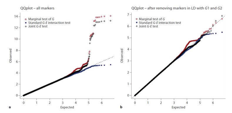
Quantile-quantile plots for a single realization of Y. Trait values have been simulated using the model Y = b_G1G1 + b_G2 + b_EE + ε, where b_G1 = 0.12, b_G2 = 0.05, b_E = 0.05, and b_G2E = 0.1. The genetic inflation factors λ_GC of the marginal test, the standard interaction test and the joint test are equal to 1.019, 1.001, and 1.007 (respectively) for a, and 1.019, 1.001, 1.007 for b.

Table 2.

Example of estimates obtained for G2

Study	Marginal test of G2		Standard test of G2 × E interaction		Joint test of G2 in exposed and unexposed subjects
	all subjects		all subjects		unexposed subjects		exposed subjects
	n	βG2 (SE)	n	βG2E (SE)	n	βG2 (SE)	N	βG2 (SE)
HPFS-CHD	1,311	0.13 (0.04)	1,311	0.12 (0.09)	923	0.09 (0.05)	388	0.21 (0.07)
HPFS-T2D	2,310	0.08 (0.03)	2,310	0.02 (0.07)	1,656	0.07 (0.04)	654	0.09 (0.06)
NHS-CHD	1,145	0.06 (0.04)	1,145	0.12 (0.10)	826	0.03 (0.05)	319	0.15(0.08)
NHS-BRCA	2,285	0.11 (0.03)	2,285	0.23 (0.07)	1,615	0.04 (0.04)	670	0.27 (0.06)
NHS-T2D	3,110	0.06 (0.03)	3,110	0.09 (0.06)	2,247	0.03 (0.03)	863	0.12 (0.05)
Meta-analysis	10,161	0.09 (0.01)	10,161	0.11 (0.03)	7,267	0.05 (0.02)	2,894	0.16 (0.03)
Meta-analysis p value	4.10−8		6.10−4			9.10−10

HPFS = Health Professional Follow-up Study; NHS = Nurse Health Study; CHD = coronary heart disease; BRCA = breast cancer; T2D = type 2 diabetes. Trait values were simulated using the model Y = b_G1G1 + b_G2G2 + b_EE + b_G2EG2 × E + ε, where b_G1 = 0.12, b_G2 = 0.05, b_E = 0.05, and b_G2E = 0.1.

As estimated by simulation, the power of the marginal test for G1 in this situation was greater than 98.91%, and the power of the joint test for G1 was 97.72%. On the other hand, the power to detect G2 using the joint test was 69.92%, while the observed power of the marginal test was 48.81%. The power of the standard test for G2-E interaction was only 0.86%. As expected, since we did not simulate a non-multiplicative joint effect for G1 and E, none of 100,000 realizations of the standard G1-E interaction test were significant at the 5 × 10⁻⁸ level.

Figure 2 shows how the power of these tests changes as more studies are included in a meta-analysis. Generally, power increased non-linearly in the number of studies (reflecting the increase in the total sample size), while the power for any individual study was below 1% for all tests of G1 and G2 (from 0.05% for the marginal test of G2 to 0.002% for the standard G2-E interaction test, and from 0.5% for the marginal test of G1 to 0% for the standard G1-E interaction test). In particular, using fewer than all five available studies led to a concerning decrease of the power for the marginal and joint tests of G2. The removal of one study nearly halved power to detect the Y-G2 association using either of these tests. (The standard G2 × E test had very low power even when using all five studies.) Tests of G2 using less than four studies had less than 10% power. The decrease in power to detect G1 when using fewer studies was smaller than for tests of G2: the power of the marginal test for G1 was 85% when using four studies and 45% when using three studies.

Fig. 2.

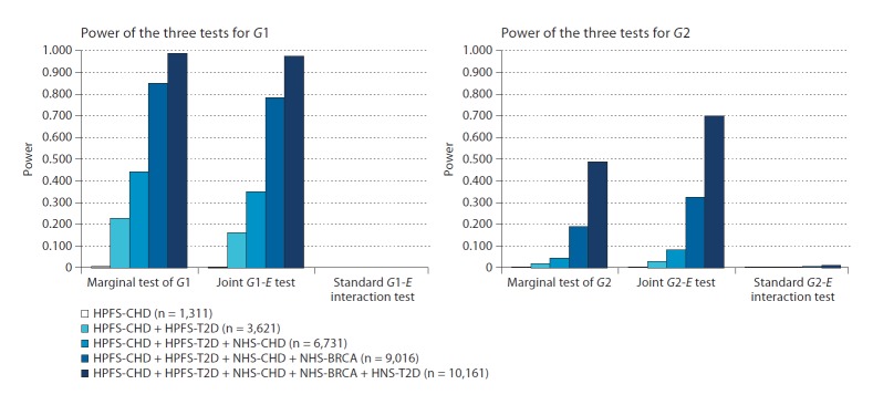
Power of the marginal, joint and interaction tests as more studies are included in the analysis. HPFS: Health Professional Follow-up Study, NHS: Nurse Health Study, CHD: coronary heart disease, BRCA: breast cancer, T2D: type 2 diabetes. Phenotypic data (100,000 realizations of Y) were simulated using the model Y = b_G1G1 + b_G2G2 + b_EE + b_G2E G2 × E, where b_G1 = 0.12, b_G2 = 0.05, b_E = 0.05, and b_G2E = 0.1.

Figure 3 shows the power of the three tests for G2 observed when b_E = 0.05 and varying the values of b_G2 and b_G2E. The power of the joint test to detect G2 is often greater than that of the marginal test. The maximum difference between the power of the joint test and marginal test across these simulated scenarios is 55.46%. The minimum difference, on the other hand, is never more than −7.93%, suggesting that when the joint test has less power than the marginal test its power is not that much smaller. Since the joint test and the standard test of interaction take the environmental effect into account, variation of b_E had no effect on these two tests. However, the power of the marginal test of G1 and G2 decreased for values of b_E over 0.1, and the difference of power of the joint test over the marginal test was increasing in the same proportion. Hence, the joint test of G2 was more powerful than the marginal test of G2 in all situation where b_E was over or equal to 0.5 and the joint test of G1 also was more powerful than the marginal test of G1 when b_E was over 1.0.

Fig. 3.

Power comparison of the marginal tests of G1 and G2, the standard G2-E interaction test and the joint G2-E test. Phenotypic data (1,000 realizations of Y for each point) were simulated using the model Y = b_G1G1 + b_G2G2 + b_EE + b_G2EG2.E + ε, were b_G1, b_E and σ were fixed and respectively equal to 0.12, 0.05 and 1, while we varied b_G2 and b_G2E across a grid defined by b_G2 ∊ {0.01, 0.04, 0.07, 0.1}, and b_G2E ∊ {−0.15 to 0.15 by 0.2}.

Some of the biggest power gains for the joint test come in situations when the main effect of G2 (b_G2) was small and the G2 × E interaction parameter (b_G2E) was large and in the same direction. For example, when b_G2 = 0.04 and b_G2E = 0.13, the power of the joint test was 83%, while the power of the marginal test was 46%. Large gains in power were also observed when the interaction parameter had the opposite sign as the main effect of G2, and consequently the marginal association between G2 and Y was weak. We note that for some of these situations the standard test of interaction has greater power than the marginal test, but it still can have considerably less power than the joint test.

The standard test of gene-environment interaction always showed very low power (under 20% in all simulations), being slightly more powerful than the two other approaches only in some extreme cases, when gene effect was quite low and the interaction effect quite high and opposite to the gene main effect (e.g. b_G2 = 0.04 and b_G2E ≥ −0.13).

Adjusting the marginal tests for G1 or G2 by including a main effect term for the exposure E did not substantially alter the power of these tests: the difference in power between the adjusted and unadjusted tests was quite unchanged when the exposure effect (b_E) was equal or under 0.1. For exposure effect equal or over 1 the power of the unadjusted test for G2 decreases dramatically, while the power of the unadjusted test for G1 decreases in the same range when the exposure effect is higher (i.e. b_E ≥ 2).

Discussion

We have proposed a simple and efficient method for meta-analyses of joint tests of genetic main effect and gene-environment interaction terms. We have shown that this method has an appropriate type I error rate and demonstrated its performance across a wide range of alternative hypotheses via simulation studies. This meta-analytic approach is appropriate for large-scale association studies aimed at discovering markers having low effects on a trait and differing according to an environmental exposure.

Similar to the single-study version of the joint test [5], the meta-analytic test has appropriate type I error rates under the null hypothesis of no association between the tested marker and a phenotype in any stratum defined by the environmental exposure, as long as the marker and the phenotype are uncorrelated in the sampled population [9, 16]. In many situations, including models where the genetic effect in each environmental strata was not null and in the same direction, this meta-analysis of joint test has greater power than either the meta-analysis of standard test for departures from a multiplicative odds ratio model, or the meta-analysis of marginal test for association, making it an attractive test to discover markers which may have been missed by meta-analyses focusing on marginal marker-trait associations (e.g. most meta-analysis of GWAS studies to date).

We have shown that sample sizes far exceeding those of a typical individual GWAS will be needed to reliably detect genes with subtle gene-environment interaction patterns. In the first scenario we simulated, no single study had greater than 1% power to detect a marker whose effect differed across environmental strata (G2). On the other hand, the power of a meta-analysis combining five studies (more than a three-fold increase in sample size relative to the largest individual study) was 58.27 times greater than that of the largest single study; the power of the meta-analysis was greater than 80% for many situations of interest. The large increase in relative power for a smaller increase in relative sample size is due to the non-linear nature of the power curve as a function of sample size. This suggests that meta-analyses incorporating gene-environment interactions may cross a sample-size ‘tipping point’ and identify markers that have gone undetected in individual studies. In the models we simulated, the combined genetic effects of G1 and G2 explained between 0.7 and 1.3% of the total variation in Y, which leads to a high power of the joint and marginal test in the total sample of 10,161 subjects. For a smaller genetic effect, a larger sample size will be required to achieve similar power.

Simulations across a range of genetic main effects and gene-environment interaction effects confirm that in a meta-analysis context, the joint test can be more powerful than either the marginal test of the gene or the standard test of interaction when the genetic effect is weak in one exposure stratum but strong in another, or when the main and interaction effects are in opposite directions (so that the marginal association between the tested marker and the phenotype is weak). However, the latter situation may be of less practical interest since (depending on the context) it may not be biologically plausible; there are few empirical examples of such ‘crossover’ interactions in observational studies [17]. In the range of models we tested, the joint test was often more powerful than the marginal test of the gene, with an absolute gain of power over 50% in the best cases. In situations where the marginal test had better power than the joint test, the difference was small (less than 10% absolute power). The standard test for interaction had low power in all situations we considered; it had slightly greater power than the other two tests only in a few rare, extreme situations. Although we simulated a continuous trait, because the meta-analysis procedure relies on summary parameter estimates (which could be slopes from a linear regression or log odds ratios from a logistic regression), qualitatively similar results should hold for binary disease traits.

Aside from increased power, another potential advantage for the joint test is that it is scale-free. The power and interpretation of tests for the usual gene-environment product term (β_{g e} = 0 in [A]) depend on the link function g(x) [18, 19]. In the context of gene discovery, where the primary goal is establishing associations between markers and a phenotype, no particular scale may have intrinsic interest, and the scale that yields the highest power for the standard interaction test will not be known a priori. For saturated codings of the genetic marker and environmental exposure, the power of the joint test does not depend on the link function for the working model fit to the data [A], but only depends on the true relationship between the marker, exposure and phenotype. However, in situations where departures from additivity on a particular scale are the main interest – for example, when testing for ‘public health interactions’, where the impact of reducing (or increasing) the prevalence of an exposure is larger among genetically susceptible individuals [20] – then the joint test is inappropriate, as it is not a test of interaction per se.

The meta-analysis procedure we propose – [C] – will be useful in typical situations where it is logistically difficult or impossible to share and combine individual-level data. It is easily implemented using standard software for the analysis of GWASs. However, because this particular procedure requires analyses to be conducted within strata of a categorical exposure, in some situations it may lose power relative to analyses that assume a particular form for the interaction term (e.g. ordinal G times continuous E). Moreover, although it does not require that the genetic marker and environmental exposure are independently distributed in the sampled population for validity, it cannot leverage this assumption to increase the power of the individual-study joint tests, as others have proposed [2, 4].

We have sketched a more general approach [B] that uses the variance-covariance matrix for the genetic main effect and gene-environment interaction parameters. This approach could be used to combine evidence from analyses that do not assume a categorical form of the environmental and gene-environment interaction effects, or from analyses that leverage the gene-environment independence assumption. This approach requires straightforward modifications of existing software packages for the analysis and meta-analysis of GWASs. As we were completing this report, we became aware of work by another group that describes the general approach in more detail along with requisite software modifications (unpublished data, Manning et al. [21]). It remains an open question whether a test based on a saturated model for a categorized continuous exposure for both the main effect of the exposure and gene-environment interaction has more power than a test based on a model that simply includes the continuous exposure as a main effect and in a gene-environment product interaction term. Model choice will often be a matter of taste, depending on researchers’ prior beliefs regarding the likely form of any true gene-environment interaction pattern. But the meta-analytic approaches we have outlined here should allow researchers the flexibility to choose the analysis they feel is most appropriate.

References

- 1.Khoury MJ, Wacholder S. Invited commentary: from genome-wide association studies to gene-environment-wide interaction studies – challenges and opportunities. Am J Epidemiol. 2009;169:227–230. doi: 10.1093/aje/kwn351. discussion 234–235. [DOI] [PMC free article] [PubMed] [Google Scholar]
- 2.Chatterjee N, Kalaylioglu Z, Carroll RJ. Exploiting gene-environment independence in family-based case-control studies: increased power for detecting associations, interactions and joint effects. Genet Epidemiol. 2005;28:138–156. doi: 10.1002/gepi.20049. [DOI] [PubMed] [Google Scholar]
- 3.Murcray CE, Lewinger JP, Gauderman WJ. Gene-environment interaction in genome-wide association studies. Am J Epidemiol. 2009;169:219–226. doi: 10.1093/aje/kwn353. [DOI] [PMC free article] [PubMed] [Google Scholar]
- 4.Umbach DM, Weinberg CR. Designing and analysing case-control studies to exploit independence of genotype and exposure. Stat Med. 1997;16:1731–1743. doi: 10.1002/(sici)1097-0258(19970815)16:15<1731::aid-sim595>3.0.co;2-s. [DOI] [PubMed] [Google Scholar]
- 5.Kraft P, Yen YC, Stram DO, Morrison J, Gauderman WJ. Exploiting gene-environment interaction to detect genetic associations. Hum Hered. 2007;63:111–119. doi: 10.1159/000099183. [DOI] [PubMed] [Google Scholar]
- 6.de Bakker PI, Ferreira MA, Jia X, Neale BM, Raychaudhuri S, Voight BF. Practical aspects of imputation-driven meta-analysis of genome-wide association studies. Hum Mol Genet. 2008;17:R122–R128. doi: 10.1093/hmg/ddn288. [DOI] [PMC free article] [PubMed] [Google Scholar]
- 7.Zeggini E, Ioannidis JP. Meta-analysis in genome-wide association studies. Pharmacogenomics. 2009;10:191–201. doi: 10.2217/14622416.10.2.191. [DOI] [PMC free article] [PubMed] [Google Scholar]
- 8.Cornelis MC, Tchetgen Tchetgen EJ, Liang L, Qi L, Chatterjee N, Hu FB, Kraft P: Gene-environment interactions in genome-wide association studies: a comparative study of tests applied to empirical studies of type 2 diabetes. Under review. [DOI] [PMC free article] [PubMed]
- 9.Tchetgen Tchetgen EJ, Kraft P: On the robustness of tests of genetic associations incorporating gene-environment interaction when the environmental exposure is mis-specified. Epidemiology, in press. [DOI] [PMC free article] [PubMed]
- 10.Aulchenko YS, Struchalin MV, van Duijn CM. ProbABEL package for genome-wide association analysis of imputed data. BMC Bioinformatics. 2010;11:134. doi: 10.1186/1471-2105-11-134. [DOI] [PMC free article] [PubMed] [Google Scholar]
- 11.Purcell S, Neale B, Todd-Brown K, Thomas L, Ferreira MA, Bender D, Maller J, Sklar P, de Bakker PI, Daly MJ, Sham PC. PLINK: a tool set for whole-genome association and population-based linkage analyses. Am J Hum Genet. 2007;81:559–575. doi: 10.1086/519795. [DOI] [PMC free article] [PubMed] [Google Scholar]
- 12.van Houwelingen HC, Arends LR, Stijnen T. Advanced methods in meta-analysis: multivariate approach and meta-regression. Stat Med. 2002;21:589–624. doi: 10.1002/sim.1040. [DOI] [PubMed] [Google Scholar]
- 13.Hunter DJ, Kraft P, Jacobs KB, Cox DG, Yeager M, Hankinson SE, Wacholder S, Wang Z, Welch R, Hutchinson A, Wang J, Yu K, Chatterjee N, Orr N, Willett WC, Colditz GA, Ziegler RG, Berg CD, Buys SS, McCarty CA, Feigelson HS, Calle EE, Thun MJ, Hayes RB, Tucker M, Gerhard DS, Fraumeni JF, Jr, Hoover RN, Thomas G, Chanock SJ. A genome-wide association study identifies alleles in FGFR2 associated with risk of sporadic postmenopausal breast cancer. Nat Genet. 2007;39:870–874. doi: 10.1038/ng2075. [DOI] [PMC free article] [PubMed] [Google Scholar]
- 14.Qi L, Cornelis MC, Kraft P, Stanya KJ, Linda Kao WH, Pankow JS, Dupuis J, Florez JC, Fox CS, Pare G, Sun Q, Girman CJ, Laurie CC, Mirel DB, Manolio TA, Chasman DI, Boerwinkle E, Ridker PM, Hunter DJ, Meigs JB, Lee CH, van Dam RM, Hu FB. Genetic variants at 2q24 are associated with susceptibility to type 2 diabetes. Hum Mol Genet. 2010;19:2706–2715. doi: 10.1093/hmg/ddq156. [DOI] [PMC free article] [PubMed] [Google Scholar]
- 15.Li Y, Abecasis GR. Mach 1.0: Rapid haplotype reconstruction and missing genotype inference. Am J Hum Genet. 2006;S79:2290. [Google Scholar]
- 16.Lindstrom S, Yen YC, Spiegelman D, Kraft P. The impact of gene-environment dependence and misclassification in genetic association studies incorporating gene-environment interactions. Hum Hered. 2009;68:171–181. doi: 10.1159/000224637. [DOI] [PMC free article] [PubMed] [Google Scholar]
- 17.Weiss NS. Subgroup-specific associations in the face of overall null results: should we rush in or fear to tread? Cancer Epidemiol Biomarkers Prev. 2008;17:1297–1299. doi: 10.1158/1055-9965.EPI-08-0144. [DOI] [PubMed] [Google Scholar]
- 18.Greenland S. Interactions in epidemiology: relevance, identification, and estimation. Epidemiology. 2009;20:14–17. doi: 10.1097/EDE.0b013e318193e7b5. [DOI] [PubMed] [Google Scholar]
- 19.Kraft P, Hunter DJ. The challenge of assessing gene-environment and gene-gene interactions. In: Khouy MJ, Bedrosian SR, Gwinn M, et al., editors. Human Genome Epidemiology. New York: Oxford University Press; 2010. pp. 165–187. [Google Scholar]
- 20.Siemiatycki J, Thomas DC. Biological models and statistical interactions: an example from multistage carcinogenesis. Int J Epidemiol. 1981;10:383–387. doi: 10.1093/ije/10.4.383. [DOI] [PubMed] [Google Scholar]
- 21.Manning AK, Lavalley M, Liu CT, Rice K, An P, Liu Y, Miljkovic I, Rasmussen-Torvik L, Harris TB, Province MA, Borecki IB, Florez JC, Meigs JB, Cupples LA, Dupuis J. Meta-analysis of gene-environment interaction: joint estimation of SNP and SNP × environment regression coefficients. Genet Epidemiol. 2011;35:11–18. doi: 10.1002/gepi.20546. [DOI] [PMC free article] [PubMed] [Google Scholar]