

Abstract
The inter-site and intra-site variability of system performance of MRI scanners (due to site-dependent and time-variant variations) can have significant adverse effects on the integration of multi-center DTI data. Measurement errors in accuracy and precision of each acquisition determine both the inter-site and intra-site variability. In this study, multiple scans of an identical isotropic diffusion phantom and of the brain of a travelling human volunteer were acquired at MRI scanners from the same vendor and with similar configurations at three sites. We assessed the feasibility of multi-center DTI studies by direct quantification of accuracy and precision of each dataset. Accuracy was quantified via comparison to carefully constructed gold standard datasets while precision (the within-scan variability) was estimated by wild bootstrap analysis. The results from both the phantom and human data suggest that the inter-site variation in system performance, although relatively small among scanners of the same vendor, significantly affects DTI measurement accuracy and precision and therefore the effectiveness for the integration of multi-center DTI measurements. Our results also highlight the value of a DTI-specific phantom in identifying and quantifying measurement errors due to site-dependent variations in the system performance, and its usefulness for quality assurance/quality control in multi-center DTI studies. In addition, we observed that the within-scan variability of each data acquisition, as assessed by wild bootstrap analysis, is of the same magnitude as the inter-site and intra-site variability. We propose that by weighing datasets based on their variability, as evaluated by wild bootstrap analysis, one can improve the quality of the dataset. This approach will provide a more effective integration of datasets from multi-center DTI studies.
Keywords: DTI, multi-center study, precision, accuracy, wild-bootstrap analysis, weighting statistics
INTRODUCTION
Diffusion tensor imaging (DTI) (Basser et al., 1994) is now widely used in the investigation of brain microstructural integrity. DTI-derived parameters, such as fractional anisotropy (FA) and mean diffusivity (MD), are often used to detect subtle changes of tissue diffusion characteristics in the early stage of disease, when no differences are detectable with other traditional MRI methods.
Studies using advanced MRI data, such as DTI, are unique in that the data consist of a large number of image elements (voxels) for each study subject but typically only a relatively small number of subjects can be recruited at a single research site. This motivates the implementation of multi-center studies to acquire an adequate sample size. One common critical question for such a typical multi-center study is whether the data from multiple scanners, either from the same or different vendors, can be integrated into a single dataset, i.e., with negligible site-dependent and time-variant measurement errors associated with the data acquisition.
Measurement error is traditionally attributed to both the accuracy and precision of the measurement (Bevington and Robinson, 1992). Measurement accuracy, δ(X), in general can be quantified by the difference between the true value and the mean value of a large number of repeated measurements of the same parameter X. Precision, σ(X), can be described by the standard deviation from these repeated measurements. The measurement accuracy and precision can affect the power of statistical inference. In the example of a two-group comparison in a single-center study, precision contributes mainly to the spread of data within each group, while the effect of bias in accuracy is more complicated. If the bias of each measurement is constant and time-invariant, in general, the accuracy of the data will not affect the statistical power. However, the bias is more often time-variant (e.g., due to unavoidable drift of scanners over time), and it will increase the standard deviation of the data. The power of statistical comparison will further decrease when data come from scanners of different vendors. Different accuracy levels due to intrinsic system differences will increase the inter-site variability, while the time-variant system performance within each site will result in acquisition-dependent variations of accuracy and precision and consequently increase the intra-site variability.
A multi-center DTI study faces even more challenges. Clinical DTI applications typically use data with low signal-to-noise ratio (SNR), contaminated by physiological noise, artifacts due to field inhomogeneity and eddy currents, and variability due to hardware instability during the lengthy image acquisition (Le Bihan et al, 2006). Except for the physiological noise, all other adverse effects are directly related to the scanner’s performance and, therefore, are usually site-dependent and time-variant. Although all these sources of errors are frequently noted by DTI researchers, no comprehensive quantitative models have been reported to quantify their contributions other than the thermal noise (Pierpaoli and Basser, 1996a; Jones et al., 1999; Hasan et al., 2001; Jones et al., 2004; Poonawalla and Zhou, 2004; Kingsley, 2005).
Recently, nonparametric bootstrap techniques such as wild bootstrap (Whitcher et al., 2008; Jones 2008; Zhu et al., 2009) and residual bootstrap (Chung et al., 2006), have been introduced as robust estimators of precision for DTI measurements. They are particularly applicable to DTI acquisitions within the usual scanning time since only one complete DTI measurement is required. Previous studies (Tofts et al., 2000; Delakis et al., 2004; Nagy et al., 2007) have also demonstrated feasible approaches to quantify bias and to calibrate scanner’s performance by scanning phantoms of isotropic solutions with known diffusivities.
Instead of direct measurement of accuracy and precision, prevailing designs of current multi-center studies rely on analyses of reproducibility and repeatability of data based on pilot studies, in which inter-site (measure for reproducibility) and intra-site (measure for repeatability) variance components are quantitatively analyzed (Zou et al., 2005; Friedman et al, 2008). To quantify measurement errors in multi-center DTI studies, a scan/re-scan theme was adopted in several DTI studies (Pfefferbaum et al., 2003; Marenco et al., 2006; Farrell et al., 2007). These studies provided reliable methods for quantification of data reproducibility and repeatability. However, outcomes from these analyses cannot be used to establish quantitative rejection/acceptance criteria for a given dataset, and there is no approach for utilizing known variability in the accepted data to boost the statistical power. One common approach proposed to deal with the data integration in multi-center studies is to incorporate the site-effect as a random variable into models of advanced variance component analysis (Zou et al., 2005; Friedman et al, 2008). Since the variability due to the site-effect is still included in the model, a relatively large sample size is required with this approach, although site-dependent errors will no longer significantly bias statistical results.
In this study, we directly quantified accuracy and precision of each dataset. For each acquisition, accuracy was estimated using a carefully constructed gold standard dataset while precision (the within-scan variability) was quantified using an optimized wild bootstrap analysis (Zhu et al., 2008). The study was specifically designed to address the following objectives: 1) to investigate inter-site and intra-site differences in DTI measurement accuracy and precision that are due to the site-dependent and time-variant performance of MR scanners in a typical multi-center DTI study;2) to quantitatively compare the within-scan variability of each acquisition (typically not measurable by ANOVA without repeated measurements) with the inter-site and intra-site variance components, and 3) to evaluate the effectiveness of the weighting statistics, which integrates wild bootstrap estimations of the within-scan variability, in reducing the inter-site and intra-site variance. This would improve the quality of the dataset from a multi-center DTI study.
MATERIAL AND METHODS
The effects of site-dependent and time-variant performance of scanners on data integration from multi-center DTI measurements were investigated using multiple scans of identical isotropic DTI phantoms and a human volunteer at three MRI sites of the HIV Neuroimaging consortium (University of Rochester, University of California at San Diego and Stanford University), with scanners from the same vendor and with similar system configurations.
Isotropic Diffusion Phantom and Human Volunteer
A previous study (Tofts et al., 2000) has shown that MD values of three cyclic alkanes (cyclooctane, cycloheptane and cyclohexane) range from 0.5 to 1.4 ×10⁻³mm2/s at 22°C, similar to those of gray matter (GM) and white matter (WM) in human brains (Pierpaoli et al., 1996b). In this study, diffusion phantoms were fabricated at the University of Rochester with cells in a cylindrical polycarbonate container filled with three abovementioned chemicals (Figure 1A). Identical copies of the phantom were delivered to the other two sites. Differences in phantom dimension were well within 1mm. The brain of a healthy volunteer (female, 23 years old) was scanned at three MRI centers. Written consent forms as well as the local institutional review board approval were obtained prior to image acquisitions.
Figure 1.

Measurement precision of phantom data. (A). Photograph (left) and a typical MD map of the isotropic phantom (right). Each phantom contains 16 cells: four cells with cyclohexane (marked by “1”), two with cycloheptane (marked by “2”), four with cyclooctane (marked by “3”) and the rest six cells (marked by “4”) were left empty for anisotropic phantoms in future study. (B)–(C). For each dataset, measurement precision was quantified with two approaches: wild bootstrap analysis using Eq. 1 (with coefficient of variation maps CV(MD) shown in B), and the standard deviation of ADC from repeated measurements (CV(ADC) in C). Maps from acquisitions at two different sites (left and right) are shown. There are clear inter-site differences in precision of DTI measurement (left vs. right), but consistency in the spatial distribution within the phantom was observed between the two approaches (B vs. C). (D). CV(ADCmax_XYZ) map (Eq. 6) quantifies mis-calibration of diffusion weighting gradients along three diffusion gradient directions where the maximum diffusion weighting along physical X, Y, Z directions were applied. (E)–(G). CV(ADCmax_X), CV(ADCmax_Y) and CV(ADCmax_Z) maps (Eq. 5) quantify the repeatability of ADC measurements. Fluctuations in the gradient along physical X axis contribute to the observed measurement variation (indicated by white solid arrows in Figures 1B, 1C and 1E). Site-specific patterns for both mis-calibration and instability of gradients were also observed.
Scan Protocol
For both the phantom and human scans, the following DTI scan protocol (Ferrell et al., 2007) was performed at three sites on GE 1.5T scanners (General Electric, Milwaukee, WI, USA, HDX with 14M software. Gradient type: 8917/HFD-S, RF amplifier type: 1.5T SRFD2): 2D axial DTI using a single-shot spin-echo EPI sequence with dual-spin echoes, TE/TR=75/7000ms, slice thickness=2.5 mm with no gap, data matrix=128×128, FOV=240×240mm, ASSET factor=2, diffusion weighting gradient (DWG) directions=30 with b=1000 s/mm2, and 5 separate b=0s/mm2 images. Within each acquisition, the same protocol was repeated three times and the data of each repeat were saved separately without averaging. A total of ninety diffusion-weighted image (DWI) volumes as well as fifteen non-DWI volumes were generated for each acquisition. The total DTI acquisition time for full brain coverage was 13 minutes.
At each imaging center, a total of five acquisitions of the isotropic DTI phantom were acquired within a period of six weeks with an averaged interval of 8 days between sequential acquisitions. The scanner room temperature at each acquisition was recorded. For human data, two acquisitions within an interval of 24 hours were acquired at each center and a total of six human datasets were obtained.
DTI Image Processing
A custom software tool based on Matlab (The Mathworks, Natick, MA, USA), C++ and various functions in the FSL package (FMRIB Analysis Group, Oxford University, Oxford, UK; Smith et al, 2004) was used for image processing and statistical analysis.
All six human DTI datasets went through three processing steps before applying wild bootstrap resampling and statistical analysis. First, artifacts due to eddy current and subject movement were simultaneously removed using the Eddy Correct tool of FSL. For each dataset, an averaged non-DWI image (AVG_b0) was then generated from a total of 15 non-DWI volumes. Second, among six human DTI datasets, one AVG_b0 image was selected as the reference for co-registrations among different datasets using the FLIRT tool (FMRIB’s Linear Image Registration Tool) of FSL. The resultant transformation matrices were then applied to six datasets to achieve spatial alignments. A super dataset that contained all co-registered acquisitions (90 non-DWI volumes and 540 DWI volumes) was then created as the gold standard for quantifying measurement accuracy of six individual datasets. Disturbances to DWG vectors from image registration were compensated by rotating the original b matrix according to the corresponding rotation matrix from each of the abovementioned two registration steps (Alexander et al., 2000; Rohde et al., 2004). In the final step, diffusion tensors of six original datasets and the super dataset were estimated using a multivariate log-linear fit in which all DWIs and non-DWIs were input as unique measurements without averaging among multiple volumes along the same DWG direction.
For phantom datasets, only corrections for eddy current and motion artifacts within the same acquisition were performed. Accurate positioning at acquisition was achieved with the aid of positioning markers on phantoms (Figure 1A), and in the subsequent quantitative analyses only regions in the center of the cells were considered. Therefore, no co-registration among different acquisitions was performed.
Quantification of Within-Scan Variability with Wild Bootstrap
Wild bootstrap is a non-parametric, data driven procedure for estimating properties of a given statistic with minimum assumptions for the population distribution. From one complete DTI acquisition, it generates a large number (R) of replicas of the original DWI samples (i.e., measured signals) by multiplying fitting residuals from the linear regression process for tensor calculation with an exogenous two-point Rademacher distribution function. Using the “plug-in” principle (Efron et al., 1993), the within-scan variability in DTI-derived parameters, e.g., the precision of MD at each DTI acquisition, σ(MD), or the coefficient of variation for MD, CV(MD), can be estimated from the standard deviation of all wild bootstrap samples, , i.e.
| [1a] |
| [1b] |
Previously reported analytical approaches, including perturbation theory (Anderson 2003; Chang et al., 2007) and error propagation (Poonawalla et al., 2004; Koay et al., 2007) provide efficient and robust quantifications for variance of tensor-derived parameters. However, in human DTI data, the existence of additional sources of uncertainty other than thermal noise, including physiological noise and image artifacts, can violate the Gaussian noise assumption for the first-order perturbation method (Chang et al., 2007). For non-linear regression based error propagation approaches, complex noise structures in DTI can potentially increase the vulnerability to local minimal. This will also increase the inaccuracy from outliers due to artifacts. When compared to these analytical approaches, non-parametric bootstrap resampling techniques have been suggested to be advantageous in the estimation of uncertainty in the presence of artifactual data points (Chang et al., 2007). Furthermore, model-based nonparametric resampling techniques, such as wild bootstrap (Whitcher et al., 2008; Zhu et al., 2008) and residual bootstrap (Chung et al., 2006), are especially applicable to most clinical DTI data acquisitions since they require only one complete DTI measurement to achieve robust estimation of measurement uncertainty. Previous studies (Chung et al., 2006) have shown that wild bootstrap performs equally well when compared to traditional repetition bootstrap in which a minimum of five repeated datasets is necessary. Although underestimation has been reported for bootstrap analysis including wild bootstrap, performance of wild bootstrap analysis for DTI can be improved with optimized implementations (Zhu et al., 2008). Details for implementation of the wild bootstrap analysis in DTI can be found in several previous studies (Chung et al., 2006; Whitcher et al., 2008; Zhu et al., 2008; Jones 2008; Zhu et al., 2009). In this study, an optimized wild bootstrap routine (Zhu et al., 2008) with 1000 bootstrap samples was used after tensor calculation.
Parameters for Measurement Errors of Multi-center DTI Studies at Multiple Levels
For MD and FA of both phantom and human data, five voxelwise quantitative measures were developed for comprehensive analysis of measurement errors. The first two measures (the voxelwise accuracy and precision) quantify intrinsic measurement errors associated with each data acquisition, while the other three measures (the voxelwise within-scan, intra-site and inter-site variance) describe typical variance components present in datasets from multi-center studies. Specifically we assessed, using quantitative measures for MD/FA of cyclohexane in the phantom data as examples when applicable, the following variables:
-
Measurement Accuracy: norm_δ(MD) and norm_δ(FA). The accuracy level was measured as bias values between actual MD/FA from each dataset and the corresponding values from the gold standard dataset constructed for phantom and human data separately. For the isotropic phantom, the gold standard FA value, FAGS, was set to be 0. The scan temperature of each acquisition was recorded and the gold standard MD value, MDGS, was calculated by the mathematical equation for the temperature dependence of diffusivities (Eq. 4 from Tofts et al., 2000). For human DTI, MD/FA values from the super dataset were selected as gold standard values. Voxelwise, normalized bias values, norm_δ(MD), were then calculated as the measure for accuracy using
[2] and similarly for norm_δ (FA).
Measurement Precision (within-scan variability):σ(MD) and σ(FA). The within-scan variability quantified by wild bootstrap analysis (Eq. 1b) reflects the intrinsic uncertainty associated with each DTI acquisition and was consequently selected as the measure for precision.
-
Inter-site Variance Component: σ(MD)inter and σ(FA)inter. It describes the reproducibility of DTI for repeated scans of the same subject or phantom among different sites. For each phantom data, five repeated acquisitions (J=5) were obtained at three sites (I=3) and each acquisition had multiple cells (K=4/2/4 for cyclooctane/cycloheptane/cyclohexane respectively) of the same chemical. For four cells filled with cyclohexane, the four values of MD and FA at the same spatial locations with respect to the center of each cell were treated as four independent observations (i.e. independent samples) of the unknown true value. At each unique spatial location with respect to the cell center, a total of 60 MD values (3 sites × 5 acquisitions/site × 4 cells/acquisition) were used to calculate σ(MD)inter using
[3a] where MDijk represents one MD measurement within the kth cell of the jth acquisition from the ith site, and is the mean value of all sixty MD measurements. represents the mean value of MD of all acquisitions obtained at the ith site. Similar calculations were used for σ(FA)inter.
-
Intra-site Variance Component: σ(MD)intra and σ(FA)intra. It describes the repeatability of DTI measurement for repeated/longitudinal scans of same subject/phantom at the same site. The voxelwise σ(MD)intra/σ(FA)intra was calculated from the sixty MD/FA values using
[3b] where represents the mean value of MD of all the jth acquisition from different sites. Similar calculations were used for σ(FA)intra.
- Within-scan Variance Component: σ(MD)within and σ(FA)within. For phantoms, at each unique spatial location with respect to the cell center, the within-scan variance component was measured as the mean value of sixty wild bootstrap statistics, σ(MD)ijk, using
[3c]
To further improve the robustness of estimation, the corresponding average values of the three voxelwise variance components over a 5×5×5 cubic ROI in the center of a chemical cell were calculated.
For human data, there were six MD values (3 sites×2 acquisitions/site) at each voxel. Different from phantom data in which multiple cells of the same chemical provided multiple independent observations within each acquisition, no multiple observations were available for brain tissue at each spatial location. Instead of Eq. 3, three variance components in human data were calculated voxelwisely using:
| [4a] |
| [4b] |
| [4c] |
where i represents different sites (I=3), and j different longitudinal acquisitions (J=2) within the same site. MDij represents the MD measurement at the jth acquisition from the ith site and σ(MD)ij is the corresponding wild bootstrap estimation. is the mean value of all six MD measurements at each voxel location. Since there were only two acquisitions per site, the intra-site variability in Eq. 4b is the mean value of the absolute difference between two intra-site scans as an approximation.
Inter-Site and Intra-Site Differences in Measurement Accuracy and Precision: Additional Statistical Considerations for Multi-center DTI Studies
For phantom data, the analysis steps for measurement precision of MD of cyclohexane, σ(MD), are presented as an example. An identical process was followed for σ(FA) as well as for accuracy, δ(FA) and δ(MD), of all three chemicals. For every cell, the mean value of σ(MD) over all voxels, , was calculated as the overall precision level for MD at that cell. Five longitudinal phantom datasets were acquired at each site and there were four cyclohexane cells in the phantom, i.e. four independent observations of at each acquisition. Friedman test (a non-parametric test for repeated measurements) was performed with MRI sites (3 levels) and longitudinal acquisitions from the same site (5 levels) selected as two independent variables. The significance level was set to α<0.05.
For human data, Friedman test was applied to 10selected ROIs (Figure 4) representing both major anatomical structures and typical anisotropy levels in human brain. values from ten ROIs of each acquisition were input as multiple observations of the dependent variable. A human white matter atlas (Wakana et al., 2004) was used for locating target WM structures and ROIs.
Figure 4.

Region of interests (ROIs) used for the analysis of human data, are superimposed on the FA map of the super dataset. The eight WM ROIs are: the genu of the corpus callosum (GCC), the body of the corpus callosum (BCC), the splenium of the corpus callosum (SCC), the cingulum (CING), the anterior limb of the internal capsule (ALIC), the posterior limb of the internal capsule (PLIC), the external capsule (EC) and the centrum semiovale (CSO). The two GM ROIs are: the caudate (CAUD) and the putamen (PUT). The corresponding color-coded FA maps are also displayed for reference of anatomical structures.
Cross-validation of Precision Estimation from Wild Bootstrap Analysis and from Isotropic Phantom
As an empirical and data-driven approach, wild bootstrap is intrinsically sensitive to multiple sources of noise, including those caused by fluctuations of hardware, which are usually time-variant. In principle, observed variations among apparent diffusion coefficient (ADC) values of an isotropic solution along different DWG directions effectively provide an overall measurement of variability. For the purpose of cross-validation, measurement precision of MD using wild bootstrap analysis, measured by CV(MD), was compared to the coefficient of variation of ADC values, CV(ADC), calculated from all 90 ADC maps within each DTI dataset, using a similar definition as in Eq. 1.
Two aspects of hardware performance that are unique to DTI acquisitions were further investigated: the repeatability of ADC measurement and the calibration of DWGs. The repeatability of ADC measurement was measured as the standard deviation of ADC values from three repeated measurements along the same DWG direction where the maximum diffusion weighting along physical X,Y,Z axes was applied, using the maximum diffusion weighting along the Z direction:
| [5a] |
| [5b] |
where (ADCmax_Z)i represents one of the three ADC values corresponding to three repeated DWIs along the maximum Z diffusion gradient direction within each phantom acquisition.
Measurement variability due to mis-calibrations of different DWGs was quantified as the standard deviation of all ADC values along three DWG directions where the maximum diffusion weighting along physical X, Y, Z directions were applied,
| [6a] |
| [6b] |
Improving Group Statistics Based on Weighting Statistics and Wild Bootstrap Estimates
Within-scan variability measured via wild bootstrap analysis can be directly integrated with weighting statistics (Bevington and Robinson, 1992; Bland and Kerry, 1998) to improve the overall accuracy and precision of summary statistics from the original data. In data acquisitions of N random samples Xi, different Xi values are usually measured with better or worse precision levels due to the existence of multiple sources for variation, such as site-dependent performance of scanners. Therefore, the traditional mean value will be a less accurate and less precise estimation of the true value. Instead, if the within-scan variability associated with each acquisition of Xi can be quantified, a better estimation can be achieved by calculating the weighted mean of the samples, using
| [7] |
In this equation, each sample is weighted inversely to the variance, , of its measurement, i.e., data with better precision contribute more to the weighted mean, X̄W. The corresponding weighted standard deviation, σW, for the original samples Xi can be expressed as:
| [8] |
This weighted standard deviation, σW, is also an equivalent measure for the precision level of the weighted mean, X̄W. In this study, the wild bootstrap analysis provides a robust estimation of measurement precision, i.e. in Eq. 7. Using both phantom and human data, the effectiveness of the combined weighting statistics and wild bootstrap estimations was evaluated based on two criteria: 1) whether the weighted mean values for FA and MD, and , of multiple acquisitions of the same chemical or the same brain tissue were closer to the gold standard, i.e., improved accuracy of the mean value, and 2) whether the weighted statistics resulted in a smaller standard deviation value, σW, among multiple acquisitions, equivalent to improved precision for the estimation of the mean value.
Using the MD value of cyclohexane as example, for each cell of each phantom dataset, the weighted and non-weighted mean values, ( vs. ), as well as the corresponding standard deviation values (σ(MD)W vs. σ(MD)), over all voxels were calculated. At this point, there were three sets of MD values, and the gold standard values MDGS. Each set had sixty MD values (3 sites × 5 acquisitions/site × 4 values/acquisition). Using Eqs. 3a and 3b, the inter-site and intra-site variability values for and MDGS were then calculated and compared. To quantify the improvement in accuracy of the weighted mean MD value, the bias between and MDGS and the bias between and MDGS were calculated as and . A percent difference (Eq. 9) based on absolute values of and was then calculated for each chemical cell at each acquisition, providing a measure of improvement in accuracy level.
| [9] |
Similarly, the percent difference value for improvement in precision was quantified using
| [10] |
A positive percent difference indicates an improvement inaccuracy or precision from the application of the weighting statistics. For human data, the corresponding percent difference maps using Eqs. 9 and 10 were calculated.
RESULTS
Sources of Measurement Errors and Validation for Wild Bootstrap Estimate: Phantom Study
Figure 1A shows a photograph and a representative MD map of the isotropic DTI phantom. Among all 15 phantom acquisitions, the average scan temperature was 22.3°C (±1.02°C). The average value for MD (unit: ×10−3mm2/s) measurements of three chemicals was 0.55 for cyclooctane, 0.97 for cycloheptane and 1.50 for cyclohexane, in close agreement with their known values. The average SNR values of the non-diffusion weighted image at three sites were 76.46, 78.95 and 75.39 respectively.
The average measurement precision for FA/MD measurements was 0.047/0.036 for cyclooctane, 0.039/0.050 for cycloheptane and 0.039/0.076 for cyclohexane, respectively. Differences in overall precision of MD among the three chemicals reflect intrinsic differences in SNR levels in that cyclohexane has the most attenuated diffusion weighted signal due to its largest MD value among the three chemicals.
Examples of spatial variability in the phantom are shown in Figures 1B–G, where CV(MD) maps (Figure 1B) are compared with the corresponding CV(ADC) maps (Figure 1C). While multiple factors of system performance contribute to variations, issues related to the repeatability of ADC measurement and the calibration of DWGs are illustrated as examples. Between these two sources of variability, mis-calibrations in different DWGs (Figure 1D) are more prominent and contribute largely to the overall variability of ADC signals (Figure 1C) in most chemical cells. Repeatability of ADC measurement along specific DWG directions (Figures 1E to 1G), although being less of a global effect, does contribute significantly to localized ADC variations. For example, when a strong X gradient was applied, large signal fluctuations among three repeated measurements were observed in three cells (indicated by white arrows in Figure 1E).
The consistency between two precision maps, the CV(MD) estimated by wild bootstrap and the CV(ADC) from repeated measurements, indicates the effectiveness of wild bootstrap analysis for measurement precision. Mathematically, MD is the mean value of all ADC values and according to the error propagation theory, there is a relationship of between two estimates where N is the total number of ADC maps and equals to 90 in this study. This explains the approximate 9 to 10 time difference in magnitude between CV(ADC) and CV(MD) in Figure 1.
Due to variability in system performance, positive bias in FA values was observed for all phantom acquisitions. The average bias value of FA measurement was 0.27 for cyclooctane, 0.22 for cycloheptane and 0.20 for cyclohexane. Positive bias in FA observed in this study may also be attributed to the noise effect in isotropic diffusion as reported by a previous study (Pierpaoli et al., 1996a) using Monte Carlo simulations. In contrast, both positive (average +7.0%) and negative (average −2.3%) bias in site-dependent and time-variant patterns of MD measurement were observed, with representative bias maps from three sites shown in Figures 2B–2D.
Figure 2.

Measurement accuracy of phantom data. For each phantom acquisition, measurement accuracy was quantified as the normalized bias (Eq. 2) between the DTI-derived parameters and the corresponding gold standard values. (A). MD maps of individual chemical cells. (B)–(C). The measurement accuracy maps of MD from three acquisitions (B vs. C vs. D) of three different sites (the same datasets and slice locations as those in Figure 1) are displayed as examples. Clear inter-site differences in levels of accuracy were observed.
Measurement Accuracy and Precision: Human Study
The FA map from the super dataset (Figure 3A) shows more anatomical details, a higher contrast-to-noise ratio and an improved level of measurement precision in comparison to the one from a single dataset (Figure 3B). In WM, the FA measurement is more reliable in more anisotropic tissues (Figure 3C). On the other hand, similar precision levels of MD measurement were observed for most WM regions.
Figure 3.

Measurement accuracy and precision inhuman data. (A). A typical FA map from the super dataset (left) is displayed along side with a typical FA map from a single dataset (right). (B). A typical σ(FA) map from the super dataset (left) shows much improved level of precision compared to the corresponding σ(FA) from a single dataset (right). (C). σ(FA) and σ(MD) maps (Eq. 1b) from wild bootstrap analysis of one acquisition represent the measurement precision level of a typical DTI acquisition. (D). normalized bias maps of FA and MD (Eq. 2), with respect to the super dataset, represent the level of measurement accuracy. Contour lines representing the FA value of 0.3 are superimposed on B, C and D for a quick differentiation of white matter and gray matter regions.
As for the accuracy of the DTI measurement (Figure 3D), a positive bias in FA was observed for most brain tissues and this overestimation increased with the decrease of FA values. Negative bias in FA was also observed mostly in GM/WM boundaries where partial volume effects are more dominant. In contrast, negative bias in MD measurement was observed for most tissues. Further investigations of the three eigenvalues revealed an overall underestimation in the smallest eigenvalue for most brain tissues while no obvious bias was observed for the other two eigenvalues.
Inter-Site and Intra-Site Differences in Measurement Accuracy and Precision
For phantom data, there were significant inter-site differences in accuracy of FA in all three chemicals (Friedman test, p < 0.010 for all three chemicals) and inaccuracy of MD of cyclooctane and cyclohexane (p=0.010 and 0.022 respectively) but not for cycloheptane (p=0.33). For precision, there were significant inter-site differences in FA and MD for both cycloheptane and cyclohexane (Friedman test, pFA=0.0076 and 0.0035, pMD=0.041 and 0.015 respectively). In contrast, no significant intra-site differences in either accuracy or precision were detected for any of the chemicals. Results of human data (evaluated from 10 selected ROIs in Figure 4) are illustrated in Figure 5. Similar to phantom results, no significant intra-site differences were detected for either accuracy (pFA=0.16 and pMD =0.067) or precision (pFA≈1.0 and pMD≈1.0), but there were significant inter-site differences in accuracy (pFA<0.010 and pMD<0.0010) and precision (pFA≈0.0010 and pMD<0.0010) of FA and MD.
Figure 5.

Inter-site and intra-site comparisons for measurement accuracy (A, B) and for measurement precision (C, D) in the human data based on 10 selected ROIs. (A) normalized bias of FA, and (B) normalized bias of MD using Eq. 2. (C)Measurement precision (the with-scan variability) of FA and (D) MD using Eq. 1 (unit for σ(MD) is ×10−3mm2/s). The abbreviations have the same definitions as those used in Figure 4.
Within-Scan Variability in Comparison to Inter-Site and Intra-Site Variations
A further comprehensive analysis among the voxelwise inter-site, intra-site and within-scan variability was performed at each spatial location within a 5×5×5 cubic ROI at the center of each chemical cell in the phantom, and at each voxel within the selected ROIs in human data (Figure 4), and the results are presented in Table 1. From both phantom and human data, it is clear that the three sources of variation are of similar magnitude for both FA and MD measurements, except for FA of the phantom where inter-site and intra-site components are on average 4 to 5 times that of the within-scan variability. Site-dependent and time-variant performance of scanners, for example mis-calibrations among different DWGs, may result in different levels of artificial anisotropy in FA measurements of isotropic solutions and contribute to these observed differences in FA measurement
Table 1.
Comparisons of the inter-site, intra-site and within-scan variability in phantom and human data*.
| Voxelwise Variance Components for FA |
Voxelwise Variance Components for MD (×10−3mm2/s) |
|||||
|---|---|---|---|---|---|---|
| Inter-site | Intra-site | Within-scan | Inter-site | Intra-site | Within-scan | |
| Chemicals | ||||||
| Cyclooctane | 0.20 | 0.16 | 0.047 | 0.053 | 0.080 | 0.036 |
| Cycloheptane | 0.18 | 0.13 | 0.039 | 0.088 | 0.087 | 0.050 |
| Cyclohexane | 0.23 | 0.13 | 0.039 | 0.14 | 0.18 | 0.076 |
| Human ROIs | ||||||
| PUT | 0.054 | 0.036 | 0.042 | 0.051 | 0.050 | 0.051 |
| CAUD | 0.040 | 0.032 | 0.034 | 0.037 | 0.026 | 0.038 |
| CSO | 0.043 | 0.039 | 0.036 | 0.034 | 0.032 | 0.041 |
| EC | 0.056 | 0.045 | 0.047 | 0.046 | 0.039 | 0.054 |
| CING | 0.059 | 0.042 | 0.037 | 0.053 | 0.038 | 0.046 |
| ALIC | 0.047 | 0.033 | 0.036 | 0.038 | 0.030 | 0.042 |
| PLIC | 0.066 | 0.050 | 0.039 | 0.093 | 0.074 | 0.052 |
| BCC | 0.042 | 0.039 | 0.034 | 0.041 | 0.043 | 0.039 |
| SCC | 0.044 | 0.043 | 0.047 | 0.060 | 0.069 | 0.071 |
| GCC | 0.057 | 0.058 | 0.047 | 0.046 | 0.038 | 0.058 |
The average values of voxelwise variance components (Eq. 3 for phantom and Eq. 4 for human data) within each selected ROI are listed in the table as estimates for the inter-site, intra-site and within-scan variance components. Using the inter-site variance component of MD of phantom data in the table as the example, it was calculated as the average value of 125 voxelwise [σ(MD)inter]r at a 5×5×5 cubic ROI in the center of each chemical cell, i.e. . The abbreviations for ROIs here have same definitions as those in Figure 4.
Improvement of Group Analyses using a Combination of Weighting Statistics and Wild Bootstrap Estimates
The observed similarity in the magnitude of the three variance components implies that the within-scan variability contributes substantially to the overall inter-site and intra-site variability. Inter-site and intra-site variability can be potentially reduced either with proper control of the within-scan variability or by taking the within-scan variability into consideration when performing statistical analysis. The latter is demonstrated in this study by using weighting statistics to calculate weighted mean values of FA and MD within each chemical cell in the phantom.
For phantom data, the total number of the weighted mean value, either or , was 60 for cyclooctane (5 acquisitions × 3 sites × 4 cells), 30 (5×3×2) for cycloheptane and 60 (5×3×4) for cyclohexane. Among these 150 individual measurements, the accuracy of weighted mean values improved for all FA measurements as indicated by 150 positive %Diff[δ(FA)]values (Figure 6A) and for 117 out of 150 MD measurements (78%) (Figure 6C). For the precision of weighted mean values, 132 out of 150 (88%) FA measurements (Figure 6B) and 143 out of 150 (95%) MD measurements (Figure 6D) showed improved precision in the estimation of weighted means. The average improvement in accuracy was 68% and 48%, and the average improvement for precision was 22% and 25% for FA and MD, respectively. Comparisons of the corresponding inter-site and intra-site variance components calculated from the non-weighted mean value, the weighted mean value and the gold standard value are listed in Table 2. It is clear that the use of weighting statistics adjusts effectively for inter-site and intra-site variance components of both FA and MD measurements for most chemicals. More importantly, the inter-site and intra-site variance components in the weighted dataset are closer to the corresponding gold standard, which indicates an overall improvement of data quality.
Figure 6.

Effectiveness of the weighting statistics combined with wild bootstrap estimation of the within-scan variability in phantom data. Using Eqs. 9 and 10, percent difference values for improvements in accuracy (shown in A for %Diff[δ(FA)] and C for %Diff[δ(MD)]) and for improvements in precision (shown in B for %Diff[σ(FA)] and D for %Diff[σ(MD)]) were calculated respectively for each cell. Positive values indicate improvements with the weighting statistics. It is clear that there are improvements in both accuracy and precision in the majority of the chemical cells when the weighting statistics is used.
Table 2.
Comparisons of the inter-site and intra-site variance components in phantom data: non-weighted, weighted and gold standard*
| Cell-wise Inter-site Variance Component |
Cell-wise Intra-site Variance Component |
||||||
|---|---|---|---|---|---|---|---|
| Non-weighted | Weighted | Gold-standard | Non-weighted | Weighted | Gold-standard | ||
| FA | Cyclooctane | 0.21 | 0.19 | 0 | 0.070 | 0.062 | 0 |
| Cycloheptane | 0.14 | 0.11 | 0 | 0.021 | 0.020 | 0 | |
| Cyclohexane | 0.13 | 0.091 | 0 | 0.040 | 0.037 | 0 | |
| MD (×10−3 mm2/s) | Cyclooctane | 0.10 | 0.031 | 0.030 | 0.092 | 0.063 | 0.040 |
| Cycloheptane | 0.35 | 0.038 | 0.033 | 0.071 | 0.053 | 0.042 | |
| Cyclohexane | 0.081 | 0.062 | 0.060 | 0.14 | 0.11 | 0.078 | |
For human data, %Diff[σ(FA)]maps and %Diff[σ(MD)] maps of locations from two slices are shown as examples in Figure 7. When the weighting statistics was applied, 80.9% and 82.1% of voxels among all brain tissues showed improved precision in FA and MD measurement, respectively. On the two selected slices, significantly increased within-scan variability (Figures 7B and 7C) was observed at regions contaminated by image artifacts along one DWG direction. Using the weighting statistics, significant improvements in precision of FA and MD, indicated as bright red patches in Figures 7D and 7E, were observed at those artifact-contaminated regions with an average percent difference value of 75.0%. For the accuracy of the weighting statistics, 69.7% of the voxels showed improved accuracy in FA measurement while 48.1% voxels had improved accuracy in MD measurement.
Figure 7.
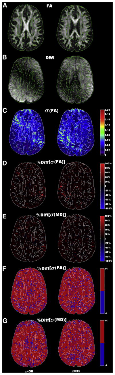
Effectiveness of the weighting statistics combined with wild bootstrap estimation of the within-scan variability in human data. Data from two slice locations (left and right) of one data acquisition are displayed as examples. Contour lines with the FA threshold value of 0.3 are superimposed on each map for a quick differentiation of white matter and gray matter regions. (A). FA maps from locations in two slices. (B). The corresponding DWIs along the diffusion weighting direction where a combination of cardiac pulsation artifacts and signal dropouts due to motion caused signal void within a large region close to the ventricle. (C). The corresponding measurement precision maps, σ(FA), from wild bootstrap analysis, show significant increase of measurement errors in artifact-contaminated region (bright green colors). (D)–(E). Improved precision (warm color) with the weighted mean of six acquisitions, quantified by the percent difference of FA and MD maps, was observed in majority of the brain tissues. Improvements of precision are more prominent in those artifact-contaminated regions (bright red color patches) with an average of 75% improvement. (F)–(G). Corresponding binary maps of %Diff[σ(FA)] and %Diff[σ(MD)] in Figures D and E. The red color represents the voxel locations with improved precision when using weighting statistics, while the blue color represents reduced precision.
DISCUSSION
Multi-center DTI studies inevitably encounter systematic variations due to intrinsic differences among different MRI systems and due to time-dependent variations that occur in the context of a longitudinal study. Pooling data together without quantification and control of the inter-site and intra-site variability will significantly affect statistical analysis of the study which may lead to the need of a much larger sample size to compensate for such variability. A commonly used approach to deal with variability in multi-center studies is to conduct first a pilot study with repeated measurements (both within-site and cross-site) to evaluate feasibility before the larger scale data acquisition takes place. Friedman et al., in the context of a multi-center fMRI study, have taken a different approach in which site-dependent variations are quantified and reduced by either adjusting the acquired data before analysis (Friedman et al., 2006a) or by adjusting variations statistically (Friedman et al., 2006b). With this approach, quantifications of site-dependent variations can be incorporated into statistical analyses to either achieve a better model fitting or to improve the study statistical power.
In this study, we adopted an approach similar to Friedman et al. and quantified data variations in each acquisition directly, in terms of both accuracy and precision level. The ability to evaluate accuracy and precision directly from human DTI data is critical since measurement errors of each acquisition directly determine the inter-site and intra-site variance in the traditional variance component analysis of multi-center studies. Once quantified, the accuracy and precision of each measurement can be used to establish acceptance/rejection criteria for a given dataset. Furthermore, accepted data can be corrected for bias and appropriately weighted to improve data integration.
Our experimental design enables direct quantifications of site-dependent variations attributed to two unique aspects of DTI techniques: repeatability of ADC measurements and calibration of diffusion weighting gradients. All MRI scanners used in this study were from the same vendor with the same hardware/software configurations. In addition, identical isotropic DTI phantoms were used by the participating sites. Without other confounding factors, accuracy and precision of each phantom acquisition directly reflect intrinsic variations of scanners.
The performance of DWGs is the key component in evaluating scanner’s performance of DTI acquisitions. Ideally, the execution of DWG along the same orientation should be stable among repeated measurements and be identical among different DWGs. Several factors, including diffusion gradient execution, eddy current, B0 inhomogeneity, and gradient non-linearity, can cause observed variations among repeated ADC measurements and cause mis-calibrations among DWGs. Any hardware variations, such as the inaccuracy in the amplitude of DWGs, will result in differences between the actual and the prescribed b values. In order to minimize the TE time and maximize the achievable SNR, the maximum amplitude of the diffusion gradient is usually employed (Bernstein et al., 2004). As a result, inaccuracy of the gradient calibration will be more prominent in contrast to traditional MRI techniques. As a consequence of using large DWG amplitudes in DTI, eddy current may affect the actual shape of diffusion gradients, introducing inaccuracy in b values. Although it is now a common practice, also implemented for all scans in this study, to use a twice-refocused spin-echo EPI sequence (Reese et al., 2003) to reduce eddy current artifacts, the inaccuracy in actual b values due to eddy currents cannot be completely compensated for (Le Bihan et al., 2006) and may still contribute to the observed variations in Figure 1. The B0 inhomogeneity, either from imperfect shimming of the magnet or from the localized susceptibility difference within phantoms, results in residual background gradients (Zhong et al., 1991; Le Bihan 1995). The cross-terms between these residual gradients and the actual DWGs could also contribute to the observed variations of ADC maps in Figures 1B and 1D. These effects are orientation-dependent and hard to be modeled without detailed knowledge of specific field mapping at individual gradient directions. In addition, the non-linearity in DWGs may also contribute to the observed spatial distribution of differences between actual and prescribed b values within the phantom. Although the standard quality assurance and quality control (QA/QC) routine was performed regularly in all three participating centers, measurement errors due to all abovementioned issues, did occur as shown by reduced levels of measurement precision (Figure 1B) and accuracy (Figures 2B–2D) of acquired data. More importantly, the observed variations were also site-dependent, which ultimately resulted in significant inter-site differences among multiple acquisitions of both phantom and human data (Figure 5). Evidence from this study clearly demonstrates that even among MRI systems of the same vendor with similar system configurations, site-dependent system performances will significantly affect the quality of acquired DTI datasets that are planned to be integrated.
Using isotropic phantoms in this study also enabled cross-validation between two quantification approaches (repeated measurements and wild bootstrap) for measurement precision. As shown in Figure 1, variations in system performance, especially errors in DWGs, are time-variant and site-specific. When comparing wild bootstrap estimations of CV(MD) to the equivalent estimation of CV(ADC) based on ADC maps, we show that the patterns of spatial distribution of measurement precision within the phantom are nearly identical. The observed consistency between the two quantification approaches provides cross-validations for wild bootstrap analysis. Wild bootstrap analysis can be applied to literally all DTI-derived parameters, including FA and the three eigenvalues, as well as to tissues with different levels of anisotropy. In this study, we applied wild bootstrap analysis to a human dataset as the sole quantification approach for measurement precision. As a data-driven method, wild bootstrap analysis also identified regions with increased measurement errors due to a combination of cardiac pulsation artifacts and signal dropouts due to motion (Figure 7C). Regions with decreased precision in DTI-derived parameters due to physiological noise, such as cardiac pulsation artifacts, were also identified in a recent study (Chung et al., 2010) using residual bootstrap analysis. Taken together, our results and previous studies emphasize that bootstrap analysis can detect various sources of variation in human DTI data. These sources of variation have been largely ignored previously due to the lack of efficient and reliable quantification methods.
To further improve data integration of a multi-center DTI study, we assessed the effectiveness of weighting statistics that incorporates wild bootstrap estimates of precision for individual measurements. Even among MRI scanners from the same vendor with similar configurations, the reliability of each acquisition can be highly site-specific. For example, the within-scan variability level at one site can differ several folds in magnitude from what is observed at another site (Figure 1B, left vs. right). Within one of six DTI acquisitions of the human volunteer, imaging artifacts significantly increased the within-scan variability of FA values in a large region close to the ventricle.
The effectiveness of the weighting statistics was validated in the phantom data and partially validated in the human data. The application of the weighting statistics to phantom FA and MD data resulted in improved accuracy and precision for most weighted mean values (Figure 6). Both inter-site and intra-site variance components based on weighted results were reduced and closer to the corresponding theoretical values (Table 2). The weighting statistics effectively reduced the dispersion of human data FA and MD measurements in most spatial locations. However, the weighting statistics provided mixed results for improvements inaccuracy. There were no substantial improvements inaccuracy with the weighted mean value of MD. This may be partially explained by the limitations of the super dataset used. During the construction of the superset, each of the six DTI datasets was treated equally without taking individual accuracy and precision levels into consideration. This un-weighted approach might have reduced the accuracy level of the superset with respect to the unknown true value for FA and MD. On one hand, the abundance of sample points per direction in the superset maximized the SNR level and consequently improved the robustness of tensor fitting, which resulted in much improved precision of the superset (Figure 3B). On the other hand, as for the accuracy level, the superset could be biased when six datasets from three sites had significantly different bias levels due to intrinsic inter-site differences in system performance. The quality of the superset can be potentially improved with the incorporation of two additional approaches: using robust tensor estimation algorithms and incorporating advanced ground truth estimation algorithms. Robust tensor estimation algorithms like RESTORE (Chang, et al., 2005) adopt iterative nonlinear least squares based regression and exclude identified “outlier” data points from being included for regression. Therefore, they can improve the overall robustness of tensor calculation of each dataset used for construction of the superset. Using maximum-likelihood estimations, advanced bias estimation algorithms (Warfield et al., 2004) can achieve a probabilistic estimate of the true bias level and obtain the performance evaluation of bias estimations for each scan simultaneously. Implementing RESTORE and developing bias estimation for multi-center DTI studies merit a future study.
A larger number of subjects necessary for biodiversity and demographic characteristics for a given disease process can be obtained more efficiently in a multi-center study (Friedman et al., 2008). With broadening applications of DTI, it becomes increasingly important to address the issue of intra-site and inter-site variability in data acquisition. While remaining an active research topic, several general guidelines for conducting multi-center DTI studies have emerged within the research community (Collins 2005; Pierpaoli 2005; Pierpaoli 2009), including optimization of DTI protocols, standardization of scanners and acquisition procedure, centralization of data processing and implementation of reliable QA/QC procedures. Following these guidelines, we were able to design a multi-center study of isotropic diffusion phantoms and a travelling human volunteer. We were able to quantitatively evaluate the within-scan, intra-site and inter-site variance components that ultimately determine the quality of data to be pooled for analyses.
We believe that two results in this study can further facilitate better practices in multi-center DTI studies. First, although we used isotropic DTI phantoms in this study mainly to quantify three variance components associated with a typical multi-center DTI, the isotropic phantom scan can be used as part of a QA/QC procedure within multi-center DTI studies to monitor the system performance and to identify possible sources of bias on a regular basis. Even though anisotropic DTI phantoms (Yanasak et al., 2008; Fieremans et al., 2008), which are under active and extensive studies, can potentially characterize tissue diffusion anisotropy, diffusion characteristics of isotropic phantoms have been well characterized (Tofts et al., 2000), and more importantly, robust quantifications of hardware fluctuations/variations can be achieved with measurements of variations of an isotropic phantom.
A previous study by Delakis et al (2004) has shown that evaluations of longitudinal ADC measurements based on two isotropic solutions (CuSO4 and sucrose) can help to identify orientation-dependent variations with diffusion gradients of their MRI scanner. In a more recent study (Nagy et al., 2007), a scaling factor was derived from the bias level of a uniform water phantom to calibrate the gradient system and the robustness of tensor calculation was significantly improved after calibrations.
To achieve more comprehensive QA/QC protocols with diffusion-specific phantoms, further improvements in phantom design are needed in future studies. Three cyclic alkanes were selected in this study due to high repeatability of diffusivity measurements (Tofts et al., 2000). However, these chemicals are expensive and hazardous to handle due to their toxic and evaporative characteristics. They may not be suitable for the QA/QC routine in a clinical imaging facility. A recent study (Pierpaoli et al., 2009) has shown that polyvinylpyrrolidone (PVP) solutions with different concentrations have similar diffusion properties to those of the normal brain tissue. PVP is stable, inexpensive and without known toxicity and likely a good alternative for diffusion phantom material.
The second contribution of this study to multi-center DTI studies is to implement weighting statistics based on empirical bootstrap analysis. Even though robust tensor estimation algorithms, such as RESTORE (Chang, et al., 2005), have been employed to improve the robustness of tensor estimation for each individual dataset and they have been proven useful in regions contaminated by image artifacts (Walker et al., 2010), most of these methods may not distinguish thermal-noise induced errors from artifact induced errors (Chang, et al., 2005). Therefore, data points satisfying the acceptance criteria might still be contaminated by artifacts. Without accounting for different uncertainty levels, the overall statistical power of the combined multi-center dataset is not maximal. For the weighting statistics proposed in this study, uncertainty level associated with tensor-derived parameters is quantified by wild bootstrap analysis. Therefore, when grouping data with different uncertainty levels from different centers, the contribution of each dataset to the final statistical analysis can be weighted according to the corresponding uncertainty level. Datasets with larger uncertainty values, indicating less reliable measurements during data acquisition, will contribute less to the final statistical analysis and, therefore, weighting statistics will improve the overall statistical power. With the requirement of only one complete DTI dataset, the weighting statistics with wild bootstrap analysis can be easily implemented in most data processing procedures of multi-center DTI studies.
Results from both phantom and human data in this study have shown that the three variance components (within-scan, intra-site and inter-site) have similar amplitudes for a typical multi-center DTI study using scanners from the same vendor with similar configurations. This implies that if no additional approaches were taken, the overall variability for the data from a multi-center study will potentially increase substantially in comparison to a single-center study with the same number of subjects. Therefore, we believe that when designing a multi-center DTI study, it is useful to combine both robust tensor estimation algorithms and weighting statistics in order to not only reduce the within-scan variability of each dataset (by using robust algorithms) but also reduce the intra-site and inter-site variability (by implementing weighting statistics). Although, we implemented wild bootstrap analysis only for tensor calculation with least-square linear regression, it can be integrated with robust tensor estimation algorithms, such as RESTORE, to estimate measurement uncertainty. This merits a future study.
CONCLUSIONS
Consistent results from both phantom and human data show that inter-site variations, although small among scanners of the same vendor, will affect the integration of multi-center DTI measurements. Results from this study also indicate that with a DTI-specific phantom, such as the isotropic phantom applied in this study, it is possible to identify and quantify measurement errors due to site-dependent variations in system performances. We have also shown the usefulness of wild bootstrap analysis in estimating the within-scan variability with each dataset acquisition.
The overreaching conclusion from this study is that, complementary to the current general guidelines for multi-center DTI studies, it is important to develop standardized DTI-specific QA/QC routines to calibrate system performance using isotropic phantoms at participating centers. It is also beneficial to integrate weighting statistics with wild bootstrap analysis into the centralized data processing pipeline to further improve the quality of the data collected and thus the statistical power of the study.
Acknowledgments
The authors appreciate the thoughtful suggestions from anonymous reviewers. This study is a cooperative effort from three imaging centers within the HIV Neuroimaging consortium.
This project was supported by NIH RO1-NS036524.
Footnotes
Publisher's Disclaimer: This is a PDF file of an unedited manuscript that has been accepted for publication. As a service to our customers we are providing this early version of the manuscript. The manuscript will undergo copyediting, typesetting, and review of the resulting proof before it is published in its final citable form. Please note that during the production process errors may be discovered which could affect the content, and all legal disclaimers that apply to the journal pertain.
References
- Anderson AW. Theoretical analysis of the effects of noise on diffusion tensor imaging. Magn Reson Med. 2001;46:1174–1188. doi: 10.1002/mrm.1315. [DOI] [PubMed] [Google Scholar]
- Basser PJ, Mattiello J, Le Bihan D. MR diffusion tensor spectroscopy and imaging. Biophys J. 1994;66:259–267. doi: 10.1016/S0006-3495(94)80775-1. [DOI] [PMC free article] [PubMed] [Google Scholar]
- Bernstein MA, King KF, Zhou XJ. Handbook of MRI pulse sequences. Academic Press, Inc; 2004. pp. 274–280. [Google Scholar]
- Bevington PR, Robinson DK. Data reduction and error analysis for the physical sciences. New York: McGraw-Hill, Inc; 1992. pp. 58–63. [Google Scholar]
- Bland JM, Kerry SM. Weighted Comparison of means. BMJ. 1998;316:129. doi: 10.1136/bmj.316.7125.129. [DOI] [PMC free article] [PubMed] [Google Scholar]
- Chang LC, Koay CG, Pierpaoli C, Basser PJ. Variance of estimated DTI-derived parameters via first-order perturbation methods. Magn Reson Med. 2007;57:141–149. doi: 10.1002/mrm.21111. (Erratum: Magn Reson Med 2008, 59, 946) [DOI] [PubMed] [Google Scholar]
- Chung S, Lu Y, Henry RG. Comparison of bootstrap approaches for estimation of uncertainties of DTI parameters. Neuroimage. 2006;33:531–541. doi: 10.1016/j.neuroimage.2006.07.001. [DOI] [PubMed] [Google Scholar]
- Chung S, Courcot B, Sdika M, Moffat K, Rae C, Henry RG. Bootstrap quantification of cardiac pulsation artifact in DTI. Neuroimage. 2010;49:631–640. doi: 10.1016/j.neuroimage.2009.06.067. [DOI] [PubMed] [Google Scholar]
- Collins DL. What quality control procedures should we be adopting for single-and multi-center studies?. And what should the minimal reporting requirements be? ISMRM Workshop on Methods for Quantitative Diffusion MRI of Human Brain; Lake Louise, Canada. 2005. [Google Scholar]
- Delakis I, Moore EM, Leac MO, Wilde JPD. Developing a quality control protocol for diffusion imaging on a clinical MRI system. Phys Med Biol. 2004;49:1409–1422. doi: 10.1088/0031-9155/49/8/003. [DOI] [PubMed] [Google Scholar]
- Efron B, Tibshirani R. An introduction to the bootstrap. New York: Chapman and Hall; 1993. p. 436. [Google Scholar]
- Farrell JAD, Landman BA, Jones CK, Smith SA, Prince JL, van Zijl PCM, Mori S. Effects of signal-to-noise ratio on the accuracy and reproducibility of diffusion tensor imaging derived fractional anisotropy, mean diffusivity, and principal eigenvector measurement at 1.5T. J Magn Reson Imaging. 2007;26:756–767. doi: 10.1002/jmri.21053. [DOI] [PMC free article] [PubMed] [Google Scholar]
- Fieremans E, De Deene Y, Delputte S, Ozdemir MS, D’Asseler Y, Vlassenbroeck J, Deblaere K, Achten E, Lemahieu I. Simulation and experimental verification of the diffusion in an anisotropic fiber phantom. J Magn Reson. 2008;190:189–99. doi: 10.1016/j.jmr.2007.10.014. [DOI] [PubMed] [Google Scholar]
- Friedman L, Glover GH, Krenz D, Magnotta V, FIRST BIRN. Reducing Scanner-to-scanner variability of activation in a multi-center fMRI study: role of smoothness equalization. Neuroimage. 2006a;32:1656–1668. doi: 10.1016/j.neuroimage.2006.03.062. [DOI] [PubMed] [Google Scholar]
- Friedman L, Glover GH the FRIRN consortium. Reducing interscanner variability of activation in a multicenter fMRI study: Controlling for signal-to-fluctuation-noise-ratio (SFNR) differences. Neuroimage. 2006b;33:471–481. doi: 10.1016/j.neuroimage.2006.07.012. [DOI] [PubMed] [Google Scholar]
- Friedman L, Stern H, Brown GG, MAthalon DH, Turner J, Glover GH, Gollub RL, Lauriello J, Lim KO, Cannon T, Greve DN, Bockholt HJ, Belger A, Mueller B, Doty MJ, He J, Wells W, Smyth P, Pieper S, Kim S, Kubicki M, Vangel M, Potkin SG. Test-retest and between-site reliability in a multicenter fMRI study. Human Brain Mapping. 2008;29:958–972. doi: 10.1002/hbm.20440. [DOI] [PMC free article] [PubMed] [Google Scholar]
- Koay CG, Chang LC, Pierpaoli C, Basser PJ. Error propagation framework for diffusion tensor imaging via diffusion tensor representations. IEEE Tran Med Imaging. 2007;26:1017–1034. doi: 10.1109/TMI.2007.897415. (Erratum:2007, IEEE Trans Med Imaging 26, 1424) [DOI] [PubMed] [Google Scholar]
- Hasan KM, Parker DL, Alexander AL. Comparison of gradient encoding schemes for diffusion-tensor MRI. J Magn Reson Imaging. 2001;113:769–780. doi: 10.1002/jmri.1107. [DOI] [PubMed] [Google Scholar]
- Jones DK, Horsfield MA, Simmons A. Optimal strategies for measuring diffusion in anisotropic system by magnetic resonance imaging. Magn Reson Med. 1999;42:515–525. [PubMed] [Google Scholar]
- Jones DK. The effect of gradient sampling schemes on measures derived from diffusion tensor MRI: a Monte Carlo study. Magn Reson Med. 2004;51:807–815. doi: 10.1002/mrm.20033. [DOI] [PubMed] [Google Scholar]
- Jones DK. Tractography gone wild: probabilistic fiber tracking using the wild bootstrap with diffusion tensor MRI. IEEE Trans Med Imaging. 2008;27:1268–1274. doi: 10.1109/TMI.2008.922191. [DOI] [PubMed] [Google Scholar]
- Kingsley PB. Optimization of DTI acquisition parameters. Proceedings of the 13th Annual Meeting of ISMRM; Miami, FL, USA. 2005. abstract 1294. [Google Scholar]
- Le Bihan D. Diffusion NMR imaging with spin echoes. In: Le Bihan D, editor. Diffusion and Perfusion Magnetic Resonance Imaging. New York: Raven Press Ltd; 1995. pp. 19–27. [Google Scholar]
- Le Bihan D, Poupon C, Amadon A, Lethimonnier F. Artifacts and pitfalls in diffusion MRI. J Magn Reson Imaging. 2006;24:478–488. doi: 10.1002/jmri.20683. [DOI] [PubMed] [Google Scholar]
- Marenco S, Rawlings R, Rohde GK, Barnett AS, Honea RA, Pierpaoli C, Weinberger DR. Regional distribution of measurement error in diffusion tensor imaging. Psychiatry Res. 2006;147:69–79. doi: 10.1016/j.pscychresns.2006.01.008. [DOI] [PMC free article] [PubMed] [Google Scholar]
- Nagy Z, Weishopf N, Alexander DC, Deichmann R. A method for improving the performance of gradient systems for diffusion-weighted MRI. Magn Reson Med. 2007;58:763–768. doi: 10.1002/mrm.21379. [DOI] [PMC free article] [PubMed] [Google Scholar]
- Pfefferbaum A, Adalsteinsson E, Sullivan EV. Replicability of diffusion tensor imaging measurements of fractional anisotropy and trace in brain. J Magn Reson Imaging. 2003;18:427–433. doi: 10.1002/jmri.10377. [DOI] [PubMed] [Google Scholar]
- Pierpaoli C, Basser PJ. Toward a quantitative measurement of diffusion anisotropy. Magn Reson Med. 1996a;36:893–906. doi: 10.1002/mrm.1910360612. [DOI] [PubMed] [Google Scholar]
- Pierpaoli C, Jezzard P, Basser PJ, Barnett A, Di Chiro G. Diffusion tensor MR imaging of the human brain. Radiology. 1996b;201:637–648. doi: 10.1148/radiology.201.3.8939209. [DOI] [PubMed] [Google Scholar]
- Pierpaoli C. How does physiological noise contaminate diffusion data, and what can we do about it? (Subject motion, cardiac pulsation). ISMRM Workshop on Methods for Quantitative Diffusion MRI of Human Brain; Lake Louise, Canada. 2005. [Google Scholar]
- Pierpaoli C, Sarlls JE, Nevo U, Basser PJ, Horkay F. Polyvinylpyrrolidone (PVP) water solutions as isotropic phantoms for diffusion MRI studies. Proceedings of the 17th Annual Meeting of ISMRM; Honolulu, HI, USA. 2009. abstract 1414. [Google Scholar]
- Pierpaoli C. How to do a DTI multi-center neuroimaging study. Weekday educational course of the 17th Annual Meeting of ISMRM; Honolulu, HI, USA. 2009. [Google Scholar]
- Poonawalla AH, Zhou XJ. Analytical Error Propagation in Diffusion Anisotropy Calculations. J Magn Reson Imaging. 2004;19:489–498. doi: 10.1002/jmri.20020. [DOI] [PubMed] [Google Scholar]
- Reese TG, Heid O, Weisskoff RM, Wedeen VJ. Reduction of eddy-current-induced distortion in diffusion MRI using a twice-refocused spin echo. Magn Reson Med. 2003;49:177–182. doi: 10.1002/mrm.10308. [DOI] [PubMed] [Google Scholar]
- Rohde GK, Barnett AS, Basser PJ, Marenco S, Pierpaoli C. Comprehensive approach for correction of motion and distortion in diffusion-weighted MRI. Magn Reson Med. 2004;51:103–114. doi: 10.1002/mrm.10677. [DOI] [PubMed] [Google Scholar]
- Smith SM, Jenkinson M, Woolrich MW, Beckmann CF, Behrens TEJ, Johansen-Berg H, Bannister PR, De Luca M, Drobnjak I, Flitney DE, Niazy R, Saunders J, Vickers J, Zhang Y, De Stefano N, Brady JM, Matthews PM. Advances in functional and structural MR image analysis and implementation as FSL. NeuroImage. 2004;23:208–219. doi: 10.1016/j.neuroimage.2004.07.051. [DOI] [PubMed] [Google Scholar]
- Tofts PS, Lloyd D, Clark CA, Barker GJ, Parker GJM, McConville P, Baldock C, Pope JM. Test liquids for quantitative MRI measurements of self-diffusion coefficient in vivo. Magn Reson Med. 2000;43:368–374. doi: 10.1002/(sici)1522-2594(200003)43:3<368::aid-mrm8>3.0.co;2-b. [DOI] [PubMed] [Google Scholar]
- Wakana S, Jiang HY, Nagae-Poetscher LM, van Zijl PCM, Mori S. Fiber tract-based atlas of human white matter anatomy. Radiology. 2004;230:77–87. doi: 10.1148/radiol.2301021640. [DOI] [PubMed] [Google Scholar]
- Walker L, Chang LC, Koay CG, Sharma N, Cohen L, Verma R, Pierpaoli C. Effects of physiological noise in population analysis of diffusion tensor MRI data. Neuroimage. 2010 doi: 10.1016/j.neuroimage.2010.08.048. [DOI] [PMC free article] [PubMed] [Google Scholar]
- Warfield SK, Zou KH, Wells WM. Simultaneous truth and performance level estimation (STAPLE): an algorithm for the validation of image segmentation. IEEE Trans Med Imaging. 2004;23:903–921. doi: 10.1109/TMI.2004.828354. [DOI] [PMC free article] [PubMed] [Google Scholar]
- Whitcher B, Tuch DS, Wisco JJ, Sorenson AG, Wang L. Using the wild bootstrap to quantify uncertainty in DTI. Human Brain Mapping. 2008;29:346–362. doi: 10.1002/hbm.20395. [DOI] [PMC free article] [PubMed] [Google Scholar]
- Yanasak NE, Jerry DA, Hu TCC. An empirical characterization of the quality of DTI data and the efficacy of dyadic sorting. Magn Reson Imaging. 2008;26:122–132. doi: 10.1016/j.mri.2007.05.006. [DOI] [PubMed] [Google Scholar]
- Zhong JH, Kennan RP, Gore JC. Effects of susceptibility variations on NMR measurements of diffusion. J Magn Reson. 1991;95:267–280. [Google Scholar]
- Zhu T, Liu X, Connelly PR, Zhong J. An optimized wild bootstrap method for evaluation of measurement uncertainties of DTI-derived parameters in human brain. Neuroimage. 2008;40:1144–1156. doi: 10.1016/j.neuroimage.2008.01.016. [DOI] [PubMed] [Google Scholar]
- Zhu T, Liu X, Gaugh M, Connelly P, Ni H, Ekholm S, Schifitto G, Zhong J. Evaluation of measurement uncertainties in human DTI-derived parameters and optimization of clinical DTI protocols with a wild bootstrap analysis. J Magn Reson Imaging. 2009;29:422–435. doi: 10.1002/jmri.21647. [DOI] [PubMed] [Google Scholar]
- Zou KH, Greve DH, Wang M, Pieper SD, Warfield SK, White NS, Manandhar S, Brown GG, Vangel MG, Kikinis R, Wells WM., III Reproducibility of functional MR imaging: preliminary results of prospective multi-institutional study performed by biomedical informatics research network. Radiology. 2005;237:781–789. doi: 10.1148/radiol.2373041630. [DOI] [PMC free article] [PubMed] [Google Scholar]