Helmholtz-pair transmit coil with integrated receive array for high-resolution MRI of trabecular bone in the distal tibia at 7 T

Abstract

A Helmholtz-pair local transmit RF coil with an integrated four-element receive array RF coil and foot immobilization platform was designed and constructed for imaging the distal tibia in a whole-body 7 T MRI scanner. Simulations and measurements of the B₁ field distribution of the transmit coil are described, along with SAR considerations for operation at 7 T. Results of imaging the trabecular bone of three volunteers at 1.5 T, 3 T and 7 T are presented, using identical 1.5 T and 3 T versions of the 7 T four-element receive array. The spatially registered images reveal improved visibility for individual trabeculae and show average gains in SNR of 2.8x and 4.9x for imaging at 7 T compared to 3 T and 1.5 T, respectively. The results thus display an approximately linear dependence of SNR with field strength and enable the practical utility of 7 T scanners for micro-MRI of trabecular bone.

1. Introduction

With the advent of whole-body 7 T research scanners, and with trends to even higher field strengths, there have been hopes of translating MRI technology to these ultra-high field strengths in order to capitalize on expected SNR increases. Some groups have had preliminary success with musculoskeletal imaging of cartilage and trabecular bone at 7 T (1–3). However, the speed of the transition to ultra-high field has been hindered by technical challenges related to increased radio frequency (RF) field inhomogeneity and power deposition within tissue, with corresponding non-uniform flip angles and regions of high specific absorption rate (SAR). Furthermore, the lack of a transmit body coil for these scanners has meant that the full potential of receive array coils has yet to be realized. Recent developments in transmit array technology have shown promise for various applications at ultra-high field (4,5), allowing for spatial tailoring of the ${\text{B}}_1^{+}$ transmit field, but requiring multiple RF transmit channels which are not available on most scanners. Hence single channel approaches still have wide applicability, particularly for imaging of the extremities as is common in musculoskeletal studies.

A case in point is the study of osteoporosis, a systemic disease involving loss of trabecular bone leading to greater risk of bone fractures. It has been shown that the quality of the trabecular network is an important determinant of a bone’s strength and resistance to fracture (6). While fractures in the vertebrae and in the hip are considered to have the highest associated morbidity, surrogate sites in the appendicular skeleton can be used to assess the quality of the trabecular bone network and to monitor changes in the micro-architecture serially. Such measurements in the distal radius and tibia by micro-MRI (7–9) can provide high-resolution three-dimensional images of trabecular bone non-invasively, referred to in the authors’ lab as a virtual bone biopsy (VBB), and these image data, combined with advanced algorithms for quantifying the trabecular network topology, have proven to have strong predictive power for fracture risk and treatment efficacy of metabolic bone disease in humans (10–13).

The accuracy of quantitative methods such as the VBB can be greatly benefited by the increase in SNR accessible at higher fields. In order to enable VBB MRI methods at 7 T, we therefore have implemented a local transmit RF coil for exciting ¹H spins in the distal tibia (14). The design and construction of this transmit coil, along with a custom designed four-element receive array coil and immobilization platform, are described here and results are shown of trabecular bone micro-MRI in volunteers. Comparison also is made with matched results at 1.5 T and at 3 T using identically designed four-element receive coils (Insight MRI, Inc., Worcester, MA) to estimate the SNR dependence on field strength for VBB micro-MRI methods.

2. Materials and methods

2.1. Coil design and construction

The integrated transmit-receive tibia RF coil was designed to interface with a Siemens 7 T whole-body (60 cm bore) MRI scanner (Siemens Medical Systems, Erlangen, Germany). The scanner operates at 297.2 MHz for ¹H imaging, is equipped with gradients of maximum amplitude and slew rate 40 mT/m and 200 T/m/s, and has a single RF transmit channel but has no RF body coil. Design stages for the tibia coil included simulations, prototype construction, and final assembly, as illustrated in Fig. 1. Circuit details are given in the Appendix. Simulation of RF currents and fields in three dimensions was based on a Method of Moments calculation (15,16) in order to optimize the unloaded coil geometry. The unloaded configuration is useful for relative comparisons even at frequencies as high as 300 MHz, with the caveat that simulated currents and fields are perturbed by the presence of a load (e.g., an ankle). Therefore, feasibility of the design was confirmed by constructing a prototype that could be tuned and matched while loaded by a human ankle.

Fig. 1.

Coil design stages: simulations, construction, and final assembly. A) RF current and ${\text{B}}_1^{+}$ field simulations for a shielded Helmholtz-pair transmit coil, estimating ${\text{B}}_1^{+}$ field deviation over a (6 cm)³ volume. B) Helmholtz-pair without and with its enclosure and with slotted RF shield visible. C) Four-element receive array simulated ${\text{B}}_1^{-}$ field and photo with cover removed showing locations of on-board preamps. D) Completed transmit-receive coil assembly with support for the non-imaged foot.

The primary design plan for the transmit coil was a Helmholtz-pair with a 10-inch (25.4 cm) loop diameter. This is the maximum size that will allow a patient’s leg to be both at the magnet isocenter and at the center of the Helmholtz loops, since the distance from isocenter to the surface of the patient table is about 15 cm. Thus the coil could be placed at isocenter and oriented with its loop axis orthogonal to the static field B₀ To avoid current phase variation along the length of the loops, which can occur at 300 MHz due to the relatively short wavelength in copper (λ/4 < 25 cm) compared to the size of the coil, series tuning capacitors of equal value were used to break up the current path along each loop. For this, 12 equidistant breaks initially were chosen and tuning and matching capacitor values were varied in order to minimize $\mathrm{\Delta }{\text{B}}_1^{+}$, i.e., the deviation of the forward-rotating transmit field ${\text{B}}_1^{+}$ within a (6 cm)³ region between the two loops from its value at the center (Fig. 1A). A target of $\mathrm{\Delta }{\text{B}}_1^{+}\le 5\%$ was specified. An additional optimization parameter used was the deviation of current in the tuning capacitors around the loops, defined as Δi = (i_max − i_min)/(i_max + i_min), where i_max and i_min are maximum and minimum currents in the capacitors. At high frequency, capacitors along the loops, even if equal-valued, can carry non-equal currents due to current phase variation. However, for minimum $\mathrm{\Delta }{\text{B}}_1^{+}$, ideally Δi should be zero.

The Helmholtz-pair coil without and with its plastic enclosure is shown in Fig. 1B, with the slotted RF shield visible. The shield was slotted to reduce possible effects of gradient-induced eddy currents. For signal reception, a decoupled four-element receive array coil (Fig. 1C) was chosen to be integrated with the Helmholtz pair in order to maximize SNR, based on high quality images that had been obtained with an identical 3 T version of the four-element receive array (17). The receive coil was constructed with 50×58 mm² rectangular overlapping elements, having on-board preamplifiers and both active and passive diode-based detuning strategies (see Appendix). The 1.5 T and 3 T versions of this four-element receive coil had been constructed with identical dimensions and electronics as the 7 T version, but tuned to 63.6 MHz and 123.3 MHz, respectively. Furthermore, the cables for both transmit and receive coils included baluns to prevent large shield voltages. The final transmit-receive assembly (Fig. 1D) was compact and provided intrinsic immobilization for the foot by means of an integrated footrest. An additional support for the non-imaged foot was constructed from Delrin plastic. This was designed to fit securely at the side of the Helmholtz coil to provide equal elevation and immobilization for both feet, which were secured using Velcro straps. Also visible in Fig. 1D are plastic rods with red flags that attach to variable capacitors located at the top of each loop for the purpose of fine tuning the transmit coil resonance frequency.

2.2. SAR estimation

Simulations

At 7 T, spatial distributions of the RF electric and magnetic fields within tissue are difficult to predict, and local hot spots of RF power absorption can occur. To assure safe operation of the transmit coil for in vivo imaging and yet avoid unnecessary restriction on its use, the peak or maximum local (i.e., within 10 g tissue) SAR generated per unit of applied RF power had to be determined. This is set in the scanner’s software by the coil-specific K parameter. For a given pulse sequence and transmit coil, the scanner multiplies the required RF power (in Watts) by K (in kg⁻¹) in order to compute the peak SAR (in W/kg) that will be generated. The pulse sequence will run only if peak SAR is less than or equal to the IEC guideline for non-significant risk (≤ 100% SAR). Therefore to determine K, SAR distributions generated by the Helmholtz coil were simulated for a human ankle and for ankle-sized phantoms using a full-wave, 3D, electromagnetic analysis software package based on the finite difference time domain method (XFDTD version 6.5, Remcom, Inc., State College, PA). The XFDTD software also provided maps of B₁ and electric field. The simulations were corroborated by flip angle mapping and supplemented by temperature measurements in a real phantom in order to arrive at a final value for K, as described below.

An accurate mesh model of the Helmholtz coil (1×1×1 mm³ element size) was created in XFDTD by importing a 3D CAD file that had been made in Solid Works (Dassault Systèmes Solid Works Corp., Concord, MA) during coil design. Capacitor gaps were treated as passive ports of 6 pF capacitance, and the coil was driven by sinusoidal excitation at 297 MHz via a 50-Ohm series voltage port at the middle of the strip connecting the two loops. Absorbing boundaries with seven perfectly matched layers (PML) were assumed. The FDTD method used 5000 time steps, each of 3.852 ps, to achieve a steady state in 5.7 RF periods prior to termination of the simulation. SAR in a human ankle was simulated using an anatomically accurate finite element mesh available from Remcom (5×5×5 mm³ element size). Additional simulations were performed with phantoms of simple geometry and composition that could be duplicated in an actual experiment: 10 cm-long cylinders of 50 mM saline, which at 7 T has a conductivity of 0.657 S/m and a relative permittivity of 78 (18). In the simulations, the phantom diameter was varied from 2 cm to 12 cm to cover the range over which a human ankle might vary in size. Furthermore, the peak/average SAR ratio was determined in each phantom as a relative scale factor that could be applied to an experimentally measured average SAR in order to estimate peak SAR. This was valid as long as it could be demonstrated (via a flip angle map) that the same current was applied in the simulation as in the actual experiment.

MR experiments

Temperature measurements were performed in a phantom consisting of a plastic bottle (6 cm diameter, 10 cm long) filled with 300 ml distilled water plus NaCl and Gd-DTPA (50 mM and 0.5 mM, respectively). Temperature change was monitored using a Luxtron fiber optic thermometer (LumaSense Technologies, Inc., Santa Clara, CA), the accuracy and stability of which was confirmed using a bath of ice and water (0 °C ± 0.1 °C). The fiber optic thermometer was inserted through a hole in the cap of the bottle and sealed with glue. The bottle was placed in a “bomb calorimeter” made from three layers of Styrofoam cups and the insulated phantom was positioned in the 7 T four-element receive coil at the center of the Helmholtz transmit coil. Temperature was recorded every two minutes for more than one hour to establish a stable baseline and then a HASTE sequence (19) was run repeatedly for more than one hour, during which time the temperature was recorded, and temperature continued to be monitored for more than one hour after the HASTE sequences were completed. The HASTE sequence parameters were chosen to generate measurable RF-induced heating: TR/TE = 3000/83 ms, single slice 1.5 mm thick, FOV = 120×120 mm², matrix = 128×128, echo train length = 128, 32 averages, scan time = 1 min 38 s, %SAR = 83%, and K was set to 0.2 kg⁻¹. Knowing the temperature rise and the specific heat capacity of water, the total energy deposited in the phantom during the HASTE scanning could be calculated.

2.3. Imaging of phantoms and volunteers

The spatial distribution of the counter-rotating receive field ${\text{B}}_1^{-}$ was examined with a phantom consisting of a 6.5 cm diameter plastic bottle of vegetable oil, using a standard 2D gradient echo sequence. As oil is non-conducting, the transmit coil was loaded with a 500 ml bottle of 200 mM saline solution in order to improve its impedance match and hence its RF power efficiency, keeping the reference voltage for a 180° pulse below 500 V. Uncombined images were saved to inspect receive channel isolation. In addition, to corroborate simulations of the transmit field ${\text{B}}_1^{+}$, flip angle mapping was performed on the same saline phantom (T₁ ~ 650 ms (20)) used for temperature measurements. For this, a 2D gradient echo α/2α method (21) was used, with sequence parameters: TR/TE = 7000/5 ms, nominal flip angles = 30° and 60°, BW= 255 Hz/pixel, FOV= 120×120 mm², matrix = 256×256, slice thickness = 1.5 mm. The flip angle in each voxel was calculated using:

$$\alpha ={cos}^{-1}(r/2)·180/\pi$$ (1)

Here r is the ratio of signal in the nominal 60° image to that in the nominal 30° image. From the flip angle at the center of the phantom, averaged over a small ROI, and the pulse duration τ, the corresponding ${\text{B}}_1^{+}$ field at this location was obtained from

$$\alpha =\gamma {\int }_0^{\tau }{\text{B}}_1^{+}(t)dt$$ (2)

For in vivo imaging, the left distal tibia of three healthy male volunteers (ages 26, 30, and 36) was scanned after subjects provided informed consent in accordance with institutional review board guidelines. A 12-minute protocol included axial and sagittal 2D gradient echo localizers to ensure optimal coil placement, followed by a 3D RARE sequence (Fast Spin Echo with Out-of-Slab Cancellation, FSE-OSC) (17) performed with: TR/TE= 500/20 ms, 8 echoes per TR, variable flip angle refocusing pulses (linearly decreasing from 180° to 90°) to reduce SAR, readout BW= 108 Hz/pixel, 60% partial Fourier along phase encode axis (R-L), FOV= 63×63×13 mm³, matrix = 460×276×32, anisotropic voxel size = 137×137×410 μm³. Specifically, the flip angles of the refocusing pulses were 180°, 167.1°, 154.3°, 141.4°, 128.6°, 115.7°, 102.8°, and 90°, as described in (17). GRAPPA reconstruction (R=1.8) with multi-column multiline interpolation (22) was incorporated to recover missing k_y lines and to decrease scan time to 10 min 44 s. Alternate k_y lines were omitted outside the central calibration region of 30 lines and a 3×4 GRAPPA kernel was employed. In-plane translational motion correction was performed using a post-processing autofocusing approach (23). As a demonstration of trading some of the increased SNR available at 7 T for higher spatial resolution, the FSE-OSC parameters were modified to achieve (160 μm)³ isotropic resolution as follows: FOV = 60.8×60.8×7.7 mm³, matrix = 380×228×48, crusher gradients switched from z- to x-axis, and scan time = 13 min.

To assess the SNR advantage at 7 T, the same subjects were scanned on Siemens 1.5 T and 3 T scanners, using the RF body coil for transmit and identically designed four-element coils for signal reception. At each field, the anisotropic pulse sequence with identical parameters was used, except that at 7 T the flip angle of the last refocusing pulse sometimes had to be slightly reduced from 90° until %SAR was less than 100%. Images from each subject acquired at 1.5 T and 3 T were registered to the corresponding images acquired at 7 T using a fast rigid body registration algorithm with sinc-interpolation (24). This allowed exactly the same anatomical location to be measured in images acquired at the different field strengths. SNR for each subject was measured from a magnitude image resulting from a sum of squares combination. SNR was calculated as the ratio of mean intensities in square ROI’s (40×40 pixels) drawn in trabecular bone at the anterior of the distal tibia and in regions of artifact-free noise in the image background. Because SNR was measured in three different subjects, its variation was expressed as the standard error of the mean (SE), i.e., the standard deviation divided by $\sqrt{N}$, where N = 3.

3. Results

3.1. Transmit coil design

It was immediately clear that to achieve a low $\mathrm{\Delta }{\text{B}}_1^{+}$ the Helmholtz pair required a shield to reduce radiation losses and interactions with the bore of the magnet. For further optimization, the separation of the Helmholtz loops was adjusted. Initially, a 5-inch (12.7 cm) separation between loops was chosen, as this is near the minimum required for a human leg, providing the closest coupling of the coil to the tissue and thus the most efficient use of RF power for achieving a given flip angle. For this configuration, $\mathrm{\Delta }{\text{B}}_1^{+}=11.5\%$, Δi = 0.17, and C_tune/C_match = 8/12 pF.

In an attempt to reduce $\mathrm{\Delta }{\text{B}}_1^{+}$ and Δi, the number of capacitor breaks in the loops was doubled, however the effect was small. Simulation results for 24 equidistant breaks in each loop were $\mathrm{\Delta }{\text{B}}_1^{+}=11.0\%$, Δi = 0.14, and C_tune/C_match = 18/8 pF. Therefore, keeping 12 breaks in each loop, the loop separation was varied and $\mathrm{\Delta }{\text{B}}_1^{+}$ was computed for 6-inch, 6.5-inch, and 7-inch separations (15.2, 16.5, and 17.8 cm), giving $\mathrm{\Delta }{\text{B}}_1^{+}=7.2\%,7.0\%,\text{and}8.0\%$, respectively. C_tune/C_match capacitor values remained similar to those of the 5-inch configuration, ranging 8–8.2/10–8 pF. However, current was crowding in the bottom half of each loop, with a ratio of total current in the bottom half to that in the top half of 1.48 for the 6.5-inch separation. This current crowding also can contribute to $\mathrm{\Delta }{\text{B}}_1^{+}$. To balance the current, therefore, the capacitor breaks were made to be non-equidistant, having greater separation on the top half of each loop than on the bottom. This resulted in a bottom/top current ratio of 1.06 and $\mathrm{\Delta }{\text{B}}_1^{+}=3.4\%$, thus meeting the targeted specification.

3.2. Transmit coil safety

The simulations of ${\text{B}}_1^{+}$ and electric fields in the presence of a leg (Fig. 2) showed a relatively uniform ${\text{B}}_1^{+}$ field within the ankle, and that these fields fall to negligible levels in the leg outside of the Helmholtz loops. However, regions of high electric field were indicated at the top and bottom of the ankle that corresponded to regions of high peak SAR. Simulations in cylindrical phantoms (Fig. 3 and Table 1) exhibited a strong polarization pattern for ${\text{B}}_1^{+}$, with regions of peak SAR at the top and bottom of the cylinder as seen in the ankle. This ${\text{B}}_1^{+}$ pattern was duplicated in the flip angle map of a real phantom of the same size and composition. The flip angle at the center of the phantom was 31.94°, from which ${\text{B}}_1^{+}$ was calculated to be 2.084 μT. Since the voltage needed to generate a 1 ms 31.94° block pulse was 58.91 V, based on the 1 ms 180° block pulse reference voltage (332 V) determined by the scanner, the RF power needed to generate a 2.084 μT ${\text{B}}_1^{+}$ field at the center of the phantom was 34.7 W, assuming the coil was matched to 50 Ohms. In the simulations, however, such a ${\text{B}}_1^{+}$ field was produced by an input power of only 6.8 W, indicating the existence of experimental losses (e.g., cable losses, impedance mismatch, and possible coupling with electromagnetic modes of the magnet bore (25)). Because of this discrepancy, input power was set to 6.8 W in all the phantom simulations, and only the 1 g and 10 g peak/average SAR ratios were recorded, with maxima occurring for the 7 cm diameter phantom (Table 1).

Fig. 2.

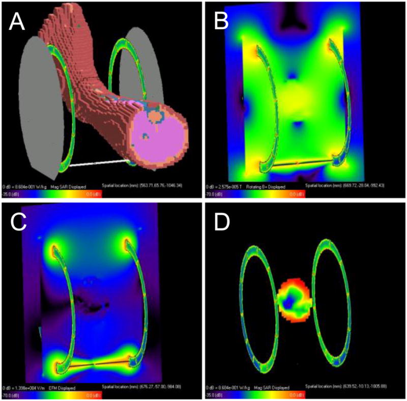
SAR simulations in a human leg: A) XFDTD mesh model, B) magnitude ${\text{B}}_1^{+}$ transmit field in an axial plane through the center of the coil and ankle, C) magnitude electric field in the same axial plane, D) SAR distribution in the same axial plane.

Fig. 3.

SAR estimation in a 50 mM saline phantom: A) XFDTD mesh model, B) magnitude ${\text{B}}_1^{+}$ transmit field in an axial plane through the center of the coil and phantom, C) SAR distribution in the same axial plane. D) Measured flip angle map (α = 30°) in a real 50 mM saline phantom of the same size (scale bar in degrees), showing a polarization pattern similar to that in (B).

Table 1.

Simulated peak/average SAR ratio at 7 T for 50 mM NaCl cylinders of different diameters

Diameter (cm)	1 g SAR Ratio	10 g SAR Ratio
2	1.3	1.1
4	2.7	1.3
6	3.4	2.2
7	3.7	2.8
8	3.3	2.6
10	2.8	2.6
12	2.5	2.3

In the heating experiment, temperature was observed to rise during the HASTE scans from a baseline of 19.1 °C to 20.1 °C (Fig. 4). Thus the total temperature rise was 1 °C. After the HASTE scans were completed, temperature fluctuated slightly from 20.1 °C to 20.2 °C. Using the specific heat capacity of water (4.18 J/g/°C), the total energy deposited in the 300 g of water in the phantom during the HASTE scans was 1254 J. Since this occurred over 64 minutes, the average rate of RF energy absorption, i.e., average SAR, in the 300-g, 6-cm diameter phantom was 1.09 W/kg. Using Table 1, this could be converted to peak SAR in 1 g or 10 g by multiplying by the appropriate factor.

Fig. 4.

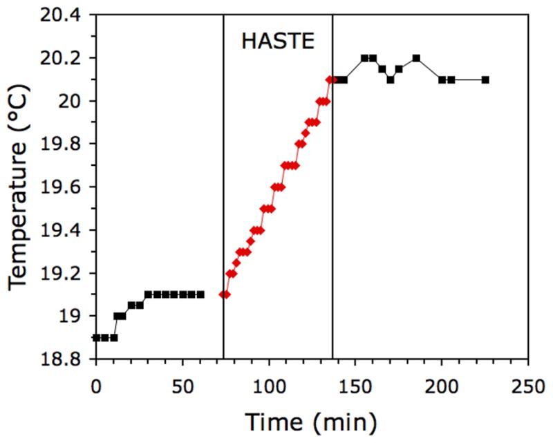
Measured temperature increase in a 50 mM saline phantom during HASTE scanning.

In order to assure safe operation of the transmit coil within the IEC and FDA SAR guidelines for non-significant risk, a K value was calculated using the above results from the phantom. The IEC values have been adopted for MRI safety in Siemens scanners, and so we used these in the following derivation. The IEC limit for peak SAR in the extremities, e.g., the distal tibia, is 20 W/kg in any 10 g of tissue, averaged over a 6-minute period. Since temperature of the phantom linearly increased during the 64 minutes of HASTE scanning, a 6-minute rate is the same as the average rate (1.09 W/kg). To convert average SAR to peak SAR that occurred in a 10 g region of the phantom we multiplied this average rate by the peak/average ratio from Table 1, i.e., (1.09 W/kg)(2.2) = 2.40 W/kg. Treating the phantom as a surrogate for the ankle, this corresponded to %SAR = (2.40/20) ×100 = 12%. Since the scanner calculated %SAR = 83% for the HASTE sequence, K could have been decreased from 0.2 kg⁻¹ to (0.2)(12/83) = 0.03 kg⁻¹ and %SAR would still have been below 100%. Hence we could have run the in vivo scans with K = 0.03 kg⁻¹. However, due to uncertainties of experimental losses in the SAR simulations, we chose to use the worst-case 1 g peak/average SAR ratio from Table 1 (3.7), together with the more restrictive FDA SAR guidelines for average SAR in the head (3 W/kg). These resulted in K = 0.32 kg⁻¹, providing more than an order of magnitude safety margin for in vivo imaging.

3.3. Transmit-receive coil performance

For the transmit coil loaded with a human ankle, S₁₁ reflection measured on a network analyzer was less than −35 dB, demonstrating good impedance match. Using the oil phantom, although the impedance match both for transmit and receive coils was not optimal, uncombined images showed the four receive elements functioning with good mutual isolation (Fig. 5), with the combined image giving an impression of the ${\text{B}}_1^{-}$ field distribution. The receive-field non-uniformity was not a significant impediment to performance, as the FSE-OSC turbo spin echo sequence produced in vivo images at 7 T in which fine trabeculae are clearly visible throughout the tibia (Fig. 6). Mean SNR at 7 T in the fatty bone marrow of the distal tibia for the three volunteers was 26 ± 4. In vivo MR images of the distal tibia of Subject #1 acquired at 1.5 T, 3 T, and 7 T using the same pulse sequence and identical parameters at each field are shown in Fig. 6 with the same relative size scale. Image data acquired at 1.5 T and at 3 T were registered to the data acquired at 7 T using sinc interpolation with both trabecular and cortical bone of the tibia as landmarks. Zoomed views of a central region in the tibia also are shown, demonstrating the clear improvement in image quality due to increased SNR, as well as the high precision of the registration.

Fig. 5.

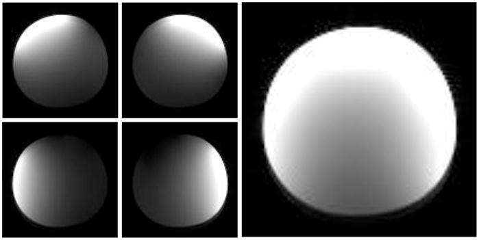
Gradient echo images of an oil phantom acquired at 7 T using the transmit-receive coil assembly, showing the four uncombined channels and the combined image.

Fig. 6.

(top row) In vivo MR images of the distal tibia of Subject #1 acquired at 1.5 T, 3 T, and 7 T, using the same pulse sequence and identical parameters. Image data acquired at 1.5 T and at 3 T were registered to the data acquired at 7 T using trabecular and cortical bone of the tibia with sinc interpolation. (bottom row) Zoomed views of a central region in the tibia.

Results of SNR measurements are listed in Table 2 and plotted in Fig. 7. In Fig. 7, average in vivo SNR versus field strength, measured at the same location in the distal tibia on registered images acquired at 1.5 T, 3 T, and 7 T for three subjects, revealed an approximately linear dependence (black squares) with a good linear fit (R² = 0.996) of the form SNR ∞ B₀ (solid line). Average SNR gain at 7 T compared to 3 T and 1.5 T was 2.8x and 4.9x, respectively. Finally, Fig. 8 shows an in vivo MR image of the distal tibia of Subject #1, acquired at 7 T with 160 μm isotropic resolution using the FSE-OSC sequence with modified parameters. The zoomed view of a central region in the tibia shows clearly visible trabeculae (SNR = 16.9).

Table 2.

In vivo SNR measured at different field strengths

	Age (years)	1.5 T	3 T	7 T
Subject #1	36	5.62	11.57	33.16
Subject #2	26	5.76	10.45	23.28
Subject #3	30	4.61	6.15	21.72
Average ± SE	31 ± 3	5.3 ± 0.4	9 ± 2	26 ± 4
Average/S8*		7.7	15	56

^*S₈ is a correction for field-dependent T₁ saturation effects (see text).

Fig. 7.

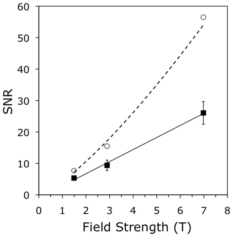
Average SNR in vivo versus field strength, measured at the same location in the distal tibia on registered images acquired at 1.5 T, 3 T, and 7 T, for three subjects. Measured values (black squares) have an approximately linear dependence, confirmed by a linear fit (R² = 0.996) of SNR ∞ B₀ (solid line). Values corrected for differential T₁ saturation (white circles) show a super-linear dependence: $\text{SNR}\propto {\text{B}}_0^{1.3}$ (dotted line).

Fig. 8.

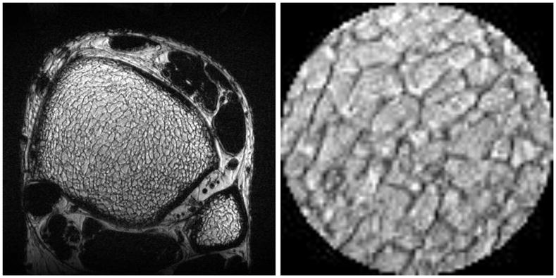
In vivo MR image of the distal tibia of Subject #1 acquired at 7 T, with 160 μm isotropic resolution. The zoomed view of a central region in the tibia shows good visibility of trabeculae (SNR = 16.9).

4. Discussion

This integrated transmit-receive coil performed very well for in vivo trabecular bone imaging at 7 T. Since the transmit coil was designed using a single human ankle for a load, the reference voltage required for a 180° flip angle varied slightly depending on the size of ankle in the coil. This has implications for sequences operating at the SAR limit, since a non-optimal load will require a higher reference voltage, possibly generating %SAR greater than 100%. Thus a modification of the parameters might be necessary for the sequence to run. This was required in the present study and achieved by reducing the flip angle of the last refocusing pulse from 90° to 50° and 60° for Subjects #2 and #3, a change that had negligible effect on SNR (17). Alternatively, using a higher acceleration could be a means to avoid the SAR limit. However, our experiments (not shown) have indicated that acceleration factors higher than 2 tend to degrade the quality of the resulting images under this imaging protocol. Reference voltages used here were 437 V, 433 V, and 407 V, and %SAR was 96%, 99%, and 95%, for Subjects #1, #2, and #3, respectively. SNR was observed to increase approximately linearly with field strength in three volunteers, consistent with nearly ideal receive coil operation as discussed below.

Method of Moments-based simulations provided a useful means to design an optimal transmit coil with a Helmholtz-pair geometry. For comparison, an additional simulation was performed for a standard birdcage coil. The choice for this was a 7-inch diameter, 8-strut, shielded low-pass birdcage coil, split into two inductively-coupled halves, and driven via a port (break) in an end-ring of the birdcage. The results gave $\mathrm{\Delta }{\text{B}}_1^{+}=14.0\%$, with C_tune/C_match = 0.8/45 pF. Even though tuning and matching could be achieved in simulations, this would be difficult to implement because each of the eight tuning capacitors would have to be tuned separately to yield a low $\mathrm{\Delta }{\text{B}}_1^{+}$. Moreover, the computed C_tune values are too small for practical implementation. While a birdcage coil with still lower $\mathrm{\Delta }{\text{B}}_1^{+}$ might be possible, its general shape is not accommodating to the foot, and it was therefore concluded that a shielded Helmholtz coil is a more practical and robust design for the present application.

Simulations also provided a means to assess the frequency-dependent performance of the four-element receive coils. From the known actual values of tuning and matching capacitors used to construct the receive coils at each field strength, loaded and unloaded Q values (Q_L and Q_U) could be estimated by the Method of Moments, from which the percent RF noise power due to the sample or load, i.e., the load loss, could be calculated as P_load = (1 − Q_L/Q_U) × 100. In an ideal receive coil, all noise would arise from the load, rather than from the coil itself, and load loss can dominate other mechanisms at higher frequencies, resulting in behavior closer to that of an ideal coil. The Q simulations showed that the receive coil elements were operating in the sample-noise dominated regime (load loss > 50%), although not to an equal degree: P_load = 66%, 80%, and 95% for the 1.5 T, 3 T, and 7 T coils, respectively. Therefore, since SNR generally increases linearly with field strength when P_load ≈ 100% and as ${\text{B}}_0^{7/4}$ for the coil-noise dominated regime (P_load ≈ 0%) (26), SNR here would be expected to increase super-linearly as ${\text{B}}_0^x$, where 1 < x < 1.75, other conditions being equal at each field. The Q simulations also suggest that P_load for the receive coils at 1.5 T and at 3 T can be increased further, possibly by increasing the size of the array elements although doing so would not necessarily increase SNR.

Without discounting the possibility of non-optimal coil performance in the form of imperfect inter-element and transmit-receive decoupling, the measured approximately linear dependence of SNR versus B₀ (Fig. 7) suggests either that the receive coils all are operating as nearly ideal coils (P_load ≈ 100%), or that other field-dependent effects on the noise and the signal could be modifying SNR. For example, noise might be modified by field-dependent g-factors and signal might be reduced due to differential spin saturation as T₁ increases at higher field. To examine these effects, first we repeated the SNR measurements on low-resolution images reconstructed without GRAPPA from the same in vivo data using only the 30 contiguous k-space calibration lines. These gave a super-linear dependence of SNR with field strength, $\text{SNR}\propto {\text{B}}_0^{1.26}$, indicating possible g-factor effects. Then we computed an upper bound on the amount of T₁ saturation in the SNR measurements using an equation previously derived (27) for the normalized steady-state signal after an excitation pulse followed by a series of 180° refocusing pulses:

$$S_n=\frac{1-{(-1)}^n{e}^{-\text{TR}/{\text{T}}_1}-2{\displaystyle \sum _{j=1}^n}{(-1)}^{n-j}{e}^{-(\text{TR}-{\tau }_j)/{\text{T}}_1}}{1-{(-1)}^{n}cos(\varphi )e^{-\text{TR}/{\text{T}}_1}}sin(\varphi )$$ (3)

An analytic expression such as this does not exist for a series of refocusing pulses of arbitrary flip angles, such as for the linear decrease in flip angle from 180° to 90° as used in this study. However, assuming all the refocusing pulses were 180°, maximal T₁ saturation effects could be calculated at each field strength, knowing the T₁ of fat and recalling that the excitation pulse = 90°, TR/TE = 500/20 ms, and the interpulse delay τ_j = 10 + 20 (n − 1) ms for n = 1…8 with eight echoes per TR. At 7 T, T₁ of fat in bone marrow is 550 ms (28). Thus S₈ (7T) = 0.4611. Furthermore, T₁ of marrow fat at 1.5 T is 288 ms and at 3 T is 365 ms (29). Hence S₈ (1.5T) = 0.6930 and S₈ (3T) = 0.6061. Therefore, the maximal correction for T₁ effects was obtained by dividing the measured SNR at each field strength by the corresponding value of S₈, the steady-state signal after eight 180° pulses (Table 2). When the SNR values were corrected for maximal differential T₁ saturation (Fig. 7, white circles), they showed a super-linear dependence given by a power-law fit of $\text{SNR}\propto {\text{B}}_0^{1.30}$ (Fig. 7, dotted line). Both of the above effects could have contributed to the measured approximately linear dependence of SNR on field strength.

In conclusion, while there are many challenges associated with imaging at 7 T, initial experience has proved to be promising for the imaging of trabecular bone at high field. It will be interesting to run full VBB processing algorithms on image data acquired at different field strengths to see how much the derived topological parameters vary with field. Such differences might arise due to imperfect refocusing of B₀-dependent static dephasing occurring near the interfaces between trabeculae and marrow, resulting in apparent thickening of trabeculae (30,31). Volume reorientation and registration with sinc interpolation, as used in the present study for SNR comparison, will be essential for these morphological measurements, but even more for the newly emerging methods of in vivo micro-mechanical testing (32,33). Moreover, the utility of high-quality 160 μm isotropic data as shown in Fig. 8, for example in capturing the fenestration of trabecular plates, has been discussed recently (34–37) and will be important for future studies.

Appendix. Circuit details for the transmit and receive coils

Circuit diagrams for the Helmholtz transmit coil and for one channel of the four-element receive coil (7 T version) are shown in Fig. A1. In the transmit coil schematics, diode D1 is for active tuning/detuning during transmit/receive and inductors L3 and L4 (1200 nH) are for filtering out RF. Capacitors C6 and C7 (10 pF) and inductor L2 (30 nH) are components of a 90° phase shifter. C4 (5.6 pF) is a matching capacitor. The drawing also has three tuning capacitors (C1, C2, C3), although in reality there are 22 tuning capacitors in series in the transmit coil (11 in each loop, 6.2 pF each) with one current path. Additional component values: C3 range = 1–10 pF, C5 = 68 pF, C8 = 820 pF, and L1 = 4.2 nH. The 90° phase shifter is used because the transmit coil has to be tuned when the PIN bias is on (positive voltage applied). For example, during transmit the PIN bias is on and diode D1 is then a short for RF. The effect of the 90° phase shifter is that the impedance changes from zero to a high value. This means that current flow through L1 is suppressed and the coil is tuned. However, during receive the PIN bias is off (negative voltage applied) and the diode is open. The phase shifter then makes this look like an RF short, so effectively L1 shorts to ground. Then capacitor C5 and inductor L1 are in parallel, and because they were selected to resonate with each other, the resulting parallel LC network has high impedance. This suppresses current flow in the Helmholtz loops and so the coil is detuned.

Fig. A1.

RF coil circuit diagrams: A) the Helmholtz-pair transmit coil; B) one channel of the 7 T four-element receive array. Note that in (A), the Helmholtz pair is drawn as a single loop consisting of capacitors C1-C5, since the two loops form a single current path and in the actual coil C1 and C2 each represent eleven capacitors spaced around each loop.

In the receive coil schematics, C1, C2, and C3 are tuning capacitors of 7.5 pF each and C4 is a matching capacitor of 22 pF. Inductor L1 was adjusted to resonate with C4. Diode D1 is for active detuning during transmit and inductors L2, L3, and L4 (1200 nH) and capacitors C6 and C7 (820 pF) are for filtering out RF. Crossed diodes D2 are for passive detuning during transmit and capacitor C5 (820 pF) is to block DC to the preamp. In addition, C3 represents two capacitors in parallel (7.5 pF and a 0.5–2.5 pF variable) so its range is 8–10 pF. The preamp gain is 25–27 dB with noise figure 0.4 dB.

References

- 1.Regatte RR, Schweitzer ME. Ultra-high-field MRI of the musculoskeletal system at 7.0T. J Magn Reson Imaging. 2007;25(2):262–9. doi: 10.1002/jmri.20814. [DOI] [PubMed] [Google Scholar]
- 2.Krug R, Carballido-Gamio J, Banerjee S, Stahl R, Carvajal L, Xu D, Vigneron D, Kelley DA, Link TM, Majumdar S. In vivo bone and cartilage MRI using fully-balanced steady-state free-precession at 7 tesla. Magn Reson Med. 2007;58(6):1294–8. doi: 10.1002/mrm.21429. [DOI] [PubMed] [Google Scholar]
- 3.Krug R, Stehling C, Kelley DAC, Majumdar S, Link TM. Imaging of the Musculoskeletal System In Vivo Using Ultra-high Field Magnetic Resonance at 7 T. Investigative Radiology. 2009;44 (9):613–618. doi: 10.1097/RLI.0b013e3181b4c055. [DOI] [PubMed] [Google Scholar]
- 4.Vaughan JT, Snyder CJ, DelaBarre LJ, Bolan PJ, Tian J, Bolinger L, Adriany G, Andersen P, Strupp J, Ugurbil K. Whole-body imaging at 7T: Preliminary results. Magnetic Resonance in Medicine. 2009;61(1):244–248. doi: 10.1002/mrm.21751. [DOI] [PMC free article] [PubMed] [Google Scholar]
- 5.Snyder CJ, DelaBarre L, Metzger GJ, Moortele P-Fvd, Akgun C, Ugurbil K, Vaughan JT. Initial results of cardiac imaging at 7 tesla. Magnetic Resonance in Medicine. 2009;61(3):517–524. doi: 10.1002/mrm.21895. [DOI] [PMC free article] [PubMed] [Google Scholar]
- 6.Guo XE, Kim CH. Mechanical consequence of trabecular bone loss and its treatment: a three-dimensional model simulation. Bone. 2002;30(2):404–11. doi: 10.1016/s8756-3282(01)00673-1. [DOI] [PubMed] [Google Scholar]
- 7.Wehrli FW. Structural and functional assessment of trabecular and cortical bone by micro magnetic resonance imaging. J Magn Reson Imaging. 2007;25(2):390–409. doi: 10.1002/jmri.20807. [DOI] [PubMed] [Google Scholar]
- 8.Wehrli FW, Song HK, Saha PK, Wright AC. Quantitative MRI for the assessment of bone structure and function. NMR Biomed. 2006;19(7):731–64. doi: 10.1002/nbm.1066. [DOI] [PubMed] [Google Scholar]
- 9.Majumdar S. Magnetic Resonance Imaging of Trabecular Bone Structure. Topics in Magnetic Resonance Imaging. 2002;13(5):323–334. doi: 10.1097/00002142-200210000-00004. [DOI] [PubMed] [Google Scholar]
- 10.Wehrli FW, Ladinsky GA, Jones C, Benito M, Magland J, Vasilic B, Popescu AM, Zemel B, Cucchiara AJ, Wright AC, Song HK, Saha PK, Peachey H, Snyder PJ. In vivo magnetic resonance detects rapid remodeling changes in the topology of the trabecular bone network after menopause and the protective effect of estradiol. J Bone Miner Res. 2008;23(5):730–40. doi: 10.1359/JBMR.080108. [DOI] [PMC free article] [PubMed] [Google Scholar]
- 11.Benito M, Vasilic B, Wehrli FW, Bunker B, Wald M, Gomberg B, Wright AC, Zemel B, Cucchiara A, Snyder PJ. Effect of testosterone replacement on trabecular architecture in hypogonadal men. J Bone Miner Res. 2005;20(10):1785–91. doi: 10.1359/JBMR.050606. [DOI] [PubMed] [Google Scholar]
- 12.Chesnut CH, Majumdar S, Newitt DC, Shields A, Pelt JV, Laschansky E, Azria M, Kriegman A, Olson M, Eriksen EF, Mindeholm L. Effects of Salmon Calcitonin on Trabecular Microarchitecture as Determined by Magnetic Resonance Imaging: Results From the QUEST Study. Journal of Bone and Mineral Research. 2005;20(9):1548–1561. doi: 10.1359/JBMR.050411. [DOI] [PMC free article] [PubMed] [Google Scholar]
- 13.Wehrli FW, Leonard MB, Saha PK, Gomberg BR. Quantitative high-resolution magnetic resonance imaging reveals structural implications of renal osteodystrophy on trabecular and cortical bone. J Magn Reson Imaging. 2004;20(1):83–9. doi: 10.1002/jmri.20085. [DOI] [PubMed] [Google Scholar]
- 14.Wright AC, Wald M, Connick T, Magland J, Song HK, Vasilic B, Lemdiasov R, Ludwig R, Wehrli FW. 7T Transmit Four-Channel Receive Array for High-Resolution MRI of Trabecular Bone in the Distal Tibia. Proceedings of ISMRM 17th Scientific Meeting; Honolulu, Hawaii. 2009. p. 2996. [Google Scholar]
- 15.Lemdiasov R, Ludwig R, Bogdanov G. Procedure for RF Coil Array Analysis Using the Method of Moments. Proceedings of ISMRM 17th Scientific Meeting; Honolulu, Hawaii. 2009. p. 1506. [Google Scholar]
- 16.Rao S, Wilton D, Glisson A. Electromagnetic scattering by surfaces of arbitrary shape. Antennas and Propagation, IEEE Transactions. 1982;30(3):409–418. [Google Scholar]
- 17.Magland JF, Rajapakse CS, Wright AC, Acciavatti R, Wehrli FW. 3D fast spin echo with out-of-slab cancellation: A technique for high-resolution structural imaging of trabecular bone at 7 tesla. Magnetic Resonance in Medicine. 2010;63(3):719–727. doi: 10.1002/mrm.22213. [DOI] [PMC free article] [PubMed] [Google Scholar]
- 18.Yang QX, Wang J, Collins CM, Smith MB, Zhang X, Ugurbil K, Chen W. Phantom design method for high-field MRI human systems. Magnetic Resonance in Medicine. 2004;52(5):1016–1020. doi: 10.1002/mrm.20245. [DOI] [PubMed] [Google Scholar]
- 19.Patel MR, Klufas RA, Alberico RA, Edelman RR. Half-fourier acquisition single-shot turbo spin-echo (HASTE) MR: comparison with fast spin-echo MR in diseases of the brain. AJNR Am J Neuroradiol. 1997;18(9):1635–40. [PMC free article] [PubMed] [Google Scholar]
- 20.Rohrer M, Bauer H, Mintorovitch J, Requardt M, Weinmann H-J. Comparison of magnetic properties of MRI contrast media solutions at different magnetic field strengths. Investigative Radiology. 2005;40(11):715–724. doi: 10.1097/01.rli.0000184756.66360.d3. [DOI] [PubMed] [Google Scholar]
- 21.Wang J, Mao W, Qiu M, Smith MB, Constable RT. Factors influencing flip angle mapping in MRI: RF pulse shape, slice-select gradients, off-resonance excitation, and B0 inhomogeneities. Magn Reson Med. 2006;56(2):463–468. doi: 10.1002/mrm.20947. [DOI] [PubMed] [Google Scholar]
- 22.Wang Z, Wang J, Detre JA. Improved data reconstruction method for GRAPPA. Magnetic Resonance in Medicine. 2005;54(3):738–742. doi: 10.1002/mrm.20601. [DOI] [PubMed] [Google Scholar]
- 23.Lin W, Ladinsky GA, Wehrli FW, Song HK. Image metric-based correction (autofocusing) of motion artifacts in high-resolution trabecular bone imaging. J Magn Reson Imaging. 2007;26(1):191–7. doi: 10.1002/jmri.20958. [DOI] [PubMed] [Google Scholar]
- 24.Magland JF, Jones CE, Leonard MB, Wehrli FW. Retrospective 3D registration of trabecular bone MR images for longitudinal studies. Journal of Magnetic Resonance Imaging. 2009;29(1):118–126. doi: 10.1002/jmri.21551. [DOI] [PMC free article] [PubMed] [Google Scholar]
- 25.Brunner DO, De Zanche N, Frohlich J, Paska J, Pruessmann KP. Travelling-wave nuclear magnetic resonance. Nature. 2009;457(7232):994–998. doi: 10.1038/nature07752. [DOI] [PubMed] [Google Scholar]
- 26.Hoult DI, Lauterbur PC. The sensitivity of the zeugmatographic experiment involving human samples. J Magn Reson. 1979;34:425–433. [Google Scholar]
- 27.Magland J, Vasilic B, Wehrli FW. Fast low-angle dual spin-echo (FLADE): a new robust pulse sequence for structural imaging of trabecular bone. Magn Reson Med. 2006;55(3):465–71. doi: 10.1002/mrm.20789. [DOI] [PubMed] [Google Scholar]
- 28.Ren J, Dimitrov I, Sherry AD, Malloy CR. Composition of adipose tissue and marrow fat in humans by 1H NMR at 7 Tesla. J Lipid Res. 2008;49(9):2055–62. doi: 10.1194/jlr.D800010-JLR200. [DOI] [PMC free article] [PubMed] [Google Scholar]
- 29.Gold GE, Han E, Stainsby J, Wright G, Brittain J, Beaulieu C. Musculoskeletal MRI at 3.0 T: Relaxation Times and Image Contrast. Am J Roentgenol. 2004;183(2):343–351. doi: 10.2214/ajr.183.2.1830343. [DOI] [PubMed] [Google Scholar]
- 30.Techawiboonwong A, Song HK, Magland JF, Saha PK, Wehrli FW. Implications of pulse sequence in structural imaging of trabecular bone. J Magn Reson Imaging. 2005;22(5):647–55. doi: 10.1002/jmri.20432. [DOI] [PubMed] [Google Scholar]
- 31.Krug R, Carballido-Gamio J, Banerjee S, Burghardt AJ, Link TM, Majumdar S. In vivo ultra-high-field magnetic resonance imaging of trabecular bone microarchitecture at 7 T. Journal of Magnetic Resonance Imaging. 2008;27(4):854–859. doi: 10.1002/jmri.21325. [DOI] [PubMed] [Google Scholar]
- 32.Rajapakse CS, Magland J, Zhang XH, Liu XS, Wehrli SL, Guo XE, Wehrli FW. Implications of noise and resolution on mechanical properties of trabecular bone estimated by image-based finite-element analysis. J Orthop Res. 2009;27(10):1263–71. doi: 10.1002/jor.20877. [DOI] [PMC free article] [PubMed] [Google Scholar]
- 33.Liu XS, Zhang XH, Rajapakse CS, Wald MJ, Magland J, Sekhon KK, Adam MF, Sajda P, Wehrli FW, Guo XE. Accuracy of high-resolution in vivo micro magnetic resonance imaging for measurements of microstructural and mechanical properties of human distal tibial bone. J Bone Miner Res. 2010;25(9):2039–2050. doi: 10.1002/jbmr.92. [DOI] [PMC free article] [PubMed] [Google Scholar]
- 34.Magland JF, Wehrli FW. Trabecular bone structure analysis in the limited spatial resolution regime of in vivo MRI. Acad Radiol. 2008;15(12):1482–93. doi: 10.1016/j.acra.2008.05.015. [DOI] [PMC free article] [PubMed] [Google Scholar]
- 35.Li CQ, Magland JF, Rajapakse CS, Guo XE, Zhang XH, Vasilic B, Wehrli FW. Implications of resolution and noise for in vivo micro-MRI of trabecular bone. Med Phys. 2008;35(12):5584–94. doi: 10.1118/1.3005598. [DOI] [PMC free article] [PubMed] [Google Scholar]
- 36.Magland JF, Wald MJ, Wehrli FW. Spin-echo micro-MRI of trabecular bone using improved 3D fast large-angle spin-echo (FLASE) Magn Reson Med. 2009;61(5):1114–21. doi: 10.1002/mrm.21905. [DOI] [PMC free article] [PubMed] [Google Scholar]
- 37.Wald MJ, Magland JF, Rajapakse CS, Wehrli FW. Structural and mechanical parameters of trabecular bone estimated from in vivo high-resolution magnetic resonance images at 3 tesla field strength. J Magn Reson Imaging. 2010;31(5):1157–68. doi: 10.1002/jmri.22158. [DOI] [PMC free article] [PubMed] [Google Scholar]