

Abstract
Motivation: With complex traits and diseases having potential genetic contributions of thousands of genetic factors, and with current genotyping arrays consisting of millions of single nucleotide polymorphisms (SNPs), powerful high-dimensional statistical techniques are needed to comprehensively model the genetic variance. Machine learning techniques have many advantages including lack of parametric assumptions, and high power and flexibility.
Results: We have applied three machine learning approaches: Random Forest Regression (RFR), Boosted Regression Tree (BRT) and Support Vector Regression (SVR) to the prediction of warfarin maintenance dose in a cohort of African Americans. We have developed a multi-step approach that selects SNPs, builds prediction models with different subsets of selected SNPs along with known associated genetic and environmental variables and tests the discovered models in a cross-validation framework. Preliminary results indicate that our modeling approach gives much higher accuracy than previous models for warfarin dose prediction. A model size of 200 SNPs (in addition to the known genetic and environmental variables) gives the best accuracy. The R2 between the predicted and actual square root of warfarin dose in this model was on average 66.4% for RFR, 57.8% for SVR and 56.9% for BRT. Thus RFR had the best accuracy, but all three techniques achieved better performance than the current published R2 of 43% in a sample of mixed ethnicity, and 27% in an African American sample. In summary, machine learning approaches for high-dimensional pharmacogenetic prediction, and for prediction of clinical continuous traits of interest, hold great promise and warrant further research.
Contact: cduarte@uab.edu
Supplementary information: Supplementary data are available at Bioinformatics online.
1 INTRODUCTION
1.1 Machine learning techniques for genomic association and predictive modeling
Machine learning techniques have been widely used in the analysis of genetic data with many examples in the field of gene expression (see for example Furey et al., 2000; Shipp et al., 2002; Hang et al., 2005) and more recently using genotypic data sources such as single nucleotide polymorphisms (SNPs) (Ban et al., 2010; Goldstein et al., 2010; Okser et al., 2010; Szymczak et al., 2009; Uhmn et al., 2009; Wei et al., 2009). In one study, the Support Vector Machine (SVM) algorithm was applied to P-value filtered genome-wide SNP data for type I diabetes (T1D), and predictive accuracy was verified in two independent cohorts in which a C-statistic of 0.84 was obtained (Wei et al., 2009). Prediction of extreme classes of atherosclerosis risk using stratification based on quantitative ultrasound imaging of carotid artery intima-media thickness (IMT) using a naïve Bayes classifier technique for both SNP selection and predictive model building was performed in Okser et al., 2010, and a C-statistic of 0.844 was obtained versus 0.761 obtained from clinical variables alone. Importantly, in both studies ( Okser et al., 2010; Wei et al., 2009) the investigators found that much greater predictive accuracy was obtained when including a large number of SNPs, and comparatively poorer performance was obtained when including only the SNPs found to have genome-wide significance. In Uhmn et al., 2009, machine learning approaches were used to discriminate chronic hepatitis in a case–control candidate SNP study, with maximum accuracy between 67% and 73% found depending on the technique used (where accuracy was defined as the total number of correctly classified samples divided by the total number of samples).
Investigators have also applied machine learning techniques to genome-wide association study (GWAS) data for gene discovery (Ban et al., 2010; Goldstein et al., 2010; Szymczak et al., 2009). Random Forests were used to find additional associated variants in four genes in a GWAS of multiple sclerosis (Goldstein et al., 2010). Prediction and gene discovery were both achieved when the authors applied machine learning techniques to type II diabetes in a Korean cohort in a candidate SNP study (Ban et al., 2010). In this study, a 65.3% prediction rate was achieved with 14 SNPs in 12 genes using the radial basis function (RBF)-kernel SVM, and additionally novel associations between certain SNP combinations and type II diabetes were obtained (in this study overall prediction rate was defined as the number of correctly classified subjects, either case or control, divided by the total number of subjects). Various machine learning techniques were tested to discover disease SNP associations in simulated and experimental GWAS datasets as part of the Genetic Analysis Workshop (Szymczak et al., 2009), and many advantages were found in using machine learning techniques over traditional statistical techniques, although it was noted that implementation of methods and variable selection techniques specific for GWAS data are needed.
Machine learning techniques have many advantages including robustness to parametric assumptions, high power and accuracy, ability to model non-linear effects, many well-developed algorithms, and the ability to model high-dimensional data. However, as previously noted (Szymczak et al., 2009), implementation of these methods in high-dimensional GWAS data is not trivial, and many details involving variable selection and algorithm parameter selection need to be optimized. Most existing studies have dealt only with candidate SNP data (for instance Ban et al., 2010; Okser et al., 2010; Uhmn et al., 2009) in which at most hundreds of SNPs are modeled. Genome-wide data are analyzed in Goldstein et al. (2010), Szymczak et al. (2009) and Wei et al. (2009), although gene-finding was the main goal in two of these (Goldstein et al., 2010; Szymczak et al., 2009).
A simplistic but effective variable selection technique of using a P-value threshold from single marker analysis is used to reduce the number of SNPs from hundreds of thousands to hundreds in (Wei et al., 2009), and we use a similar strategy here. However, in our study we model a continuous rather than a dichotomous trait, and we investigate the performance of three commonly used machine learning approaches that are specific for modeling continuous data: Random Forest Regression (RFR), Boosted Regression Tree (BRT) and Support Vector Regression (SVR).
1.2 Warfarin dose prediction
Treatment with warfarin, the most widely used oral anticoagulant agent worldwide, is complicated by the unpredictability of dose requirements and variability in anticoagulation control due to the multitude of factors that influence warfarin pharmacokinetics and pharmacodynamics. Given the narrow therapeutic index of warfarin, this variability is often associated with hemorrhagic complications. To mitigate the risk-associated response variability, investigators and clinicians have focused on developing strategies to improve dose prediction with the hopes of improving anticoagulation control with resultant decrease in hemorrhage. The recent seminal work of the IWPC demonstrates that clinical factors account for 26% of the variability in dose, which is improved to 43% by incorporation of CYP2C9 and VKORC1 genotypes (The International Warfarin Pharmacogenetics Consortium, 2009), two genes of demonstrated significance in explaining warfarin dose–response (Limdi and Veenstra, 2008). The ability of clinical and genetic factors to predict dose is significantly higher among patients of European descent (50–70%) as compared to those of African descent (25–40%) (Gage et al., 2008; Limdi et al., 2008, 2010; Schelleman et al., 2008a, 2008b; Wadelius et al., 2007, 2009).
Herein we use machine learning approaches to determine if dose prediction for African American patients can be improved by incorporating many more genotypic variables. The goal of the study was to (i) develop an overall analysis pipeline that could be used to implement and test each approach (RFR, BRT and SVR); (ii) compare and contrast the advantages and disadvantages of each approach; and (iii) choose the best method and develop a new model for predicting warfarin maintenance dose in African Americans.
2 METHODS
2.1 Warfarin patient cohort, genotyping and single marker analysis
The details of the patient cohort, genetic and clinical variables collected, and initial processing of genetic data are contained in the SupplementaryMaterial. The clinical variables included age, height, weight, congestive heart failure, concurrent amiodarone use, moderate or severe chronic kidney disease (CKD) as assessed by estimated glomerular filtration rate levels and/or treatment with maintenance dialysis.
We performed whole-genome genotyping for 300 individuals using the Illumina 1M array with an overall 99.5% genotyping call rate and no gender discrepancies (six samples with call rates of <99.5% were excluded from analysis). We filtered SNPs based on a minor allele frequency of <2% due to the small sample size, and failure of the Hardy–Weinberg Equilibrium (HWE) test as assessed by a P-value of <0.001 (Purcell et al., 2007). We also removed two pairs of individuals (four individuals) with higher than expected genetic relatedness as measured in PLINK and EIGENSTRAT (Price et al., 2006), resulting in 290 as the sample size for subsequent analysis.
Single marker linear regression was performed in PLINK using the square root of warfarin dose as the response variable and including the covariates age, weight, height, congestive heart failure, moderate or severe CKD, and concurrent use of amiodarone and the first two principle components from Eigenstrat (Price et al., 2006) to control for population stratification. To identify novel markers that could improve dose prediction, we also included the following genetic variables as covariates including genetic variants within VKORC1 (rs9934438), ApoE (rs429358 and rs7412), CYP4F2 (rs2774030) and CYP2C9 (haplotype of rs1799853, *2, and rs1057910, *3).
2.2 Model building
Our entire process was contained within a five-fold cross-validation (CV) structure, with all model building steps (including SNP selection) performed in each training partition and the model evaluation performed in the respective test partition for each fold. In order to build a predictive genetic model with only the most important genetic variants, we performed a selection of SNPs at a certain P-value cutoff using linear regression in PLINK, an approach similar to that taken in Wei et al. (2009). We used the top set of SNPs (according to P-value) in set sizes between 20 and 500. We chose to use set size (number of markers), rather than P-value threshold as in Wei et al. (2009), in order to keep model sizes constant across folds. Once a set of SNPs was selected, imputation of missing values was performed using fastPHASE (Scheet and Stevens, 2006). An additive coding was used for the SNPs selected (either 0, 1 or 2 copies of the minor allele). Then the most accurate model for a given set of variables was discovered in the training partition using RFR, SVR or BRT, where model accuracy for the continuous dose–response trait is assessed using R2, the squared correlation between predicted and actual trait value (square root of warfarin dose). R2 is the measure that we will use to measure predictive accuracy of the model throughout this article. Finally, the predictive accuracy of the model was assessed in the test partition using R2 between actual and predicted trait value. The overall process is illustrated in Figure 1.
Fig. 1.
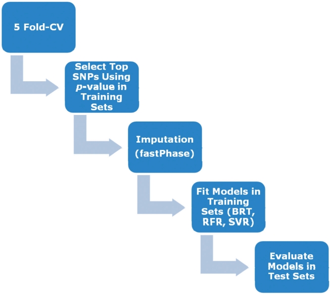
Diagram of model building pipeline including (i) subdivision of sample into testing and training partitions; (ii) SNP selection using training partition; (iii) imputation of selected SNPs using FastPhase; (iv) model building using BRT, RFR or SVR; and (v) model evaluation in testing partition.
BRT, SVR and RFR were implemented using R. We used the gbm package for BRT, the randomForest package for RFR, the ModelMap package for data manipulation and the e1071 package for SVR. Here we will briefly give some background on each approach and discuss the selection of algorithm parameters.
2.2.1 BRT
BRT makes use of Classification and Regression Tree (CART) models and boosting, and is a stagewise technique in the sense that every new tree is chosen to fit the previous tree's residuals. At the final stage BRT develops a regression model f(x) as a function of the M selected trees,
where m = 1, 2,… , M indexes the tree, βm are basis expansion coefficients, x represents the set of SNPs and b(x; γm) are the basis functions of x having parameters γm. The key algorithm parameters are the learning rate (lr) which shrinks the contribution of each tree as it is added to the model, and the number of trees (nt). In general a smaller lr and a larger nt is desirable (Elith et al., 2008), contingent on the sample size and the computational complexity. The usual approach is to estimate the optimal lr and nt (Breiman, 2001) with an independent test set or with CV, using deviance reduction as the measure of success. In our study, we estimated these parameters according to CV (within the training partition in the overall pipeline). In addition, we performed stochastic gradient boosting to fit boosted regression models, which improves predictive performance through reducing the variance of the final model by using only a random subset of data to fit each new tree (Breiman, 2001).
2.2.2 SVR
SVR (Vapnik, 1998) uses linear models to implement non-linear regression by mapping the input space to a higher dimensional feature space using kernel functions. A feature of SVR is that it simultaneously minimizes an objective function which includes both model complexity and the error in the training data (Moser et al., 2009). In ε-SV regression (Cortes and Vapnik, 1995), the goal is to find a function that has at most ε deviation from yi, and at the same time is as flat as possible (small w as defined below) (Basak et al., 2007). We can write this problem as a convex optimization problem (Moser et al., 2009; Smola and Schölkopf, 2004),
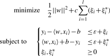 |
where w are the regression coefficients onto the kernel basis functions, C is a regularization parameter, l is the sample size, ξi and ξi* are slack variables, yi is the trait for individual i, xi is the set of SNPs for individual i, b represents the deviation from the true data value yi and ε is the tolerance margin. In our implementation, we used a Gaussian kernel which replaces the dot product listed in the primal form above,
The values of the parameters C and γ were calibrated via five-fold internal CV within the training set using the tune.svm function in the e1071 package in R (with the remaining parameter ε constrained after optimization of the other two). Such selection of C and γ from the training data (and estimated noise level) is shown to have good generalization properties for SVR over a variety of different types of datasets (Cherkassky and Ma, 2004). The parameter values estimated are shown in Supplementary Table S1.
2.2.3 RFR
RFR is an effective non-parametric statistical technique for high-dimensional analysis. Random Forests are a combination of tree predictors such that each tree depends on the values of a random vector sampled independently and with the same distribution for all trees in the forest. The tree methods exhaustively break down cases into a branched, tree-like form until the splitting of the data is statistically meaningful, with unnecessary branches pruned using other test cases to avoid overfitting (Choi and Lee, 2003). The generalization error for forests converges to a limit as the number of trees in the forest becomes large, and depends on the strength of the individual trees in the forest and the correlation between them (Breiman, 2001). Each tree in the forest is grown to the largest extent possible without pruning. To classify a new object, each tree in the forest gives a classification, which is interpreted as the tree ‘voting’ for that class. The final classification of the object is determined by majority votes among the classes decided by the forest of trees (Chen and Liu, 2005). Our algorithm additionally uses a bootstrap-based CV approach to improve performance and prevent overfitting (Cabrera, 2009). The one tuning parameter for RFR is mtry which is the number of descriptors randomly sampled for potential splitting at each node during tree induction. This parameter can range from 1 to p (the number of predictors). We used p/3 as recommended for regression (Svetnik et al., 2003), although it was noted in that article that the performance of random forest (RF) changed little over a wide range of values of mtry except near the extremes of 1 or p. The actual values of mtry used are shown in Supplementary Table S2.
3 RESULTS
We tested each machine learning technique (RFR, BRT and SVR) on a variety of different pharmacogenetic models listed in Table 1. Model 1 is similar to the previously tested model (IWPC, 2009) found to have an R2 of 43% in an independent multi-ethnic cohort. Model 2 includes the variables in Model 1 as well as some additional previously identified associated genetic variants. The remaining models include the variables from Model 2 augmented by SNPs selected using single marker analysis in PLINK (see Section 2).
Table 1.
Prediction models for square root of warfarin dose–response tested in our study
| Model | Variables |
|---|---|
| M1a | Clinical variables + VCORC1 + CYP2C9 |
| M2b | Model 1 + ApoE + CYP4F2 |
| M2 + 20 | Model 2 + best 20 SNPs |
| M2 + 50 | Model 2 + best 50 SNPs |
| M2 + 100 | Model 2 + best 100 SNPs |
| M2 + 150 | Model 2 + best 150 SNPs |
| M2 + 200 | Model 2 + best 200 SNPs |
| M2 + 300 | Model 2 + best 300 SNPs |
| M2 + 400 | Model 2 + best 400 SNPs |
| M2 + 500 | Model 2 + best 500 SNPs |
aClinical variables include age, weight, height, congestive heart failure, moderate or severe CKD, concurrent use of amiodarone and the first two principle components from Eigenstrat; VKORC1 is represented by rs9934438, and CYP2C9 is a haplotype of rs1799853 (*2) and rs1057910 (*3).
bApoE is a haplotype of rs429358 and rs7412, and CYP4F2 is rs2774030.
The R2 of each discovered model averaged over the training and testing partitions in the five-fold CV for RFR, BRT and SVR are shown in Table 2. In addition, Figure 2 shows a plot of the average R2 for each model and each technique in the test partitions.
Table 2.
Mean R2 for prediction of square root warfarin maintenance dose as measured in training and testing partitions using five-fold CV with: RFR, BRT and SVR
| Model | RFR |
BRT |
SVM |
|||
|---|---|---|---|---|---|---|
| Training | Test | Training | Test | Training | Test | |
| M1 | 25.6 (1.6) | 21.7 (1.7) | 29.5 (7.0) | 19.9 (1.5) | 24.6 (2.0) | 25.0 (2.4) |
| M2 | 30.5 (1.2) | 27.8 (2.1) | 22.5 (1.5) | 22.0 (1.6) | 30.9 (2.1) | 30.4 (1.1) |
| M2 + 20 | 35.6 (2.5) | 35.8 (1.4) | 28.1 (2.6) | 22.9 (1.5) | 32.9 (1.4) | 33.5 (2.0) |
| M2 + 50 | 44.8 (2.1) | 41.8 (1.5) | 35.1 (2.4) | 31.0 (2.4) | 36.3 (1.9) | 37.2 (2.4) |
| M2 + 100 | 50.9 (2.5) | 51.2 (2.6) | 39.4 (3.0) | 34.8 (1.5) | 44.6 (3.1) | 49.3 (2.1) |
| M2 + 150 | 58.5 (1.5) | 60.5 (1.7) | 44.4 (3.3) | 45.5 (1.4) | 54.5 (1.0) | 55.5 (2.6) |
| M2 + 200 | 66.8 (0.9) | 66.4 (1.1) | 56.2 (0.8) | 56.9 (0.7) | 58.6 (1.6) | 57.8 (1.4) |
| M2 + 300 | 58.2 (2.9) | 57.1 (1.1) | 54.6 (2.8) | 47.9 (1.3) | 56.2 (1.1) | 54.0 (1.8) |
| M2 + 400 | 55.1 (2.7) | 49.1 (1.9) | 54.1 (3.1) | 52.8 (1.8) | 54.5 (1.2) | 52.3 (3.8) |
| M2 + 500 | 53.5 (1.7) | 48.0 (1.3) | 51.5 (2.4) | 49.2 (1.4) | 53.6 (1.5) | 47.2 (4.0) |
Standard error of the mean R2 is shown in parentheses. The models are described in Table 1.
Fig. 2.

Mean and standard error of R2 in test partitions for RFR, BTR and SVR techniques averaged over five-fold CV results for different models fitted (Table 1). Standard error is given as the SD over test partitions divided by the square root of the number of test partitions.
Figure 2 shows that predictive accuracy as measured in the test partitions increases with larger models for all three methods tested until a peak at the M2+200 model, beyond which further increases in model size cause a slight decrease in predictive accuracy. One interpretation of this result is that the increased noise associated with estimating a larger and more complex model outweighs the benefit of additional variables beyond 200 SNPs, or alternatively, that Model 2 augmented by the first 200 SNPs may capture all or most of the relevant genetic (and environmental) predictors. Future testing with a larger sample size may help decide between these two hypotheses.
In terms of the overall predictive accuracy achieved as measured in the test partitions, the R2 for Model 1, which is analogous to the previously tested model (IWPC, 2009), ranges from 25% to 30%, which is less than the previously cited R2 for this model in a multi-ethnic cohort, (43%; IWPC, 2009), but is in agreement with previous estimates in populations of African descent (Gage et al., 2008; Limdi et al., 2008, 2010; Schelleman et al., 2007, 2008a, 2008b). Model 2, which contains other known associated variants for warfarin dose–response, is seen to have a modest increase in accuracy over Model 1, but significant increases in accuracy are seen with the addition of SNPs using each of the machine learning regression techniques tested. The highest predictive power was seen with RFR in which an average R2 of 66.4% was achieved with Model 2 + 200 SNPs. The other two methods tested, BRT and SVR, also show the highest predictive accuracy with the M2+200 model (56.9% for BRT and 57.8% for SVR). These R2 values are much higher than the 27% reported by the IWPC (Limdi et al., 2010) for African Americans.
Robustness of the proposed models is demonstrated in part by comparing the change in R2 from training to testing partitions (Table 2). The decrease in R2 is seen to be very small or not existent, and in general within the error of the method, which suggests that our methodology is able to guard against overfitting. In addition, the fact that the predictive accuracy of our methods show a peak at a certain model size (Model 2 + 200 SNPs) and does not continue to increase demonstrates that mechanisms for preventing overfitting in each of the three methods tested are having the desired effect.
Further improvements in predictive accuracy may be achieved if larger testing and training sets are used. Similarly, this approach may improve dose prediction for ethnic groups other than African American. Although RFR achieved the best performance in this study, all three techniques show improved prediction over the current model.
4 DISCUSSION
In this article, we have demonstrated a practical approach for applying three commonly used machine learning techniques for continuous data, RFR, SVR and BRT, to create highly accurate predictive models using genome-wide genotype data and clinical variables. In an application to prediction of warfarin dose–response in African Americans, all three methods tested, RFR, SVR and BRT, achieved better performance than currently published reports (IWPC, 2009; Limdi et al., 2010), although the highest accuracy was achieved with RFR. This may be due to the robustness of RFR to overfitting in performing bootstrapping over thousands of trees. The results of this study indicate that even with a phenotype like warfarin maintenance dose that has many validated associated genetic variants of large effect, it is still important to include a large number of genotypic variables in a predictive model to capture the most genetic variance. Our results are consistent with the findings in (Okser et al., 2010; Wei et al., 2009) that show that including only those SNPs found to have genome-wide significance in GWAS studies results in poorer predictive performance, and that much better performance is obtained with larger models.
In considering which machine learning method to apply to GWAS-based predictive modeling of a continous trait, there are many considerations. While in the present study the best performance was obtained with RFR, evaluation of these three (RFR, SVR and BRT) and other methods needs to be performed in many different studies before final conclusions can be drawn about the superiority of a particular approach. Also, it should be noted that the present study is performed in a single ethnicity (African American), and testing in sample populations of different ethnicity needs to be performed before drawing general conclusions. In general, the advantages of RFR include that variable selection is done internally and thus is not a prerequisite, it has a reliable procedure for monitoring internal predictive performance, and discovered models obtained are tolerant to noise in source experimental data. The most important disadvantage is that RFR can be potentially unreliable for variable selection when diverse variable types are included (Strobl et al., 2007), although the predictive accuracy is not expected to suffer. The main advantage of SVR is that it fits a continuous-valued function to data in a way that shares many of the advantages of SVMs classification. A disadvantage of SVR is that most algorithms (Chang and Lin, 2002; Smola and Schölkopf, 1998; Smola et al., 1998) require that the training samples be delivered in a single batch (Basak et al., 2007). As SVR is a relatively new method, more investigation is required to clarify its advantages and disadvantages, of which our study is one example. The advantages of BRT include that it can accommodate continuous and factor predictors, it automatically fits interactions, it is insensitive to monotone transforms of predictors, it allows for missing values in predictors and it ignores extraneous predictors. The disadvantages are that it can be prone to misclassification error, and it can be difficult to interpret for larger trees, although results of BRT are usually more reliable than other tree-based methods. Overall, our study confirms the conclusions of previous studies that indicate machine learning methods are suitable for high-dimensional genomic data modeling (Ban et al., 2010; Goldstein et al., 2010; Okser et al., 2010; Szymczak et al., 2009; Uhmn et al., 2009; Wei et al., 2009).
There are many areas for improvement and optimization in our approach, the most important of which may be the pre-selection of SNPs. Using a P-value threshold is convenient and fast, but may entail addition of redundant, linked predictors to the model and may not result in selection of the most complementary SNP set, although it should be noted that the machine learning techniques used can appropriately handle correlated predictors. A machine learning based variable selection step such as that used in Okser et al. (2010) may be a good alternative if it can be generalized to genome-wide data. It should also be noted that we used a constant model size (number of SNPs) rather than a set P-value threshold in exploring different-sized predictive models (Table 1) in order to keep model sizes constant across folds, otherwise it would be preferable to use preset increments in P-value threshold.
Other open research questions include the tuning and optimization of algorithm parameters for GWAS SNP data, trying new machine learning techniques such as Random Jungle (Schwarz et al., 2010) or incorporating dimension reduction prior to variable selection. Incorporation of more clinical and environmental variables as well as allowing for gene by environment interaction may also improve predictive performance. In addition, we did not explore different normalizations of the non-genetic model variables in order to keep our predictive models consistent with previously described warfarin dose–response models, and instead focused on how to best complement existing models with varying numbers of genetic predictors. However, it is possible that alternative normalizations of these parameters may give improved prediction, and this will be explored in future work. In addition, an in-depth evaluation of different machine learning methods in terms of predictive performance, robustness and computational performance in a simulation study would be valuable, as well as a comparison of machine learning versus traditional statistical approaches for prediction using genome-wide data.
Validation of the discovered models in an independent dataset is currently in progress, although use of this model in clinical practice will require model discovery in a much larger and more representative sample for fine-tuning of model parameters. However, the strong positive results from this initial study show that machine learning techniques for high-dimensional pharmacogenetic models hold much promise for improving clinical predictions of dose–response and other relevant continuous-valued clinical traits.
Supplementary Material
ACKNOWLEDGEMENTS
We would like to acknowledge the helpful discussions with David Allison, Murat Tanik, Xiang-Yang Lou, Guo-Bo Chen and Nicholas Pajewski, as well as Ergun Karaagaoglu and Erdem Karabulut who have advised E.C.
Funding: National Heart Lung and Blood Institute (RO1HL092173, in part); National Institute of Neurological Disorders and Stroke (K23NS45598).
Conflict of Interest: none declared.
REFERENCES
- Ban H., et al. Identification of type 2 diabetes associated combination of SNPs using support vector machine. BMC Genet. 2010;11:26–36. doi: 10.1186/1471-2156-11-26. [DOI] [PMC free article] [PubMed] [Google Scholar]
- Basak D., et al. Support vector regression. Neural Inform. Process. Lett. Rev. 2007;11:203–224. [Google Scholar]
- Breiman L. Random forests. Mach. Learn. 2001;45:5–32. [Google Scholar]
- Cabrera J. Course Notes of ‘Exploring/Data Mining Pharmaceutical Data’ by Birol Emir (PFIZER) - Prof., 10 MAY 2009, Pre-conference Course of IBS-EMR 2009. Istanbul, Turkey: 2009. [Google Scholar]
- Chang C.C., Lin C.J. Training ν -support vector regression: theory and algorithms. Neural Comput. 2002;14:1959–1977. doi: 10.1162/089976602760128081. [DOI] [PubMed] [Google Scholar]
- Chen X.-W., Liu M. Prediction of protein–protein interactions using random decision forest framework. Bioinformatics. 2005;21:4394–4400. doi: 10.1093/bioinformatics/bti721. [DOI] [PubMed] [Google Scholar]
- Cherkassky V., Ma Y. Practical selection of SVM parameters and noise estimation for SVM regression. Neural Netw. 2004;17:113–126. doi: 10.1016/S0893-6080(03)00169-2. [DOI] [PubMed] [Google Scholar]
- Choi E., Lee C.H. Feature extraction based on the Bhattacharyya distance. PR. 2003;36:1703–1709. [Google Scholar]
- Cortes C., Vapnik V. Support vector networks. Mach. Learn. 1995;20:273–297. [Google Scholar]
- Elith J., et al. A working guide to boosted regression trees. J. Animal Ecol. 2008;77:802–813. doi: 10.1111/j.1365-2656.2008.01390.x. [DOI] [PubMed] [Google Scholar]
- Furey T., et al. Support vector machine classification and validation of cancer tissue samples using microarray expression data. Bioinformatics. 2000;16:906–914. doi: 10.1093/bioinformatics/16.10.906. [DOI] [PubMed] [Google Scholar]
- Gage B.F., et al. Use of pharmacogenetic and clinical factors to predict the therapeutic dose of warfarin. Clin. Pharmacol. Ther. 2008;84:326–331. doi: 10.1038/clpt.2008.10. [DOI] [PMC free article] [PubMed] [Google Scholar]
- Goldstein B.A., et al. An application of Random Forests to a genome-wide association dataset: methodological considerations & new findings. BMC Genet. 2010;11:49–61. doi: 10.1186/1471-2156-11-49. [DOI] [PMC free article] [PubMed] [Google Scholar]
- Limdi N.A., Veenstra D.L. Warfarin pharmacogenetics. Pharmacotherapy. 2008;28:1084–1097. doi: 10.1592/phco.28.9.1084. [DOI] [PMC free article] [PubMed] [Google Scholar]
- Limdi N.A., et al. VKORC1 polymorphisms, haplotypes and haplotype groups on warfarin dose among African-Americans and European-Americans. Pharmacogenomics. 2008;9:1445–1458. doi: 10.2217/14622416.9.10.1445. [DOI] [PMC free article] [PubMed] [Google Scholar]
- Limdi N.A., et al. Warfarin pharmacogenetics: a single VKORC1 polymorphism is predictive of dose across three racial groups. Blood. 2010;115:3827–3834. doi: 10.1182/blood-2009-12-255992. [DOI] [PMC free article] [PubMed] [Google Scholar]
- Miners J.O., Birkett D.J. Cytochrome P4502C9: an enzyme of major importance in human drug metabolism. Br. J. Clin. Pharmacol. 2008;45:525–538. doi: 10.1046/j.1365-2125.1998.00721.x. [DOI] [PMC free article] [PubMed] [Google Scholar]
- Momary K.M., et al. Factors influencing warfarin dose requirements in African-Americans. Pharmacogenomics. 2007;8:1535–1544. doi: 10.2217/14622416.8.11.1535. [DOI] [PubMed] [Google Scholar]
- Moser G., et al. A comparison of five methods to predict genomic breeding values of dairy bulls from genome-wide SNP markers. Genet. Sel. Evol. 2009;41:56–71. doi: 10.1186/1297-9686-41-56. [DOI] [PMC free article] [PubMed] [Google Scholar]
- Okser S., et al. Genetic variants and their interactions in the prediction of increased pre-clinical carotid atherosclerosis: the cardiovascular risk in young Finns study. PLoS Genet. 2010;6:e1001146–e100158. doi: 10.1371/journal.pgen.1001146. [DOI] [PMC free article] [PubMed] [Google Scholar]
- Price A.L., et al. Principal components analysis corrects for stratification in genome-wide association studies. Nat. Genet. 2006;38:904–909. doi: 10.1038/ng1847. [DOI] [PubMed] [Google Scholar]
- Purcell S., et al. PLINK: a tool set for whole-genome association and population-based linkage analyses. Am. J. Hum. Genet. 2007;81:559–575. doi: 10.1086/519795. [DOI] [PMC free article] [PubMed] [Google Scholar]
- Rettie A.E., Jones J.P. Clinical and toxicological relevance of CYP2C9: drug-drug interactions and pharmacogenetics. Annu. Rev. Pharmacol. Toxicol. 2005;45:477–494. doi: 10.1146/annurev.pharmtox.45.120403.095821. [DOI] [PubMed] [Google Scholar]
- Schelleman H., et al. Warfarin response and vitamin K epoxide reductase complex 1 in African Americans and Caucasians. Clin. Pharmacol. Ther. 2007;81:742–747. doi: 10.1038/sj.clpt.6100144. [DOI] [PubMed] [Google Scholar]
- Schelleman H., et al. Dosing algorithms to predict warfarin maintenance dose in Caucasians and African Americans. Clin. Pharmacol. Ther. 2008a;84:332–339. doi: 10.1038/clpt.2008.101. [DOI] [PMC free article] [PubMed] [Google Scholar]
- Schelleman H., et al. Ethnic differences in warfarin maintenance dose requirement and its relationship with genetics. Pharmacogenomics. 2008b;9:1331–1346. doi: 10.2217/14622416.9.9.1331. [DOI] [PubMed] [Google Scholar]
- Schwarz D.F., et al. On safari to Random Jungle: a fast implementation of Random Forests for high-dimensional data. Bioinformatics. 2010;26:1752–1758. doi: 10.1093/bioinformatics/btq257. [DOI] [PMC free article] [PubMed] [Google Scholar]
- Shipp M., et al. Diffuse large B-cell lymphoma outcome prediction by gene-expression profiling and supervised machine learning. Nat. Med. 2002;8:68–74. doi: 10.1038/nm0102-68. [DOI] [PubMed] [Google Scholar]
- Smola A.J., Schölkopf B. On a kernel-based method for pattern recognition, regression,approximation, and operator inversion. Algorithmica. 1998;22:211–231. [Google Scholar]
- Smola A.J., Schölkopf B. A tutorial on support vector regression. Stat. Comput. 2004;14:199–222. [Google Scholar]
- Smola A., et al. General cost functions for support vector regression. In: Downs T., et al., editors. Proceedings of the Ninth Australian Conference on Neural Networks. Brisbane, Australia: University of Queensland; 1998. pp. 79–83. [Google Scholar]
- Strobl C., et al. Bias in random forest variable importance measures: illustrations, sources and a solution. BMC Bioinformatics. 2007;8:25–45. doi: 10.1186/1471-2105-8-25. [DOI] [PMC free article] [PubMed] [Google Scholar]
- Svetnik V., et al. Random forest: a classification and regression tool for compound classification and QSAR modeling. J. Chem. Inform. Comput. Sci. 2003;43:1947–1958. doi: 10.1021/ci034160g. [DOI] [PubMed] [Google Scholar]
- Szymczak S., et al. Machine learning in genome-wide association studies. Genet. Epidemiol. 2009;33(Suppl. 1):S51–S57. doi: 10.1002/gepi.20473. [DOI] [PubMed] [Google Scholar]
- The International Warfarin Pharmacogenetics Consortium. Estimation of the warfarin dose with clinical and pharmacogenetic data. New Engl. J. Med. 2009;360:753–764. doi: 10.1056/NEJMoa0809329. [DOI] [PMC free article] [PubMed] [Google Scholar]
- Uhmn S., et al. A study on application of single nucleotide polymorphism and machine learning techniques to diagnosis of chronic hepatitis. Expert Syst. 2009;26:60–69. [Google Scholar]
- Vapnik V.N. Statistical Learning Theory. New York: John Wiley & Sons; 1998. [Google Scholar]
- Wadelius M., et al. Association of warfarin dose with genes involved in its action and metabolism. Hum. Genet. 2007;121:23–34. doi: 10.1007/s00439-006-0260-8. [DOI] [PMC free article] [PubMed] [Google Scholar]
- Wadelius M., et al. The largest prospective warfarin-treated cohort supports genetic forecasting. Blood. 2009;113:784–792. doi: 10.1182/blood-2008-04-149070. [DOI] [PMC free article] [PubMed] [Google Scholar]
- Wei Z., et al. From disease association to risk assessment: an optimistic view from genome-wide association studies on type I diabetes. PLoS Genet. 2009;5:e1000678–e1000688. doi: 10.1371/journal.pgen.1000678. [DOI] [PMC free article] [PubMed] [Google Scholar]
- Yang Y., et al. Gene selection from microarray data for cancer classification—a machine learning approach. Comput. Biol. Chem. 2005;29:37–46. doi: 10.1016/j.compbiolchem.2004.11.001. [DOI] [PubMed] [Google Scholar]
Associated Data
This section collects any data citations, data availability statements, or supplementary materials included in this article.