

Abstract
A new implicit solvation model was developed for calculating free energies of transfer of molecules from water to any solvent with defined bulk properties. The transfer energy was calculated as a sum of the first solvation shell energy and the long-range electrostatic contribution. The first term was proportional to solvent accessible surface area and solvation parameters (σi) for different atom types. The electrostatic term was computed as a product of group dipole moments and dipolar solvation parameter (η) for neutral molecules, or using a modified Born equation for ions. The regression coefficients in linear dependencies of solvation parameters σi and η on dielectric constant, solvatochromic polarizability parameter π*, and hydrogen-bonding donor and acceptor capacities of solvents were optimized using 1269 experimental transfer energies from 19 organic solvents to water. The root-mean-square errors for neutral compounds and ions were 0.82 and 1.61 kcal/mol, respectively. Quantification of energy components demonstrates the dominant roles of hydrophobic effect for non-polar atoms and of hydrogen-bonding for polar atoms. The estimated first solvation shell energy outweighs the long-range electrostatics for most compounds including ions. The simplicity and computational efficiency of the model allows its application for modeling of macromolecules in anisotropic environments, such as biological membranes.
Keywords: transfer energy, accessible surface area, dipolar energy, solvent polarity, hydrogen bonding, partition coefficient
INTRODUCTION
Development of reliable, accurate and efficient methods for modeling of biologically active compounds, peptides and proteins in phospholipid membranes is an important problem in computational chemistry1–3. During the association with membranes some parts of a large molecule may remain in water, while other parts enter into the milieu of different polarity, such as the water-rich interfacial lipid head group region or the hydrophobic acyl chain region. To model this process, the highly anisotropic environment of the lipid bilayer can be approximated by one or several slabs with different dielectric properties2, 4. In a more realistic approach, the lipid bilayer may be described by continuous polarity profiles that can be obtained experimentally using different spectroscopic probes4–9 or theoretically.
In order to reproduce the behavior and energetics of complex biological systems, it is important to have a solvation model that satisfies at least three basic requirements. It should be universal to allow calculating transfer energy from water or vapor to any liquid phase10–12. It should be physics-based to describe all essential components of free energy, including hydrophobic interactions, solute-solvent hydrogen bonds and long-range electrostatics. Finally, it should be computationally efficient to be applicable for macromolecular complexes and high-throughput screening. Though a great variety of methods have been developed for the theoretical assessment of solute-solvent interactions13–15, none of them fully satisfy these requirements.
Full-atomic molecular dynamics (MD) simulations with explicit solvent provide the highest level of structural details, but at the expense of computational efficiency. Despite the algorithmic advances and significant progress in technology which allow running the MD simulations on nanosecond or even millisecond time scales16, an ab initio folding and insertion of macromolecules into biomembranes still remains a significant challenge for this approach. This led to the use of coarse-grained (GC) simulations of membrane-protein complexes, which strongly simplify molecular structure of proteins and lipids17. However, neither CG nor even more rigorous all-atom MD simulations are sufficiently accurate in predicting the free energy of solvation, because the underlying force fields neglect solvent and solute polarization18, 19 and the environment-dependence of van der Waals (vdW) forces20. Furthermore, these methods operate with the potential energy of molecules21. The calculation of free energy requires an extensive conformational sampling and estimation of the entropy of the solute-solvent system22. Small errors in the underlying force fields may accumulate during the calculations of large potential energies. Therefore, the estimations of transfer free energies by these methods are less reliable than those performed by advanced empirical continuum models 4, 23, 24.
On the other hand, solvation models based on empirical parameterization, such as Quantitative Structure Activity Relationship (QSAR) and Linear Solvation Energy Relationship (LSER) models, represent a more straightforward approach to quantitative evaluation of the solvation energy, because all parameters of these models are derived from the experimental partition coefficients that are directly related to the transfer free energy25. In these models the solute is usually considered at all-atom level or using various molecular and fragmental descriptors26, while solvent is treated implicitly as an isotropic liquid phase. However, these models are usually employed for small molecules that are fully exposed to the solvent, but not to macromolecules that have a significant fraction of solvent-inaccessible atoms.
A similar approach can be applied to larger molecules with a significant portion of buried atoms by assuming that energy of the solute-solvent interactions is proportional to the solvent-accessible surface areas (ASA) for different atom types of the macromolecular solute. The corresponding ASA are multiplied by atomic solvation parameters, σi, which are defined as solvation free energy changes per surface unit area27 A number of ASA-based implicit solvation models have been developed and successfully applied for simulation of peptides and proteins in the lipid bilayers3, 28–31. The computational efficiency of such an approach allowed us to use it for large-scale calculations of the spatial arrangement in membranes of integral proteins from the entire Protein Data Bank 3, 32, 33. However, the accuracy of these models is limited because they use a simplified “hydrophobic slab” representation of the lipid bilayer, lack the adequate representation of the complex bilayer interfaces, and do not properly define the electrostatic energy, which is included as a part of the ASA-term rather than a function of atomic charges or dipoles.
More advanced continuum solvation models have been developed to account for energy of electrostatic interactions, using, for example, the finite difference solution of the Poisson equation34 or Generalized Born method35. Some of these models were modified to deal with the heterogeneous dielectric environment of membranes by including a position-dependent scaling factor1, 36, 37. These models assume that the solvent polarity can be characterized solely by static dielectric constant (e). However, it has been well recognized that solvent strength depends on many other factors38. In particular, the importance of solute-solvent H-bonds led to development of empirical hydrogen-bonding acidity (α) and basicity (β) parameters39–42 that were proven to be important for quantification of solubility data. Moreover, the electrostatic interactions of dipoles with media can be described by the solvent solvatochromic polarity/polarizability parameter (π*) better than by macroscopic dielectric constant43, 44. While focusing on the bulk-dielectric treatment of the solvent, the continuum electrostatic models do not accurately quantify hydrogen-bonding and other interactions in the first solvation shell14, 45. Instead, the adjustment of effective atomic radii is frequently used as a simplified approach to deal with this issue 24, 35.
These problems can be resolved by combining the continuum electrostatic models with ASA-based methods that allow incorporation of the first solvation shell effects, as in a series of SMx implicit solvation models23, 46. SMx models represent the universal approach to solvation modeling, which permits prediction of transfer energies between any gaseous and condensed fluid phases23. However, due to the quantum mechanical calculations, this approach is mostly useful for small molecules in isotropic phases rather than for proteins in anisotropic environments.
Here we present a new implicit solvation model for calculating transfer energy of molecules from water to a fluid medium with defined polarity parameters. The proposed model is empirically parameterized to account for both long-range and short-range contributions to the transfer free energy. The model is simple and computationally efficient enough to be used for large macromolecular systems, while remaining universal, sufficiently accurate and physically realistic.
METHODS
Physical model
The free energy of transferring a compound from solvent S to water is decomposed into a sum of first solvation shell and long-range electrostatic contributions:
| (1) |
The first solvation shell effects include solute-solvent vdW forces, hydrogen-bonding, and the hydrophobic interactions. Such effects are expected to be proportional to ASA of different atom types in neutral or charged solutes:
| (2) |
where is an atomic solvation parameter of atom type (expressed in cal mol−1Å−2), i ASAi is the solvent accessible surface area of atom i, Ntypes is the number of different atom types and Ji is the number of atoms of type i in the solute molecule. The direction of the transfer is chosen as vapor→non-aqueous solvent→water to be consistent with other publications.
Electrostatic contribution to transfer energy originates from long-range dipole-dipole interactions and polarization of the solvent and solute46. For a neutral solute, this contribution was assumed to be proportional to a sum of group dipole moments in the molecule:
| (3) |
where μl is a dipole moment of a group l, ηS→wat is a dipolar solvation parameter that represents transfer energy of 1 Debye (D) from the solute to water (expressed in cal mol−1 D−1), and r =1 or 2, depending on the model (“μ1“ or “μ2”). We used dipole moments rather than partial atomic charges, similar to that in theories of intermolecular forces20.
Judging from LSER studies, σi, and η can be described by linear functions of certain solvent properties. Here we investigated the relationships between the atomic solvation parameters and different bulk properties of the solvent, such as dielectric constant (ε), solvatochromic parameter (π*), hydrogen bonding acidity ( a) and basicity (β), refraction index (n), and macroscopic surface tension coefficient (γ). Parameters a and β were used to describe the hydrogen bonding properties of solvents rather than solutes, similar to that in SMx models10, but unlike that in LSER models39, 40. We found that solvation parameters σi of neutral atoms and ions can be described by the same general equation:
| (4) |
where εS, αS, and βS are the macroscopic dielectric constant and hydrogen bonding donor (acidity) and acceptor (basicity) parameters of solvent S, respectively; εwat, αwat and βwat are the same parameters for water, and represents transfer energy of atom i from water to a solvent with the same dielectric constant and hydrogen bonding properties as water. We found that dipolar transfer energy can be well described by two alternative models:
| (5) |
| (6) |
where edip is the weighting coefficient; π* is the solvatochromic parameter, and FBW is the Block-Walker (BW) dielectric function of the solvent47.
| (7) |
The electrostatic contribution to the transfer energy of an ion was calculated as Born energy:
| (8) |
where eBorn is a dimensionless weighting factor, and EBorn was calculated using a modified Born equation48:
| (9) |
where r is ionic radius, q is number of charges, e is charge of the electron equal to 1.602E-19 (C), and NA is Avogadro’s number equal to 6.02E23.
Computational procedure
The computational procedure included four steps: (1) generation of low energy conformations of solute molecules; (2) calculation of ASA for different atom types in the molecules; (3) assignment of dipole moments to molecular fragments and calculation of their scalar sum for each solute, and (4) least square fitting of calculated and experimental transfer energies to determine parameters of the model.
The structures of compounds were generated using Molecular Editor of QUANTA and optimized using the CHARMm force field (Accelrys Software Inc). Most of the solute molecules are small and rigid, with only a few rotation bonds. A simple conformational search was performed for flexible molecules. Only the lowest energy conformation of each molecule was used for calculating ASA, since the averaging of several conformations produced only minor changes in the final parameters.
ASA were calculated using the subroutine SOLVA from NACCESS49 with the solvent probe radius of water (1.4 Å) and standard vdW and ionic radii50–52. The fitting was performed by LSQR program from LAPACK library.
Dipole moments of molecular groups were defined as follows. Any polar groups separated by at least one aliphatic carbon, such as two adjacent peptide groups, were treated as independent dipoles. Any aromatic or conjugated system with several covalently attached polar substituents, like nucleotides or methoxyphenol, was treated as a single dipole. Changes in the energy of intramolecular dipole-dipole interactions during transfer of molecules from a solvent to water were neglected. These approximations resulted in relatively small errors (less than 1 kcal/mol) except for aromatic push-and-pull electronic systems, such as phenyl rings with several polar substituents, where errors were larger (~1–2 kcal/mol).
Two different least square fitting procedures were used. During the preliminary analysis of data, the fitting was performed for individual solvent-water systems. The values of parameters σi,S→wat and ηS→wat were determined by solving the following system of linear equations:
| (10) |
where is the experimental transfer energy of compound k from solvent S to water (k=1, 2..K), K is the number of compounds in the set; and other terms are as defined in equations (2) and (4). Similar fitting was performed using free energy or enthalpy of transfer from vapor to different solvents.
Final parameters of the universal model were determined by fitting simultaneously for 19 solvent-water systems, but separately for transfer energies of neutral molecules and ions. The following system of linear equations was solved with respect to variables , ei, ai, bi, edip and eBorn (equations 4–6 and 8):
| (11) |
where cim and pm denote coefficients ei, ai and bi and the corresponding solvent polarity parameters from (3) and is experimental transfer energy of compound k from solvent n (n=1,2…Nsolv) to water. The number of variables was kept to a minimum in order to avoid overfitting, which was defined as the situation in which incorporation of an additional linear regression coefficient leads to only a negligible root-mean-square error (rmse) improvement (by 0.002 kcal/mol or less). In this case the additional coefficient was assigned to zero and excluded from the fitting.
Datasets
We analyzed the most common solvents for which a significant sample of experimental data were made available. They include water, 8 polar solvents that mix with water, 10 non-polar solvents, and an “aliphatic hydrocarbon” dataset53. Empirical polarity parameters of 20 solvents (Table S1) included solvatochromic dipolarity/polarizability parameter ( π*)43, 44, dielectric constants (ε)54, 55, hydrogen bonding acidity (a) and basicity (β) parameters (Σa2 and Σβ2, respectively, in notation of Abraham)39, 40, concentrations of water under saturating conditions (Cw, M)43. The dielectric constant of 1,9-decadiene was estimated using a linear extrapolation for a series of ε values observed in 1,n-dienes, n=1,2,…756. Parameters π*, α and β of 1,9-decadiene were taken as for cyclohexa-1,4-diene.
Partition coefficients of 223 neutral compounds between organic solvents and water (1164 values) or vapor (545 values) were taken from published compilations rather than from commercial databases (Tables S2-S5). The compounds encompassed organic molecules from different classes, such as alkanes, alkenes, alkines, alcohols, ketones, esters, ethers, organic amines, amides and acids, aromatic compounds, heterocycles, molecules containing sulfur-, halogen-, nitrile- or nitro-groups, including drugs and peptide analogues.
We used experimental partition coefficients that have been compiled for specific classes of compounds, such as nucleotides57 and amino acid analogues58; for specific solvents, such as dichloroethane59–61, decadiene62, 63, diethyl and dibutyl ethers64, 65, butyl acetate66, chloroform67, acetonitrile68, methanol69, 70, ethanol71, propanol72, butanol73 and N,N-dimethylformamide68, 70, 74, and compilations for several solvents12, 24, 75–80. Partition coefficients of 11 ions between water and 10 organic solvents were as reported by Abraham and Zhao81. Transfer energies from vapor were taken mostly from the compilations by Li et al.77 and Katritzky et al.75. Enthalpies of transfer from vapor to water were taken from Minz et al.82.
Transfer energies were calculated from experimental partition coefficients in accordance with the equation:
| (12) |
where P = CB/CA is a partition coefficient of a solute between solvents A and B defined as the ratio of molar solute concentrations at equilibrium. At T=298K, ΔGsol = −1.3635 logP (kcal/mol). For the gas-to-solvent transfer, P was replaced by the corresponding dimensionless gas-to-vapor partition coefficient66, 83. The importance of using standard molar concentrations was justified previously84. Transfer energies from polar solvents that mix with water (such as acetone and dimethyl sulfoxide) were derived from a simple thermodynamic cycle as the difference of transfer energies measured from water and the solvent to a third medium.
Experimental dipole moments were taken from compilations for molecules85 and molecular groups86, 87. We used dipole moments measured in benzene at 298K, when available. Dipole moments of imidazole and nucleotides were taken from original experimental studies88–94. Theoretically calculated dipole moments were used only for several nucleotide derivatives57. The sum of group dipole moments varied from zero to 9.2 D in our dataset.
RESULTS
The model was developed in two steps. In the first step, we completed a preliminary study of data for individual solvent-water systems in order to: (1) explore the possibility of empirical separation of electrostatic and non-electrostatic components described by dipolar (η) and atomic (σi) solvation parameters; (2) analyze dependencies of the electrostatic and non-electrostatic components on the solvent properties, and (3) to determine the minimal set of different atom types (Table 1). In the second step we determined the final set of parameters and equations of the universal solvation model using multiple regression analysis of transfer energies for 19 solvents-water systems combined, which was performed separately for neutral molecules and ions.
Table 1.
Atom types used in solvation energy calculations and their van der Waals or ionic radii
| Atom type | Explanation | Radius, Ǻ |
|---|---|---|
| Csp3 | sp3 carbon | 1.88a |
| Csp2 | sp2 carbon | 1.76a |
| Csp3pol | sp3 carbon attached to N or O43 | 1.88a |
| Csp1 | sp1 carbon | 1.75b |
| NH | H-bond donor nitrogen | 1.64a |
| N | Other nitrogen atoms | 1.64a |
| N≡ | nitrogen in C≡N groups | 1.61b |
| OH | hydroxyl oxygen | 1.46a |
| O | oxygen in carbonyl, ether and ester groups | 1.42a |
| S | sulfur in thiols, disulfides and thioether | 1.77a |
| F | Fluorine | 1.44b |
| Cl | Chlorine | 1.74b |
| Br | Bromine | 1.85b |
| I | Iodine | 2.00b |
| N=O | Oxygen and nitrogen of NO2 groups | 1.42 (as O) |
| Li+ | lithium cation | 0.69c |
| Na+ | sodium cation | 1.02c |
| K+ | potassium cation | 1.39c |
| Rb+ | rubidium cation | 1.49c |
| Cs+ | cesium cation | 1.69c |
| NH4+ | sp3 nitrogen cation | 1.64c |
| F− | fluoride anion | 1.33c |
| Cl− | chloride anion | 1.82c |
| Br− | bromide anion | 1.96c |
| I− | iodide anion | 2.22c |
| -COO− | acetate ion | 2.54d |
Ionic radii were taken from52a,50b,51c, or as a half of O…O distance in COO group plus van der Waals radius for oxygend.
Solvation parameters for individual solvent-water systems
The energetics of transfer from each individual solvent to water was described by a unique set of empirical parameters σi and η that defined the ASA-dependent and the dipole moment–dependent components of the transfer free energy, respectively. The values of solvation parameters were determined for nine individual solvent-water systems (Figure 1, Table 2). Transfer energies were calculated with equations (1–3) and (10). Experimental values (Tables S2) were reproduced with rmse of 0.6 to 0.8 kcal/mol.
Figure 1.

Values of atomic solvation parameters σ that describe surface transfer energy of selected atom types from different solvents to water.
Table 2.
Atomic (σ, cal mol−1 Ǻ−2) and dipolar (η, cal mol−1 D−1) solvation parameters for transfer from 9 organic solvents to water obtained with μ1-model for electrostatic contributions
| Parameter | CHX | HDC | DBE | DEE | BNZ | OCT | DCE | CHL | DCD |
|---|---|---|---|---|---|---|---|---|---|
| σCsp3 | 21±1 | 20±1 | 21±1 | 18±1 | 21±1 | 17±1 | 20±1 | 21±1 | 16±3 |
| σCsp2 | 19±1 | 20±1 | 22±1 | 19±1 | 23±2 | 19±1 | 23±1 | 22±1 | 20±2 |
| σCsp3pol | 5±2 | 0±3 | 0±4 | 0±3 | 4±4 | 2±2 | 4±3 | 5±2 | 10±4 |
| σS | 6±5 | 12±5 | - | 17±6 | - | 8±3 | - | 6±5 | - |
| σCsp1 | 3 ± 5 | 6±4 | |||||||
| σN≡ | 2±9 | 3±6 | |||||||
| σF | 12±4 | 9±4 | |||||||
| σCl | 17±2 | 16±2 | |||||||
| σBr | 20±5 | 17±5 | |||||||
| σI | 23±4 | 19±3 | |||||||
| σN=O | 28±9 | 19±8 | |||||||
| σN/NH | −38±4 | −44±5 | −29±8 | −25±6 | −42±8 | −11±3 | −23±5 | −29±5 | −34±6 |
| σOH | −54±3 | −55±4 | −15±5 | −10±5 | −46±6 | −3±3 | −44±4 | −45±4 | −45±5 |
| σO | −29±5 | −32±7 | −11±8 | −3±7 | −18±8 | −2±4 | −16±5 | −24±6 | −32±9 |
| η | −1063±86 | −943±119 | −973±157 | −864±152 | −785±186 | −578±64 | −550±110 | −420±110 | −818±127 |
|
| |||||||||
| rmse | 0.78 | 0.62 | 0.78 | 0.66 | 0.76 | 0.59 | 0.66 | 0.65 | 0.70 |
| Ndata | 96 | 93 | 51 | 53 | 46 | 139 | 64 | 70 | 38 |
Abbreviation of solvent names: CHX, cyclohexane; HDC, hydrocarbon; DBE, dibutylether; DEE, diethylether; BNZ, benzene; OCT, octanol; DCE, 1,2-dichloroethane; CHL, chloroform; DCD, 1,9-decadiene.
During the parameterization, the set of atom types was kept to a minimum to avoid overfitting. Hydrogen atoms were considered as part of the corresponding non-hydrogen group (e.g. OH, NH of CHn), similar to that in implicit solvation models for proteins. The set of atom types was gradually increased, starting from seven atom types for carbon, nitrogen and oxygen. Each additional atom type was incorporated only if two conditions were simultaneously met: (a) the rmse was reduced by at least 0.02 kcal/mol, and (b) the difference of solvation parameters σi for the additional and the original atom types exceeded the standard error in determination of their σi. Based on such criteria, it was possible to identify 14 atom types: Csp3, Csp2, Csp1, Csp3pol, N/HN, N≡, N=O, OH, O, S, F, Cl, Br, I (Table 1).
These atom types can be grouped into three distinct classes based on the values and behavior of their solvation parameters: (1) hydrophobic atoms with large, positive σi that are only weakly modulated by polarity of the non-aqueous solvent (Csp3, Csp2, S, F, Cl, Br, I and N=O); (2) environment-insensitive atoms whose σi are small for all solvent-water pairs (Csp3pol, Csp1 and N≡); and (3) polar atoms with large and negative σi that strongly depend on the solvent polarity (N/NH, OH and O) (Figure 1, Table 2). The hydrophobic character of S, N=O and halogen-containing groups becomes evident only after separating electrostatic and ASA-dependent contributions that have opposite signs.
The dependencies of solvation parameters σi on polarity of the solvent are illustrated by Figures 1, 2 and Table 3. The σi parameters of polar atoms are negative for transfer from aliphatic solvents to water but closer to zero for transfer from more polar solvents to water. They correlate well with the hydrogen-bonding acidity (α), basicity (β) and dielectric functions of the solvent. However, the correlations are relatively poor for hydrophobic and environment-insensitive types of atoms. No significant correlations were found between σi of any atom types and other solvent properties, such as index of refraction (n) or (n2−1)/(n2+1), solubility parameter ET(30), and macroscopic surface tension (γ) at the liquid-air interface.
Figure 2.

Dependencies of atomic solvation parameters σ on solvent polarity descriptors: (A) σOH vs. hydrogen bonding capacity of solvents (α+β); (B) σN/NH vs. the difference of BW dielectric functions (ΔFBW(ε)) between solvents and water.
Table 3.
Correlation coefficient (R2) in linear dependencies of atomic solvation parameters (σi) on solvent polarity descroptors: hydrogen bonding acidity (a) and basicity (β) parameters, logarithm of water concentration in wet solvents (logCw,), solvatochromic parameter (π*), function of refraction index n: (F(n)= (n2−1)/(n2+1)); and dielectric functions: 1/ε (ΔF1(ε)), Kirkwood function (ΔF2(ε)), Block-Walker function (ΔFBW(ε))
| Parameter | α | β | α + β | logCw | π* | F(n) | ΔF1(ε) | ΔF2(ε) | ΔFBW(ε) |
|---|---|---|---|---|---|---|---|---|---|
| σCsp3 | 0.55 | 0.44 | 0.73 | 0.71 | 0 | 0.21 | 0.39 | 0.39 | 0.40 |
| σCsp2 | 0.13 | 0.12 | 0.18 | 0.04 | 0.47 | 0.37 | 0 | 0 | 0 |
| σN/NH | 0.85 | 0.29 | 0.85 | 0.88 | 0.36 | 0.20 | 0.70 | 0.77 | 0.91 |
| σOH | 0.44 | 0.86 | 0.85 | 0.71 | 0.05 | 0.16 | 0.37 | 0.38 | 0.42 |
| σO | 0.36 | 0.75 | 0.72 | 0.78 | 0.17 | 0.10 | 0.58 | 0.56 | 0.47 |
The long-range electrostatic component of transfer energy of polar groups with permanent dipole moments is also highly environment-dependent (Figure 3, Table 4). Most significant correlations are observed with solvatocromic dipolarity/polarizability parameter π* (R2=0.88) and with BW dielectric function (R2=0.85), but not with Kirkwood (R2=0.47) or 1/ε (R2=0.15) dielectric functions.
Figure 3.

Dependencies of the dipolar solvation parameter η on solvent polarity descriptors: (A) η vs. solvatochromic parameter π* of solvents; (B) η vs. the difference of BW dielectric functions (ΔFBW(ε)) between solvents and water. Two sets of points were obtained using “μ1 model” (black) or “μ2 model” (red).
Table 4.
Correlation coefficient (R2) in linear dependencies of dipolar solvation (η) parameter on solvatochromic polarity parameter π* or functions describing dielectric properties of solvents: 1/ε (ΔF1(ε)), Kirkwood function (ΔF2(ε)) and Block-Walker function (ΔFBW(ε))
| Parameter | Solvent-water
|
Vapor-solvent
|
||||
|---|---|---|---|---|---|---|
| π* | ΔF1(ε) | ΔF2(ε) | ΔFBW(ε) | π* | ΔFBW(ε) | |
| η (μ1 model) | 0.88 | 0.15 | 0.47 | 0.85 | 0.88 | 0.85 |
| η (μ2 model) | 0.59 | −0.19 | −0.28 | 0.65 | 0.59 | 0.82 |
The electrostatic component was calculated using either linear or quadratic dependence on the solute dipole moments (“μ1 model” or “μ2 model”, respectively, eq. 3). The “μ1 model” provides the lower rmse values for individual water-solvent systems (Tables 2 and S6) and a better correlation with dielectric functions of the solvent (Table 4). Values of parameters σi are only weakly affected by the choice of the “μ model”.
Solvation parameters derived from vapor-solvent transfer energies and enthalpies
To verify the general character of our model and the validity of the separation of dipolar and ASA-dependent components, we applied equation (10) to vapor-solvent transfer. The values of σi, and η were determined by fitting 545 transfer energies from vapor to seven non-polar solvents and to water for a set of 108 neutral compounds (Table S4). In addition, the enthalpic contributions to η and σi were evaluated by fitting enthalpies of transfer from vapor to water for a set of 80 neutral compounds 82. The results are presented in Figures 4, 5 and Tables S7, S8, S9.
Figure 4.

Dependence of dipolar solvation parameter η on the difference of BW dielectric functions (ΔFBW(ε)) between vapor and solvents. Two sets of points were obtained using “μ1 model” (black) or “μ2 model” (red).
Figure 5.

Enthalpic and entropic contributions to solvation parameters σ obtained from enthalpies and free energies of transfer from vapor to water.
The values of atomic solvation parameters σi obtained by fitting transfer free energies and transfer enthalpies are significantly different, which reveals the presence of a large entropic component (Figure 5). The entropic and enthalpic components of σi parameters have opposite signs. This reflects the balance between the attractive intermolecular forces of enthalpic origin in water and the repulsive entropic component originating from the decreased mobility of water in the first hydration shell 95. Values of σi parameters of polar atoms are more negative for transfer from vapor to water (up to −80 cal mol−1 Ǻ−2) (Table S7) than for transfer from solvents to water (Table 2). This reflects the gain of stabilizing solute-solvent dispersion attractions during transfer from vapor to condensed media, as was previously found 58. The entropic component is larger for polar groups (Figure 5), which may be due to the stronger orientational restrictions imposed by the solute-solvent H-bonds.
Unlike the ASA-dependent component, the long-range electrostatic energy determined from transfer free energies and enthalpies are nearly identical: η=1274±145 and −1249±116 cal mol−1 D−1, respectively. This confirms the enthalpic origin of the electrostatic energy term. The values of the parameter η for vapor-water transfer and cyclohexane-water transfer are relatively close (the two corresponding points are shown as “vap” and “chx” in Figure 3B). Consistent with this observation, the dipolar energy is close to zero for transfer from vapor to cyclohexane or other non-polar solvents including “average hydrocarbon”, benzol, dibutylether and diethylether (Figure 4). The dipolar energy was detectable only for transfer from vapor to more polar solvents (Figure 4). Such results are consistent with previous analyses of enthalpies of transfer from vapor to non-polar solvents measured for a large set of neutral compounds, where the electrostatic component of transfer energy was found to be negligible96.
Universal solvation model
The initially obtained sets of parameters σi and η (Table 2) can be used for calculations of transfer energies from each of the nine individual solvents to water. To make the model “universal”, we determined the regression coefficients in linear dependencies of σi and η on bulk solvent properties (equations 4–6) by multiple regression analysis simultaneously for 19 solvent-water systems. The systems of linear equations (11) were solved for neutral molecules and ions separately. The dataset for neutral molecules included 1164 experimental transfer free energies of 223 compounds from 18 solvents to water (Tables S2 and S3). The dataset for ions included 105 transfer energies of 11 ions from 10 polar solvents to water (Table S5).
The final set of parameters is shown in Table 5. The set includes 22 coefficients for 15 atom types, 11 coefficients for 11 ions, and parameters of the long-range electrostatic contribution, edip and eBorn from equation (5–6) and (8), respectively. During the fitting procedure N and NH atom types were separated, and a distinct type was assigned to each ion (Li+, Na+, K+, Rb+, Cs+, NH4+, F−, Cl−, Br−, I− and COO−). The set of parameters was not extended any further, because this did not improve the fitting. Table 1 shows the final set of 26 atom types and ions with their vdW and ionic radii. This parameter set can be employed for calculating transfer energies of any molecule with defined atom types and group dipole moments from water to any fluid phase with known polarity descriptors.
Table 5.
Linear regression coefficients of atomic solvation parameters ( , ei, ai, and bi from equation (4), cal mol−1 Å−2) obtained with the best dielectric model for complete dataset
| Parameter | ei (1/ε term) | ai (α term) | bi (β term) | ||
|---|---|---|---|---|---|
| Neutral compoundsa
| |||||
| σCsp3 | 17±1 | 8±2 | 0 | 0 | |
| σCsp3pol | 0±1 | 0 | 0 | 0 | |
| σCsp2 | 15±1 | 0 | 7±1 | 0 | |
| σCsp1 | 3±4 | 0 | 0 | 0 | |
| σNH | 0 | −76±6 | 0 | −17±6 | |
| σN | 0 | −115±22 | −4±9 | 0 | |
| σN≡ | −1±3 | 0 | 0 | 0 | |
| σOH | 0 | −21±7 | −27±3 | −75±5 | |
| σO | 0 | −67±7 | −13±3 | 0 | |
| σS | 1±2 | 0 | 7±1 | 0 | |
| σF | 10±2 | 0 | 7±1 | 0 | |
| σCl | 13±1 | 0 | 7±1 | 0 | |
| σBr | 15±2 | 0 | 7±1 | 0 | |
| σI | 15±2 | 0 | 7±1 | 0 | |
| σN=O | 21±2 | 0 | 7±1 | 0 | |
|
| |||||
| Ionsb
| |||||
| σLi+ | 0 | 0 | 0 | −136±41 | |
| σNa+ | 0 | 0 | 0 | −69±30 | |
| σK+ | 0 | 0 | 0 | −51±22 | |
| σRb+ | 0 | 0 | 0 | −36±19 | |
| σCs+ | 0 | 0 | 0 | −39±18 | |
| σNH4+ | 0 | 0 | 0 | −23±11 | |
| σF− | 0 | 0 | −143±10 | 0 | |
| σCl− | 0 | 0 | −93±9 | 0 | |
| σBr− | 0 | 0 | −62±9 | 0 | |
| σI− | 0 | 0 | −29±7 | 0 | |
| σCOO− | 0 | 0 | −221±12 | 0 | |
Least square fit was conducted using 1164 data points and the best dielectric model (μ1 in equation 3 and the dependence of η on π* in equation 5). The coefficient edip,π in equation 5 was −0.773± 0.033 kcal mol−1 D−1. All coefficients with values identified as zero (within the error of determination) were excluded from the fit. Coefficients ai of Csp2, S, N=O, F, Cl, Br and I atoms were found to be identical within the error and taken as a single value. During fitting for ions 1/ε-term was excluded because it could not be separated from Born energy.
The least square fit was conducted using 105 data points for 11 ions. Coefficient eBorn in equation (8) was −0.198 ± 0.016.
Consistent with the initial analysis, the hydrophobic, environment-insensitive and polar atom types behave differently in different solvents. The environment-insensitive atoms (Csp3pol, Csp1 and N≡) have very small values of and other regression coefficients equal to zero. Transfer energies of these atoms from any solvent to water are very small and do not depend on the solvent polarity. This may point to the absence of the hydrophobic effect and to the relatively weak hydrogen-bonding capacity that was shown for these atoms 41, or to the mutual cancellation of these two factors. Non-polar atoms (Csp3, Csp2, halogens and N=O) have significant positive values and small values of σi ai, and bi coefficients. This indicates the presence of a significant hydrophobic effect, which is only weakly modulated by polarity of the non-aqueous solvent. Sulfur occupies a borderline position between the non-polar and environment-insensitive atoms. The polar atoms (N, NH, O and OH) have equal to zero but significant values of ei, ai and bi coefficients. The zeroed indicates the lack of energetic penalty for transferring a polar atom from water to a solvent of equal polarity (with the same α, β and ε).
Multiple regression analysis demonstrates that atomic solvation parameters σi can be better described as linear functions of α, β, and 1/ε (Figure 2). Such behavior can be explained by a predominant role of hydrogen bonding in the transfer energy of polar atoms. There is a reciprocal relationship between the hydrogen bonding donor and acceptor capacities of solutes and solvents: σi of H-bond acceptors (N, O and OH) have non-zero coefficients ai, while σi of H-bond donors (NH and OH) have non-zero coefficients bi. The large absolute values of coefficient ei in 1/ε-dependent term for polar atoms indicate a significant dependence of this term on dielectric constant of the solvent.
Consistent with the initial results, the long-range electrostatic component can be described by a linear dependence on the solvent parameter π* or BW function (equations 5 and 6). Furthermore, we found that parameter π* performs consistently better than BW function, and that “μ1-model” provides a better fitting than “ μ2-model”: the rmse values with “μ1 model” are 0.82 and 0.87 kcal/mol, respectively, and with “μ2-model” are 0.92 and 0.94 kcal/mol, respectively. Therefore, the linear dependence η(π*), in combination with “μ1-model” (equations 3, 5) was selected as the best performing dielectric model for neutral molecules.
The independent fitting for ions indicates that their transfer energies can be adequately described as a combination of a short-range hydrogen bonding energy (equation 4), and the long-range electrostatic contribution defined by the modified Born equation (9). The weighting factor of Born energy (eBorn) was determined as −0.198 ±0.016 (Table 5). Judging from the obtained coefficients, acetate and fluoride anions are the strongest H-bond acceptors (aCOO−= −221 and aF−= −143 cal mol−1 A2, respectively), which is consistent with the published observations 81. The H-bond acceptor capacity decreases in the row F−>Cl−>Br−>I−. The H-bond donor capacity decreases in the row Li+>Na+>K+>Rb+>Cs+>NH4+. The hydrogen bonding contributions are significantly larger for charged oxygen in acetate ion than for the neutral O atom, and slightly larger for NH4+ ion than for NH nitrogen, as expected.
Validation of the model
The model was validated by three different methods. First, the results of final fitting for all solvent-water systems (1164 transfer energies from 18 solvents to water) were compared with results of fitting for nine individual water-solvent pairs (38 to 139 data points for individual solvent-water pairs). The rmse obtained for the full dataset (0.82 kcal/mol) was only slightly higher than for individual systems (from 0.59 to 0.78 kcal/mol, Table 2), and the values of σi and η were close, within the error of determination, when calculated from regression coefficients ( , ei, ai, bi and edip) for a specific solvent-water system or derived by direct data fitting for this system (Table 6).
Table 6.
Comparison of solvation parameters σi (cal mol−1Å−2) and η (cal mol−1 D−1) obtained by fitting for individual solvents (“indiv. solv.”), by using universal model (eq. 10 and coefficients from Table 5), and σi from the previous model (“OPM”). Parameters of universal model were obtained using three datasets: data for nonpolar solvents (“nonp”), data for all solvents (“all”) and randomly selected 90% of all data (“90%”)
| Parameter | HDC→WAT
|
OCT→WAT
|
DCD→WAT
|
||||||
|---|---|---|---|---|---|---|---|---|---|
| indiv. solv. | Universal model
|
indiv. solv. | Universal model
|
OPM | |||||
| nonp | all | 90% | Nonp | all | 90% | ||||
| σCsp3 | 20 ± 1 | 20 | 21 | 20 | 17 ± 1 | 18 | 18 | 18 | 25 |
| σCsp2 | 20 ± 1 | 20 | 20 | 20 | 19 ± 1 | 18 | 18 | 18 | 19 |
| σCsp3pol | 0 ± 3 | 0 | 0 | 0 | 2 ± 2 | 0 | 0 | 0 | - |
| σS | 12± 5 | 7 | 6 | 7 | 8 ± 3 | 5 | 4 | 4 | −13 |
| σCsp1 | 3 ± 5 | 2 | 2 | 2 | 6 ± 4 | 2 | 2 | 2 | - |
| σN≡ | 2 ± 9 | 0 | −1 | −1 | 3 ± 6 | 0 | −1 | −1 | - |
| σF | 12 ± 4 | 13 | 15 | 15 | 9 ± 4 | 11 | 12 | 12 | - |
| σCl | 17 ± 2 | 18 | 18 | 18 | 16 ± 2 | 16 | 15 | 15 | - |
| σBr | 20 ± 5 | 21 | 21 | 22 | 17 ± 5 | 19 | 18 | 19 | - |
| σI | 23 ± 4 | 22 | 21 | 21 | 19 ± 3 | 20 | 18 | 18 | - |
| σN/NH | −44 ± 5 | −42, −54 | −41, −57 | −41, −62 | −11 ± 3 | −4, −14 | −4, −11 | −5, −13 | −55 |
| σOH | −55 ± 4 | −61 | −58 | −58 | −3 ± 3 | 0 | −4 | −3 | −63 |
| σO | −32± 7 | −41 | −42 | −42 | −2 ± 4 | −10 | −11 | −12 | −63 |
| η | −943 ± 119 | −880 | −843 | −845 | −578 ± 64 | −557 | −534 | −535 | 0 |
|
| |||||||||
| rmse | 0.62 | 0.81 | 0.82 | 0.82 | 0.59 | 0.81 | 0.82 | 0.82 | |
| Ndata | 93 | 863 | 1164 | 1048 | 139 | 863 | 1164 | 1048 | |
Abbreviations of solvent names: HDC, hydrocarbon; OCT, octanol; DCD, 1,9-decadiene.
Second, the model was cross-validated using the “10% out” test: five training datasets with 90% of data were randomly selected, leaving out the remaining 10% of data as the test set. The average rmse value for the five test sets increased by ~5%, from 0.82 to 0.86 kcal/mol.
Finally, we tested whether regression coefficients derived from data for non-polar solvents can be used to predict transfer energies from polar solvents to water. Thus, a training set was created by selecting only transfer energies from ten non-polar solvents to water (863 points or 74% of total dataset). The regression coefficients obtained by fitting for non-polar solvents were used to calculate 301 transfer energies from eight polar solvents to water. In this case the rmse of the test set increased by 8% (to 0.89 kcal/mol).
The validation demonstrates that our model can be used to predict transfer energies for molecules outside the training sets and for different solvents. Importantly, values of solvation parameters σi and η obtained with different datasets were nearly identical (Table 6).
DISCUSSION
We developed a new implicit solvent model that provides empirical separation of the first solvation shell and long-range electrostatic contributions to the transfer free energy from an arbitrary solvent to water (equation 1). The contributions were quantified by considering them as the ASA-dependent and dipole moment-dependent components, respectively (equations 2 and 3). Accordingly, two different types of empirical solvation parameters were used to quantify transfer energy of neutral compounds from a specific solvent to water: parameters that describe first-shell transfer energy for different atom σI types per Å2; and η parameter that defines electrostatic transfer energy per 1 Debye. The long-range electrostatic energy of ions was included using a modified Born equation (9). During the initial data analysis and subsequent development of the universal model, we found that all proposed solvation parameters, σi and η, are linearly dependent on several solvent polarity descriptors (α, β, π*, ε). These dependencies (Table 5) and the values of solvation parameters (Tables 2, 6) are physically meaningful.
While considering atomic solvation parameters σi for neutral atoms, we found that they can be described by equation (4), which expresses a linear dependence of σi on hydrogen-bonding donor and acceptor capacities (α, β) and dielectric function (1/ε) of the solvent. Such a result is consistent with the established importance of short-range hydrogen-bonding interactions between solute and solvent42. The presence of a 1/ε-dependent component of the ASA-term may be attributed to electrostatic interactions between surface-distributed charges around polar atoms and the surrounding solvent97. The dependencies of parameters σi, on the solvent polarity reflect the nature of solute-solvent interactions for different atom types. Fifteen atom types were identified here for neutral compounds. They can be divided into three distinct categories based on the values and behavior of their solvation parameters: hydrophobic, environment-insensitive, and polar. Transfer energy of hydrophobic atoms (Csp3, Csp2, halogens, and N=O) originates from the hydrophobic interactions that are weakly modulated by polarity of the non-aqueous solvent. Transfer energy of environmental-insensitive atoms (Csp3pol, Csp1, and N≡) is very small, and its dependence on solvent polarity could not be reliably established. In contrast, transfer energy of polar atoms (N, NH, O, OH) is driven by hydrogen-bonding and other interactions in the first solvation shell and strongly depends on solvent polarity. The dependence of ASA-dependent water-solvent transfer energies of polar atoms on solvent polarity has been previously noticed98.
While considering the long-range electrostatic component of the transfer energy of polar atoms, we discovered that dipolar solvation parameter η can be described by the linear dependence on solvent dipolarity/polarizability parameter π* (equation 5) or the BW dielectric function (equation 6), but not by Kirkwood or 1/e functions. Similar results have been previously obtained in studies of dielectric models describing electrostatic interactions of molecular dipoles with media6, 99, 100. The π* parameter and BW function may be partly interchangeable because they correlate for “select” solvents100. We compared the dependencies of the electrostatic component on the sum of group dipole moments and on the sum of squared dipole moments (“μ1-model” and “μ2-model”, respectively) and selected “μ1-model” because it provided smaller errors during the fitting procedure. This is consistent with the results of Wolfenden and coworkers who found a linear rather than quadratic dependence of logP values on molecular dipole moments for nucleotide derivatives57.
The multiple regression analysis of data for ions demonstrated that their transfer free energies can be represented as a combination of hydrogen-bonding interactions in the first solvation shell described by equation (4) and the long-range electrostatic energy described by equations (8,9). The independent determination of the both contributions for neutral molecules and ions demonstrates that the first-shell solvation energy dominates over the long-range electrostatics in both cases (Figure 7). The obtained weighting factor of Born energy (eBorn in Table 5) indicates that long-range electrostatic energy for ions constitutes only ~20% of the energy expected in a purely electrostatic (Born) model, because the main part of the transfer energy comes from hydrogen-bonding and other interactions in the first solvation shell. This is in agreement with other analyses of transfer energies for ions45, 81. This result is also consistent with previous QSAR and LSER studies that found an important but not a predominant contribution of the dipolar energy to the partition coefficients of organic compounds between different phases100–104.
Figure 7.

Electrostatic and ASA-dependent contributions to solvent-water transfer energies of neutral compounds (A) and ions (B).
The proposed model is reasonably accurate (Figure 6). R2 values for neutral compounds and ions are 0.92 and 0.87, respectively. The rmse for predicting transfer energy of neutral molecules is 0.82 kcal/mol. This is only slightly higher than the errors in predictions by the most advanced universal model, SM8 (0.59 kcal/mol for neutral solutes) and smaller than show other universal solvation models (from 1.86 to 5.66 kcal/mol, see23. The largest errors occur for transfer energies of molecules with aromatic rings and multiple dipolar groups, such as chlorophenol, hydroxyphenol or nucleotides, due to the simplified treatment of electrostatic interactions in our model (see Methodology).
Figure 6.
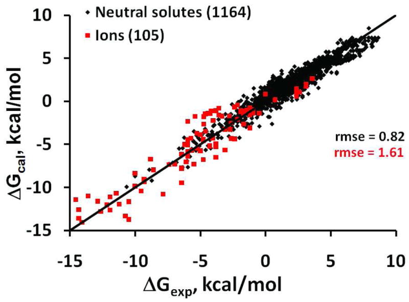
Experimental vs. calculated transfer energies for neutral solutes (black, R2=0.92) and ions (red, R2=0.87) obtained with the universal model.
Our model is less accurate for ions, with rmse of 1.61 kcal/mol, although a more rigorous comparison with other models would require a bigger dataset. Our model is universal because it allows calculation of parameters σI and η for any solvent-water system using solvent polarity descriptors and regression coefficients determined here (Table 5, equation 11). Hence, the model can be applied for the evaluation of transfer energy of molecules between any liquid media. Several validation tests demonstrated the predictive power of the method for molecules of different chemical structure and size and for large set of solvents. Importantly, values of empirical solvation parameters calculated for each solvent-water pair do not depend on the training set used for parameterization. Interestingly, though our previous implicit solvent model developed for simulations of proteins in membranes3 was oversimplified and parameterized on a much smaller dataset, the underlying atomic solvation parameters for five most common atom types (Csp3, Csp2, O, N/HN, OH) are close in both current and previous models (see 2nd and 10th columns in Table 6).
All parameters of the model are transferrable from small organic compounds to biological macromolecules composed of the same types of atoms. However, the simulation of proteins in membranes requires the prior knowledge of polarity descriptors that change along the bilayer normal (z). The required polarity profiles, ε(z), π*(z), a(z) and β(z), can be obtained either experimentally using different spectroscopic probes4–9 or theoretically from the lipid fragment distributions along the bilayer normal105 and group constants of the lipid fragments106, as described in the following paper.
CONCLUSIONS
We have developed a new implicit solvation model that can be applied for calculating transfer energies of neutral molecules and ions from water to environments with defined bulk properties, such as dielectric constant (ε), dipolar/polarizability parameter (π*) and hydrogen and hydrogen bonding acidity (α) and basicity (β) parameters of Abraham. The model is relatively simple, as it includes a small set of empirical parameters and several linear equations. The accuracy of the model in calculation of transfer free energies of neutral molecules is comparable with the most advanced solvation models. This model satisfies three essential criteria: it is universal, physics-based and computationally efficient. The computational efficiency of the method allows application of the model to large-scale computational analyses of small organic compounds or biological macromolecules. It can be readily used for prediction of ADMET properties of drugs by calculating partition coefficients of molecules between water and any isotropic solvent with defined bulk properties. More importantly, the universal model can describe solvation of molecules in anisotropic environment, such as artificial phospholipid bilayers or biological membranes. The following paper represents the validated application of this model for prediction of membrane binding affinities and spatial positions in membranes of small molecule and membrane-associated peptides and proteins. The model can be further applied for prediction of membrane permeation of structurally diverse molecules.
Supplementary Material
Acknowledgments
This research was supported by grant 0849713 (A.L., I.P.) from the National Science Foundation (Division of Biological Infrastructure), Upjohn award from the College of Pharmacy of the University of Michigan (A.L.) and in part by the grant 5R01DA003910-23 (H.I.M.) from the National Institute of Health (National Institute Of Drug Abuse). We are thankful to Dr. Hubbard for the kindly provided NACCESS program.
ABBREVIATIONS
- ASA
solvent accessible-surface area
- MD
Molecular Dynamics
- QSAR
Quantitative Structure Activity Relationship
- LSER
Linear Solvation Energy Relationship
- vdW
van der Waals
- CHX
cyclohexane
- HDC
hydrocarbon
- DEE
diethylether
- DBE
dibutylether
- OCT
octanol
- BNZ
benzene
- CHL
chloroform
- DCE
1,2-dichloroethane
- DCD
1,9-decadiene
- BTA
butyl acetate
- MeOH
methanol
- EtOH
ethanol
- PrOH
propanol
- BuOH
butanol
- DMF
dimethylformamide
- MeCN
acetonitrile
- DMSO
dimethyl sulfoxide
- Me2CO
aceton
- MPA
methyl-phenyl-acethyl
- CMPA
carboxymethyl-phenyl-acetyl
- A
alanyl, Sar-sarcosyl
- G
glycyl
- Tol
p-toluyl
- MPHA
p-methyl-hippuric acid
Footnotes
Supporting Information Available: Empirical polarity parameters of 20 solvents (Table S1), experimental transfer energies of neutral compounds from solvents to water (Tables S2, S3) and from vapor to solvents (Table S4), transfer free energies of ions from solvents to water (Table S5), atomic solvation parameters obtained for transfer from solvents to water and from vapor to water using alternative dielectric models (Tables S6-S9), and linear regression coefficients of atomic solvation parameters obtained using an alternative dataset (Table S10) or an alternative dielectric model (Table S11) are available as Supporting Information. This material is available free of charge via the Internet at http://pubs.acs.org.
Contributor Information
Andrei L. Lomize, Email: almz@umich.edu.
Irina Pogozheva, Email: irinap@umich.edu.
Henry I Mosberg, Email: him@umich.edu.
References
- 1.Feig M, Brooks CL. Recent advances in the development and application of implicit solvent models in biomolecule simulations. Curr Opin Struct Biol. 2004;14:217–224. doi: 10.1016/j.sbi.2004.03.009. [DOI] [PubMed] [Google Scholar]
- 2.Grossfield A. Implicit modeling of membranes. In: Feller SE, editor. Curents Topics in Membranes. Computational Modeling of Membrane Bilayers. Vol. 60. Academic Press; 2008. pp. 131–157. [Google Scholar]
- 3.Lomize AL, Pogozheva ID, Lomize MA, Mosberg HI. Positioning of proteins in membranes: A computational approach. Protein Sci. 2006;15:1318–1333. doi: 10.1110/ps.062126106. [DOI] [PMC free article] [PubMed] [Google Scholar]
- 4.Cohen Y, Afri M, Frimer AA. NMR-based molecular ruler for determining the depth of intercalants within the lipid bilayer Part II. The preparation of a molecular ruler. Chem Phys Lipids. 2008;155:114–119. doi: 10.1016/j.chemphyslip.2008.07.007. [DOI] [PubMed] [Google Scholar]
- 5.Marsh D. Membrane water-penetration profiles from spin labels. Eur Biophys J Biophy. 2002;31:559–562. doi: 10.1007/s00249-002-0245-z. [DOI] [PubMed] [Google Scholar]
- 6.Marsh D. Reaction fields and solvent dependence of the EPR parameters of nitroxides: The microenvironment of spin labels. J Magn Reson. 2008;190:60–67. doi: 10.1016/j.jmr.2007.10.004. [DOI] [PubMed] [Google Scholar]
- 7.Koehorst RBM, Spruijt RB, Hemminga MA. Site-directed fluorescence labeling of a membrane protein with BADAN: Probing protein topology and local environment. Biophys J. 2008;94:3945–3955. doi: 10.1529/biophysj.107.125807. [DOI] [PMC free article] [PubMed] [Google Scholar]
- 8.Carrozzino JM, Fuguet E, Helburn R, Khaledi MG. Characterization of small unilamellar vesicles using solvatochromic pi* indicators and particle sizing. J Biochem Biophys Methods. 2004;60:97–115. doi: 10.1016/j.jbbm.2004.04.014. [DOI] [PubMed] [Google Scholar]
- 9.Prosser RS, Luchette PA, Westerman PW. Using O-2 to probe membrane immersion depth by F-19 NMR. Proc Natl Acad Sci US A. 2000;97:9967–9971. doi: 10.1073/pnas.170295297. [DOI] [PMC free article] [PubMed] [Google Scholar]
- 10.Giesen DJ, Hawkins GD, Liotard DA, Cramer CJ, Truhlar DG. A universal model for the quantum mechanical calculation of free energies of solvation in non-aqueous solvents. Theor Chem Acc. 1997;98:85–109. [Google Scholar]
- 11.Torrens F, Sanchez-Marin J, Nebot-Gil I. Universal model for the calculation of all organic solvent-water partition coefficients. J Chromatogr A. 1998;827:345–358. [Google Scholar]
- 12.Ruelle P. Universal model based on the mobile order and disorder theory for predicting lipophilicity and partition coefficients in all mutually immiscible two- phase liquid systems. J Chem Inf Comput Sci. 2000;40:681–700. doi: 10.1021/ci9902752. [DOI] [PubMed] [Google Scholar]
- 13.Tomasi J, Persico M. Molecular-Interactions In Solution - An Overview Of Methods Based On Continuous Distributions Of The Solvent. Chem Rev. 1994;94:2027–2094. [Google Scholar]
- 14.Cramer CJ, Truhlar DG. Implicit solvation models: Equilibria, structure, spectra, and dynamics. Chem Rev. 1999;99:2161–2200. doi: 10.1021/cr960149m. [DOI] [PubMed] [Google Scholar]
- 15.Orozco M, Luque FJ. Theoretical methods for the description of the solvent effect in biomolecular systems. Chem Rev. 2000;100:4187–4225. doi: 10.1021/cr990052a. [DOI] [PubMed] [Google Scholar]
- 16.Gumbart J, Wang Y, Aksimentiev A, Tajkhorshid E, Schulten K. Molecular dynamics simulations of proteins in lipid bilayers. Curr Opin Struct Biol. 2005;15:423–431. doi: 10.1016/j.sbi.2005.07.007. [DOI] [PMC free article] [PubMed] [Google Scholar]
- 17.Sansom MSP, Scott KA, Bond PJ. Coarse-grained simulation: a high-throughput computational approach to membrane proteins. Biochem Soc Trans. 2008;36:27–32. doi: 10.1042/BST0360027. [DOI] [PubMed] [Google Scholar]
- 18.Halgren TA, Damm W. Polarizable force fields. Curr Opin Struct Biol. 2001;11:236–242. doi: 10.1016/s0959-440x(00)00196-2. [DOI] [PubMed] [Google Scholar]
- 19.Ponder JW, Case DA. Force fields for protein simulations. Adv Protein Chem. 2003;66:27–85. doi: 10.1016/s0065-3233(03)66002-x. [DOI] [PubMed] [Google Scholar]
- 20.Israelachvili JN. Intermolecular and surface forces: with applications to colloidal and biological systems. Academic Press; London; Orlando, USA: 1985. p. 296. [Google Scholar]
- 21.Lazaridis T, Archontis G, Karplus M. Enthalpic contribution to protein stability: Insights from atom-based calculations and statistical mechanics. Adv Protein Chem. 1995;47:231–306. doi: 10.1016/s0065-3233(08)60547-1. [DOI] [PubMed] [Google Scholar]
- 22.Kollman P. Free-energy calculations - applications to chemical and biochemical phenomena. Chem Rev. 1993;93:2395–2417. [Google Scholar]
- 23.Cramer CJ, Truhlar DG. A universal approach to solvation modeling. Acc Chem Res. 2008;41:760–768. doi: 10.1021/ar800019z. [DOI] [PubMed] [Google Scholar]
- 24.Bordner AJ, Cavasotto CN, Abagyan RA. Accurate transferable model for water, n-octanol, and n-hexadecane solvation free energies. J Phys Chem B. 2002;106:11009–11015. [Google Scholar]
- 25.Tropsha A. Best Practices for QSAR Model Development, Validation, and Exploitation. Mol Inf. 2010;29:476–488. doi: 10.1002/minf.201000061. [DOI] [PubMed] [Google Scholar]
- 26.Carrupt PA, Testa B, Gaillard P. Computational Approaches to Lipophilicity: Methods and Applications. In: Lipkowitz KB, Boyd DB, editors. Reviews in Computational Chemistry. Vol. 11. Wiley-VCH, John Wiley and Sons, Inc; New York: 1997. pp. 241–315. [Google Scholar]
- 27.Eisenberg D, McLachlan AD. Solvation energy in protein folding and binding. Nature (London) 1986;319:199–203. doi: 10.1038/319199a0. [DOI] [PubMed] [Google Scholar]
- 28.Ducarme P, Rahman M, Brasseur R. IMPALA: A simple restraint field to simulate the biological membrane in molecular structure studies. Proteins. 1998;30:357–371. [PubMed] [Google Scholar]
- 29.Efremov RG, Nolde DE, Vergoten G, Arseniev AS. A solvent model for simulations of peptides in bilayers. I. Membrane-promoting alpha-helix formation. Biophys J. 1999;76:2448–2459. doi: 10.1016/S0006-3495(99)77400-X. [DOI] [PMC free article] [PubMed] [Google Scholar]
- 30.Lazaridis T. Implicit solvent simulations of peptide interactions with anionic lipid membranes. Proteins. 2005;58:518–527. doi: 10.1002/prot.20358. [DOI] [PubMed] [Google Scholar]
- 31.Lazaridis T, Mallik B, Chen Y. Implicit solvent simulations of DPC micelle formation. J Phys Chem B. 2005;109:15098–15106. doi: 10.1021/jp0516801. [DOI] [PubMed] [Google Scholar]
- 32.Lomize MA, Lomize AL, Pogozheva ID, Mosberg HI. OPM: Orientations of proteins in membranes database. Bioinformatics. 2006;22:623–625. doi: 10.1093/bioinformatics/btk023. [DOI] [PubMed] [Google Scholar]
- 33.Lomize AL, Pogozheva ID, Lomize MA, Mosberg HI. The role of hydrophobic interactions in positioning of peripheral proteins in membranes. BMC Struct Biol. 2007;7:44. doi: 10.1186/1472-6807-7-44. [DOI] [PMC free article] [PubMed] [Google Scholar]
- 34.Sitkoff D, Sharp KA, Honig B. Accurate calculation of hydration free-energies using macroscopic solvent models. J Phys Chem. 1994;98:1978–1988. [Google Scholar]
- 35.Chen J, Brooks CL. Implicit modeling of nonpolar solvation for simulating protein folding and conformational transitions. Phys Chem Chem Phys. 2008;10:471–481. doi: 10.1039/b714141f. [DOI] [PubMed] [Google Scholar]
- 36.Tanizaki S, Feig M. Molecular dynamics simulations of large integral membrane proteins with an implicit membrane model. J Phys Chem B. 2006;110:548–556. doi: 10.1021/jp054694f. [DOI] [PubMed] [Google Scholar]
- 37.Ulmschneider MB, Ulmschneider JP, Sansom MSP, Di Nola A. A generalized Born implicit-membrane representation compared to experimental insertion free energies. Biophys J. 2007;92:2338–2349. doi: 10.1529/biophysj.106.081810. [DOI] [PMC free article] [PubMed] [Google Scholar]
- 38.Reichardt C. Solvents and solvent effects: An introduction. Org Process Res Dev. 2007;11:105–113. [Google Scholar]
- 39.Abraham MH. Hydrogen-bonding.31. Construction of a scale of solute effective or summation hydrogen-bond basicity. J Phys Org Chem. 1993;6:660–684. [Google Scholar]
- 40.Abraham MH. Scales of solute hydrogen-bonding - their construction and application to physicochemical and biochemical processes. Chem Soc Rev. 1993;22:73–83. [Google Scholar]
- 41.Laurence C, Berthelot M. Observations on the strength of hydrogen bonding. Perspect Drug Discov. 2000;18:39–60. [Google Scholar]
- 42.Hunter CA. Quantifying intermolecular interactions: Guidelines for the molecular recognition toolbox. Angew Chem, Int Ed. 2004;43:5310–5324. doi: 10.1002/anie.200301739. [DOI] [PubMed] [Google Scholar]
- 43.Marcus Y. The properties of organic liquids that are relevant to their use as solvating solvents. Chem Soc Rev. 1993;22:409–416. [Google Scholar]
- 44.Laurence C, Nicolet P, Dalati MT, Abboud JLM, Notario R. The empirical-treatment of solvent solute interactions - 15 years of PI. J of Phys Chem. 1994;98:5807–5816. [Google Scholar]
- 45.Marcus Y. Some thermodynamic aspects of ion transfer. Electrochim Acta. 1998;44:91–98. [Google Scholar]
- 46.Chambers CC, Giesen DJ, Hawkins GD, Cramer CJ, Truhlar DG, Vaes WHJ. Modeling the effect of solvation on structure, reactivity, and partitioning of organic solutes: Utility in drug design. In: Truhlar DG, Howe WJ, Hopfinger AJ, Blaney J, Dammkoehler RA, editors. Rational Drug Design. Vol. 108. Springer; New York: 1999. pp. 51–72. [Google Scholar]
- 47.Block H, Walker SM. Modification of Onsager theory for a dielectric. Chem Phys Lett. 1973;19:363–364. [Google Scholar]
- 48.Abe T. A modification of the Born equation. J Phys Chem. 1986;90:713–715. [Google Scholar]
- 49.Hubbard SJ, Thornton JM. NACCESS computer program. Department of Biochemistry and Molecular Biology, University College London; London, UK: 1993. [Google Scholar]
- 50.Rowland RS, Taylor R. Intermolecular nonbonded contact distances in organic crystal structures: Comparison with distances expected from van der Waals radii. J Phys Chem. 1996;100:7384–7391. [Google Scholar]
- 51.Baes CF, Moyer BA. Solubility parameters and the distribution of ions to nonaqueous solvents. J Phys Chem B. 1997;101:6566–6574. [Google Scholar]
- 52.Tsai J, Taylor R, Chothia C, Gerstein M. The packing density in proteins: Standard radii and volumes. J Mol Biol. 1999;290:253–266. doi: 10.1006/jmbi.1999.2829. [DOI] [PubMed] [Google Scholar]
- 53.Rekker RF, Mannhold R, Bijloo G, de Vries G, Dross K. The lipophilic behaviour of organic compounds: 2. The development of an aliphatic hydrocarbon/water fragmental system via interconnection with octanol-water partitioning data. Quant Struct-Act Rel. 1998;17:537–548. [Google Scholar]
- 54.Winget PD, DM, Giesen DJ, Cramer CJ, Truhlar DG. [accessed Jan 15, 2009];Minnesota Solvent Descriptor Database. http://comp.chem.umn.edu/solvation/mnsddb.pdf.
- 55.Abboud JLM, Notario R. Critical compilation of scales of solvent parameters. Part I. Pure, non-hydrogen bond donor solvents - Technical report. Pure Appl Chem. 1999;71:645–718. [Google Scholar]
- 56.Gee N, Shinsaka K, Dodelet JP, Freeman GR. Dielectric-constant against temperature for 43 liquids. J Chem Thermodyn. 1986;18:221–234. [Google Scholar]
- 57.Shih P, Pedersen LG, Gibbs PR, Wolfenden R. Hydrophobicities of the nucleic acid bases: Distribution coefficients from water to cyclohexane. J Mol Biol. 1998;280:421–430. doi: 10.1006/jmbi.1998.1880. [DOI] [PubMed] [Google Scholar]
- 58.Radzicka A, Wolfenden R. Comparing the polarities of the amino-acids - side-chain distribution coefficients between the vapor-phase, cyclohexane, 1-octanol, and neutral aqueous-solution. Biochemistry. 1988;27:1664–1670. [Google Scholar]
- 59.Caron G, Steyaert G, Pagliara A, Reymond F, Crivori P, Gaillard P, Carrupt PA, Avdeef A, Comer J, Box KJ, Girault HH, Testa B. Structure-lipophilicity relationships of neutral and protonated beta-blockers Part I Intra- and intermolecular effects in isotropic solvent systems. Helv Chim Acta. 1999;82:1211–1222. [Google Scholar]
- 60.Reymond F, Carrupt PA, Testa B, Girault HH. Charge and delocalisation effects on the lipophilicity of protonable drugs. Chem-Eur J. 1999;5:39–47. [Google Scholar]
- 61.Reymond F, Chopineaux-Courtois V, Steyaert G, Bouchard G, Carrupt PA, Testa B, Girault HH. Ionic partition diagrams of ionisable drugs: pH-lipophilicity profiles, transfer mechanisms and charge effects on solvation. J Electroanal Chem. 1999;462:235–250. [Google Scholar]
- 62.Cao YC, Xiang TX, Anderson BD. Development of structure-lipid bilayer permeability relationships for peptide-like small organic molecules. Mol Pharm. 2008;5:371–388. doi: 10.1021/mp700100n. [DOI] [PubMed] [Google Scholar]
- 63.Tejwani RW, Anderson BD. Influence of intravesicular pH drift and membrane binding on the liposomal release of a model amine-containing permeant. J Pharm Sci. 2008;97:381–399. doi: 10.1002/jps.21108. [DOI] [PubMed] [Google Scholar]
- 64.Abraham MH, Zissimos AM, Acree WE. Partition of solutes from the gas phase and from water to wet and dry di-n-butyl ether: a linear free energy relationship analysis. Phys Chem Chem Phys. 2001;3:3732–3736. [Google Scholar]
- 65.Abraham MH, Zissimos AM, Acree WE. Partition of solutes into wet and dry ethers; an LFER analysis. New J Chem. 2003;27:1041–1044. [Google Scholar]
- 66.Sprunger LM, Proctor A, Acree WE, Abraham MH, Benjelloun-Dakhama N. Correlation and prediction of partition coefficient between the gas phase and water, and the solvents dry methyl acetate, dry and wet ethyl acetate, and dry and wet butyl acetate. Fluid Phase Equilibr. 2008;270:30–44. [Google Scholar]
- 67.Abraham MH, Platts JA, Hersey A, Leo AJ, Taft RW. Correlation and estimation of gas-chloroform and water-chloroform partition coefficients by a linear free energy relationship method. J Pharm Sci. 1999;88:670–679. doi: 10.1021/js990008a. [DOI] [PubMed] [Google Scholar]
- 68.Ahmed H, Poole CE. Model for the distribution of neutral organic compounds between n-hexane and acetonitrile. J Chromatogr A. 2006;1104:82–90. doi: 10.1016/j.chroma.2005.11.065. [DOI] [PubMed] [Google Scholar]
- 69.Abraham MH, Whiting GS, Carr PW, Ouyang H. Hydrogen bonding. Part 45. The solubility of gases and vapours in methanol at 298 K: An LFER analysis. J Chem Soc, Perk T 2. 1998;6:1385–1390. [Google Scholar]
- 70.Ahmed H, Poole CF. Distribution of neutral organic compounds between n-heptane and methanol or N,N-dimethylformamide. J Sep Sci. 2006;29:2158–2165. doi: 10.1002/jssc.200600131. [DOI] [PubMed] [Google Scholar]
- 71.Abraham MH, Whiting GS, Shuely WJ, Doherty RM. The solubility of gases and vapours in ethanol - the connection between gaseous solubility and water-solvent partition. Can J Chem. 1998;76:703–709. [Google Scholar]
- 72.Abraham MH, Le J, Acree WE, Carr PW. Solubility of gases and vapours in propan-1-ol at 298 K. J Phys Org Chem. 1999;12:675–680. doi: 10.1016/s0045-6535(00)00288-5. [DOI] [PubMed] [Google Scholar]
- 73.Abraham MH, Nasezadeh A, Acree WE. Correlation and prediction of partition coefficients from the gas phase and from water to alkan-1-ols. Ind Eng Chem Res. 2008;47:3990–3995. [Google Scholar]
- 74.Abraham MH, Whiting GS, Doherty RM, Shuely WJ. Hydrogen-bonding.14. The characterization of some n-substituted amides as solvents - comparison with gas-liquid-chromatography stationary phases. J Chem Soc, Perk T 2. 1990;11:1851–1857. [Google Scholar]
- 75.Katritzky AR, Tulp I, Fara DC, Lauria A, Maran U, Acree WE. A general treatment of solubility. 3. Principal component analysis (PCA) of the solubilities of diverse solutes in diverse solvents. J Chem Inf Model. 2005;45:913–923. doi: 10.1021/ci0496189. [DOI] [PubMed] [Google Scholar]
- 76.Abraham MH, Chadha HS, Whiting GS, Mitchell RC. Hydrogen-bonding.32. An analysis of water-octanol and water-alkane partitioning and the delta-logP parameter of seiler. J Pharm Sci. 1994;83:1085–1100. doi: 10.1002/jps.2600830806. [DOI] [PubMed] [Google Scholar]
- 77.Li JB, Zhu TH, Hawkins GD, Winget P, Liotard DA, Cramer CJ, Truhlar DG. Extension of the platform of applicability of the SM5.42R universal solvation model. Theor Chem Acc. 1999;103:9–63. [Google Scholar]
- 78.Wang JM, Wang W, Huo SH, Lee M, Kollman PA. Solvation model based on weighted solvent accessible surface area. J Phys Chem B. 2001;105:5055–5067. [Google Scholar]
- 79.Zissimos AM, Abraham MH, Barker MC, Box KJ, Tam KY. Calculation of Abraham descriptors from solvent-water partition coeffcients in four different systems; evaluation of different methods of calculation. J Chem Soc Perk T 2. 2002;3:470–477. [Google Scholar]
- 80.Zissimos AM, Abraham MH, Du CM, Valko K, Bevan C, Reynolds D, Wood J, Tam KY. Calculation of Abraham descriptors from experimental data from seven HPLC systems; evaluation of five different methods of calculation. J Chem Soc Perk T 2. 2002;12:2001–2010. [Google Scholar]
- 81.Abraham MH, Zhao YH. Determination of solvation descriptors for ionic species: Hydrogen bond acidity and basicity. J Org Chem. 2004;69:4677–4685. doi: 10.1021/jo049766y. [DOI] [PubMed] [Google Scholar]
- 82.Mintz C, Clark M, Acree WE, Abraham MH. Enthalpy of solvation correlations for gaseous solutes dissolved in water and in 1-octanol based on the abraham model. J Chem Inf Model. 2007;47:115–121. doi: 10.1021/ci600402n. [DOI] [PubMed] [Google Scholar]
- 83.Sprunger LM, Gibbs J, Acree WE, Abraham MH. Correlation and prediction of partition coefficients for solute transfer to 1,2-dichloroethane from both water and from the gas phase. Fluid Phase Equilibr. 2008;273:78–86. [Google Scholar]
- 84.Holtzer A. Does Flory-Huggins theory help in interpreting solute partitioning experiments. Biopolymers. 1994;34:315–320. doi: 10.1002/bip.360340303. [DOI] [PubMed] [Google Scholar]
- 85.McClellan AL. Tables of experimental dipole moments. W.H. Freeman and Company; San Francisco and London: 1963. p. 713. [Google Scholar]
- 86.Lien EJ, Guo ZR, Li RL, Su CT. Use of dipole-moment as a parameter in drug receptor interaction and quantitative structure activity relationship studies. J Pharm Sci. 1982;71:641–655. doi: 10.1002/jps.2600710611. [DOI] [PubMed] [Google Scholar]
- 87.Li WY, Guo ZR, Lien EJ. Examination of the interrelationship between aliphatic group dipole-moment and polar substituent constants. J Pharm Sci. 1984;73:553–558. doi: 10.1002/jps.2600730430. [DOI] [PubMed] [Google Scholar]
- 88.Manzur ME, Romano E, Vallejo S, Wesler S, Suvire F, Enriz RD, Molina MAA. Analysis of dielectric properties of cytosine in aqueous solution. J Mol Liq. 2001;94:87–96. [Google Scholar]
- 89.Spackman MA, Munshi P, Dittrich B. Dipole moment enhancement in molecular crystals from X-ray diffraction data. ChemPhysChem. 2007;8:2051–2063. doi: 10.1002/cphc.200700339. [DOI] [PubMed] [Google Scholar]
- 90.Shukla MK, Mishra PC. Excited-state molecular electric properties of some biologically important purines, pyrimidines, and azines: An ab initio study. J Chem Inf Comp Sci. 1998;38:678–684. [Google Scholar]
- 91.Parkanyi C, Boniface C, Aaron JJ, Gaye MD, Vonszentpaly L, Ghosh R, Raghuveer KS. Electronic absorption and fluorescence-spectra and excited singlet-state dipole-moments of biologically important pyrimidines. Struct Chem. 1992;3:277–289. [Google Scholar]
- 92.Demore BB, Wilcox WS, Goldstein JH. Microwave spectrum and dipole moment of pyridine. J Chem Phys. 1954;22:876–877. [Google Scholar]
- 93.Civcir PU. A theoretical study of tautomerism of cytosine, thymine, uracil and their 1-methyl analogues in the gas and aqueous phases using AM1 and PM3. J Mol Struc-Theochem. 2000;532:157–169. [Google Scholar]
- 94.Aaron JJ, Diabou Gaye M, Párkányi C, Cho NS, Von Szentpály L. Experimental and theoretical dipole moments of purines in their ground and lowest excited singlet states. J Mol Struct. 1987;156:119–135. [Google Scholar]
- 95.Schmid R. Recent advances in the description of the structure of water, the hydrophobic effect, and the like-dissolves-like rule. Monatsh Chem. 2001;132:1295–1326. [Google Scholar]
- 96.Solomonov BN, Novikov VB. Solution calorimetry of organic nonelectrolytes as a tool for investigation of intermolecular interactions. J Phys Org Chem. 2008;21:2–13. [Google Scholar]
- 97.Arey JS, Green WH, Gschwend PM. The electrostatic origin of Abraham’s solute polarity parameter. Journal of Physical Chemistry B. 2005;109:7564–7573. doi: 10.1021/jp044525f. [DOI] [PubMed] [Google Scholar]
- 98.Karplus PA. Hydrophobicity regained. Protein Sci. 1997;6:1302–1307. doi: 10.1002/pro.5560060618. [DOI] [PMC free article] [PubMed] [Google Scholar]
- 99.Abboud JLM, Taft RW. Interpretation of a general scale of solvent polarities - simplified reaction field-theory modification. J Phys Chem. 1979;83:412–419. [Google Scholar]
- 100.Abboud JLM, Guiheneuf G, Essfar M, Taft RW, Kamlet MJ. Linear solvation energy relationships.21. Gas-phase data as tools for the study of medium effects. J Phys Chem. 1984;88:4414–4420. [Google Scholar]
- 101.Kamlet MJ, Doherty RM, Taft RW, Abraham MH, Koros WJ. Solubility properties in polymers and biological media.3. Predictional methods for critical-temperatures, boiling points, and solubility properties (RG values) based on molecular-size, polarizability, and dipolarity. J Am Chem Soc. 1984;106:1205–1212. [Google Scholar]
- 102.Meeks OR, Rybolt TR. Correlations of adsorption energies with physical and structural properties of adsorbate molecules. J Colloid Interf Sci. 1997;196:103–109. doi: 10.1006/jcis.1997.5198. [DOI] [PubMed] [Google Scholar]
- 103.Chen XQ, Cho SJ, Li Y, Venkatesh S. Prediction of aqueous solubility of organic compounds using a quantitative structure-property relationship. J Pharm Sci. 2002;91:1838–1852. doi: 10.1002/jps.10178. [DOI] [PubMed] [Google Scholar]
- 104.Baczek T, Kaliszan R, Novotna K, Jandera P. Comparative characteristics of HPLC columns based on quantitative structure-retention relationships (QSRR) and hydrophobic-subtraction model. J Chromatogr A. 2005;1075:109–115. doi: 10.1016/j.chroma.2005.03.117. [DOI] [PubMed] [Google Scholar]
- 105.Kucerka N, Nagle JF, Sachs JN, Feller SE, Pencer J, Jackson A, Katsaras J. Lipid bilayer structure determined by the simultaneous analysis of neutron and x-ray scattering data. Biophys J. 2008;95:2356–2367. doi: 10.1529/biophysj.108.132662. [DOI] [PMC free article] [PubMed] [Google Scholar]
- 106.Abraham MH, Platts JA. Hydrogen bond structural group constants. J Org Chem. 2001;66:3484–3491. doi: 10.1021/jo001765s. [DOI] [PubMed] [Google Scholar]
Associated Data
This section collects any data citations, data availability statements, or supplementary materials included in this article.