Raster image correlation spectroscopy in live cells

Abstract

Raster image correlation spectroscopy (RICS) is a noninvasive technique to detect and quantify events in a live cell, including concentration of molecules and diffusion coefficients of molecules; in addition, by measuring changes in diffusion coefficients, RICS can indirectly detect binding. Any specimen containing fluorophores that can be imaged with a laser scanning microscope can be analyzed using RICS. There are other techniques to measure diffusion coefficients and binding; however, RICS fills a unique niche. It provides spatial information and can be performed in live cells using a conventional confocal microscope. It can measure a range of diffusion coefficients that is not accessible with any other single optical correlation–based technique. In this article we describe a protocol to obtain raster scanned images with an Olympus FluoView FV1000 confocal laser scanning microscope using Olympus FluoView software to acquire data and SimFCS software to perform RICS analysis. Each RICS measurement takes several minutes. The entire procedure can be completed in ~2 h. This procedure includes focal volume calibration using a solution of fluorophores with a known diffusion coefficient and measurement of the diffusion coefficients of cytosolic enhanced green fluorescent protein (EGFP) and EGFP-paxillin.

INTRODUCTION

Raster image correlation spectroscopy (RICS) is a noninvasive image analysis technique to measure the diffusion coefficient and concentration of fluorescently labeled proteins in cells^1,2. Molecular dynamics on time scales ranging from microseconds to milliseconds can be measured by RICS by adjusting the sample rate (pixel dwell time). This means that both quickly moving cytosolic proteins and slower membrane-bound proteins can be studied with RICS. Originally developed by Digman et al.¹, RICS is accessible to many researchers because it can be performed using a commercially available laser scanning microscope.

Basic theory

RICS analysis must be performed on images acquired through raster scanning. Laser scanning microscopes generate images by measuring fluorescence intensity across an area one pixel at a time (a ‘pixel’ in this context does not have the same definition as a pixel in computer graphics, but rather refers to a localized intensity measurement). The value of a pixel is obtained by illuminating a region of the sample with the focal volume of a laser beam and measuring the intensity of the emitted fluorescence. The laser beam is then moved to a new location and a new pixel is recorded. Each pixel can be considered to correspond to a region of the sample, with its width (called the pixel size) defined by the distance the beam moves between measurements. This means that the size of a pixel is separate and independent from the size of the focal volume of the laser beam^3,4.

The ‘raster’ in RICS refers to the order in which these pixels are collected to generate an image. The top left pixel is measured first. Thereafter, the top row of pixels is collected from left to right. The laser then travels back to the left of the image without collecting any pixels and begins a second row. Rows are collected in this manner from top to bottom until an entire image is obtained. This is the same pattern of raster scanning used in cathode ray tube monitors. Because each pixel is collected at a different time, there is temporal information included in each individual image. This is referred to as the ‘hidden time structure’ and can be used to extract temporal information from the image^1,2.

Diffusion coefficient and concentration information is extracted from raster scanned images using RICS analysis. There are two steps in RICS analysis: background subtraction and image correlation. Background subtraction removes stationary or slowly moving objects from the image. At its most basic, background subtraction subtracts the average of all images from each image. However, cells usually do not remain completely stationary during the time it takes to acquire a series of images. To account for this, and to remove slow-moving objects, moving average background subtraction is used. In moving average background subtraction, the average of a range of consecutive images is subtracted from the image in the middle of this range. For example, if moving average subtraction is performed using 10 frames, the average of frames 1–10 is subtracted from frame 5.

After stationary and slow-moving objects are removed with background subtraction, image autocorrelation is calculated on each image using equation 1 (refs. 1,2,5–7)

$$G(\xi ,\psi )=\frac{{\langle \delta i(x,y)\delta i(x+\xi ,y+\psi )\rangle }_{x,y}}{{\langle i(x,y)\rangle }_{x,y}{\langle i(x,y)\rangle }_{x,y}}$$ (1)

where i(x, y) is the intensity at each pixel of the image, ξ and ψ are the x and y spatial correlation shifts and δ(i) = i − 〈i〉 and 〈…〉_x,y is the spatial average of the image. Computational speed can be improved by calculating the image correlation with fast Fourier transforms, as is done by the software described here.

The image correlations of all the frames are averaged and the result is fit with an equation relating the correlation to the diffusion coefficient and particle concentration. Equation 2 is the most basic form of this function and the one used in the examples presented here^1,2. Variations on this equation that account for factors such as two-photon excitation and membrane-bound diffusion are described elsewhere^1,8.

$$\begin{array}{l}{G}_{\text{RICS}}(\xi ,\psi )=S(\xi ,\psi )G(\xi ,\psi )+b\\ G(\xi ,\psi )=\frac{\gamma }{N}{\left(1+\frac{4D({\tau }_{\text{p}}\xi +{\tau }_{\text{l}}\psi )}{{\omega }_0^2}\right)}^{-1}{\left(1+\frac{4D({\tau }_{\text{p}}\xi +{\tau }_{\text{l}}\psi )}{{\omega }_z^2}\right)}^{-1/2}\\ S(\xi ,\psi )=exp(-\frac{\frac{1}{2}\left[{\left(\frac{2\xi {\delta }_{\text{r}}}{{\omega }_0}\right)}^2+{\left(\frac{2\psi {\delta }_{\text{r}}}{{\omega }_0}\right)}^2\right]}{\left(1+\frac{4D({\tau }_{\text{p}}\xi +{\tau }_{\text{l}}\psi )}{{\omega }_0^2}\right)})\end{array}$$ (2)

N is the number of particles in the focal volume; D the diffusion coefficient; τ_p the pixel dwell time; τ_l the time between lines; δ_r the pixel size; ω₀ the beam waist; and b the background. G_RICS(ξ,ψ) is broken up into two parts: G(ξ,ψ), which is related to molecular dynamics, and S(ξ,ψ), which is related to scanning optics.

It should be noted that multiple images are acquired from RICS analysis for two reasons: (i) so that background subtraction can be performed and (ii) to improve the signal-to-noise ratio. Correlation analysis is not performed between images in RICS. This means that all available temporal information comes from within each image.

Related techniques

Alternatives to RICS fall into three categories: in vitro techniques to measure diffusion coefficient, in vitro techniques to detect protein-protein interactions and other in vivo techniques. The first category includes diffusion NMR spectroscopy. Diffusion NMR can measure diffusion coefficients of molecules in solution and in living tissue but generally does not provide subcellular resolution^9,10. This technique also provides accurate, reproducible results, but it cannot be applied to individual cells at this time. Second, in vitro techniques to measure protein-protein interaction include co-immunoprecipitation (Co-IP). Co-IP is a biochemical technique that uses antibodies to precipitate protein complexes out of solution and identifies their components^11,12. Cells are destroyed during Co-IP, and therefore no spatial information can be recovered.

The third category, in vivo techniques for measuring and mapping diffusion coefficients and detecting protein binding, includes other microscopy- and spectroscopy-based systems. Förster resonance energy transfer (FRET) uses energy transfer and resulting changes in fluorescent emissions to detect protein binding¹³. Fluorescence recovery after photobleaching (FRAP) measures diffusion coefficient by selectively bleaching a region of the cell and observing the return of fluorescent particles to that region^14,15. In comparison with RICS, FRAP has limited ability to map diffusion coefficients, as only a few, preselected regions can be measured. Other in vivo techniques are similar to RICS in that they rely on confocal (or two-photon) microscopy and correlation analysis. These techniques include fluorescence correlation spectroscopy (FCS), temporal image correlation spectroscopy (TICS) and cross-correlation–based variations of these techniques^16–18. FCS and TICS can measure binding either indirectly by detecting a change in the diffusion rate or directly by using a fitting function that accounts for binding. This is similar to RICS. As described here, RICS can indirectly measure binding by detecting changes in the diffusion coefficient. RICS can also measure binding directly by using a fitting equation that accounts for binding; however, this application is not described here⁸. In addition to detecting binding, FCS and TICS can distinguish between binding between particles, and binding between a particle and a scaffold (i.e., the cell membrane). RICS can also make this distinction, although this is not discussed here⁸. The most important consideration when deciding between these techniques is the temporal range that they are suited for. For a more detailed discussion of these techniques, see the review by Kolin and Wiseman¹⁹. Table 1 summarizes alternatives to RICS.

TABLE 1.

Comparison of alternative techniques.

Technique	Measures diffusion coefficient?	Measures binding to other particles?	Measures binding to a scaffold?	Detects binding directly?	Makes measurements in live cells?	In vivo application
RICS	Yes	Yes (not discussed here8)	Yes (not discussed here8)	Yes (not discussed here8)	Yes	Small molecules, cytosolic proteins, transmembrane proteins
NMR	Yes	No	No	No	No	Diffusion through tissue, not subcellular measurements
Co-IP	No	Detects interactions	No	No	No	—
FRET	No	Yes	No	No	Yes	Interactions between two labeled proteins
FRAP	Yes	No	No	No	Yes	Protein aggregates, membrane proteins
FCS	Yes	Yes	Yes	Yes	Yes	Small molecules
TICS	Yes	Yes	Yes	Yes	Yes	Large protein aggregates, membrane proteins

Co-IP, co-immunoprecipitation; FRAP, fluorescence recovery after photobleaching; FRET, Forester resonance energy transfer; RICS, raster image correlation spectroscopy; TICS, temporal image correlation spectroscopy.

Applications

RICS has been applied to a range of problems in cell biology. It was originally developed to study the behavior of paxillin in focal adhesions¹. In this application, RICS helped to develop a description of the binding and unbinding behavior of protein aggregates. RICS has been used to identify and quantify diffusion restrictions on ATP in rat cardiomyocytes²⁰. Another application of RICS is the diffusion of lipid analogs in membranes and giant unilamellar vesicles²¹. It has also been used to expand on results from FRAP and western blot experiments in the study of the RAD18 protein after ultraviolet damage²².

Additional RICS techniques and applications

The potential applications and availability of RICS extend beyond what is described here. RICS can be performed on a variety of custom-built and commercial confocal microscope systems, including the Zeiss LSM 510 (Carl Zeiss)²³. The steps included below can also be adapted for other software and optical systems.

RICS can also be applied to a wider variety of biological systems than are described here. For example, this protocol uses a stable cell line, but RICS may work just as well for primary cells. Here the only fluorophore we use is enhanced green fluorescent protein (EGFP), but with appropriate lasers and filters RICS can be applied to other fluorophores as well, as long as the excitation laser, dichroic mirror and emission filter are appropriate for the fluorophore²⁴. It is our intention that readers will apply RICS to their own experiments.

Recent advances in RICS expand on the technique described here. The RICS fitting model can be adapted for more complex situations than simple diffusion. For example, it can account for two distinct populations of diffusing fluorophores²³. Cross-correlation RICS is a recently developed technique that uses two fluorophores to examine protein-protein interaction in more detail²⁴. As mentioned above, RICS can also directly measure binding both to a scaffold and between particles by using a fitting function that accounts for binding⁸.

Experimental design

Instrumentation

RICS requires a confocal microscope to acquire a series of images. A high-numerical-aperture (NA) objective is required to obtain the correct-sized focal volume. Oil immersion, water immersion or air objectives can be used. The objective power should be between ×40 and ×100. The microscope must have a laser with the correct wavelength to excite the fluorophore used in the experiment. There must also be a band-pass filter and dichroic mirror appropriate for the fluorophore.

The selection of a detector requires some discussion. Either an avalanche photodiode or a photomultiplier tube can be used for RICS experiments. In both cases, photon-counting detectors are preferable because they have better rejection of noise. There is an important limitation of these detectors: analog detectors can have spatial correlation between pixels, particularly at short pixel dwell times. To account for this, we recommend skipping pixels when fitting the correlated data (SimFCS has an option to skip pixels). The number of pixels to skip must be determined for each microscope. We recommend taking a series of images under the same conditions as will be used for RICS using a sample that will not fluctuate over time. This can be either a source of constant fluorescence such as the Fluor-o-4 Slide Set (Chroma Technology Group) or a measurement of dark counts. The horizontal width of the image correlation is equal to the number of pixels that need to be skipped when fitting RICS data. The number of pixels to be skipped will be different for each pixel dwell time but only needs to be measured once for a microscope. Alternatively, the same procedure can be used to determine the shortest pixel dwell time that does not produce image correlation.

Data acquisition

Table 2 summarizes the important parameters for acquiring RICS data. On the Olympus FluoView, these parameters are set in the software that controls the microscope, as is described in more detail below.

TABLE 2.

Important parameters for RICS acquisition.

Parameter	Range of values
Pixel dwell time	8–20 μs
Pixel size	≤0.05 μm
Magnification	40× or 100×
NA	≥0.8
Number of images	≥10, usually 50–100
Image size	256 × 256 pixels (recommended)

NA, numerical aperture.

Pixel size is an important consideration in designing an RICS experiment. Again, it should be noted that pixel size is different from focal volume. The focal volume is determined by the optics of the system. Focal volume can be altered by changing the pinhole diameter, but its exact size must be calibrated to perform an accurate RICS measurement. Pixel size is defined by the distance the laser beam travels between collecting pixels. In RICS, the pixel size must be 4–5 times smaller than the focal volume. This means that each pixel in the image is the average intensity in a focal volume that overlaps with the focal volume from neighboring pixels.

On the Olympus FluoView microscopes, pixel size is set with the ‘zoom’ slider. Zooming in gives smaller pixels and zooming out gives larger ones. Pixel size can range from 0.02 μm to 0.06 μm. Setting the pixel size with the zoom slider is described in more detail in the PROCEDURE section.

RICS can measure diffusion coefficients ranging approximately from 0.1 to 1,000 μm² s⁻¹. The pixel dwell time must be appropriate for the diffusion coefficient being measured. The laser needs to move from location to location before, on average, a particle will move out of the pixel. Equation 3 describes the maximum value for τ_p

$${\tau }_{\text{p}}<\frac{{\omega }_0^2}{4D}$$ (3)

Another important consideration in RICS analysis is the number of frames to be used for moving-average background subtraction. Large features should not move by more than one pixel over the frames averaged. This can be estimated with equation 4

$$n<\frac{{\delta }_{\text{r}}}{v{\tau }_{\text{p}}},$$ (4)

where n is the number of frames averaged and v the velocity of the background feature (i.e., the cell), τ_p is the pixel dwell time and δ_r is the pixel size.

RICS can distinguish between multiple events occurring within a cell, such as diffusion of molecules, binding processes and cellular movement. However, the scan speed of the laser must be faster than the movement of the target fluorophore to show correlation between pixels. Therefore, selecting an appropriate pixel dwell time is important for accurate RICS measurements. The approximate diffusion coefficient must be known and taken into account. Like any measurement technique, RICS is only accurate over a certain range. It will not work for processes that are very slow (i.e., seconds timescale) and thus cannot show correlation between pixels of one frame.

Analysis software

There are several software options for analyzing RICS data. SimFCS performs RICS analysis, as described here, as well as a variety of other correlation-based data analysis routines. SimFCS can also be used for data acquisition. An RICS analysis plug-in for ImageJ and an RICS analysis program for MATLAB are available from the Cell Migration Gateway (Cell Migration Consortium). Zeiss ZEN software has an optional module available for RICS (Carl Zeiss). At the time of the writing of this article, Olympus had a demo version of a RICS analysis package available for Fluoview1000 software.

Biological system

RICS works well on samples that can be imaged easily with confocal microscopy, such as adherent cell lines transfected with or stably expressing fluorescent proteins²⁵. Primary cells stably expressing fluorescent proteins may also be suitable. Appropriate fluorophores should be chosen that are generally bright and photostable so as to increase the signal-to-noise ratio and decrease photobleaching²⁶. Cell lines must be sufficiently robust to withstand heat from the laser and must be large enough (~50 μm wide) to fill a confocal image partially. These cells should be grown in glass-bottom imaging dishes. Before imaging, the cell medium should be changed to a phenol red–free solution, as phenol red will fluoresce when illuminated and can interfere with the measurement.

Controls

Controls will depend on the exact nature of the RICS experiment performed. Calibration can be confirmed by measuring the diffusion coefficient of a second fluorophore in solution. Diffusion coefficient measurements in cells can be confirmed with one of the alternate techniques described above.

Experiments described here

In this article, we describe how to perform RICS calibration and measurements with the commercially available Olympus FluoView FV1000 confocal laser scanning microscope using Olympus FluoView software to acquire data and SimFCS software to analyze the results. Some of the symbols used in the SimFCS software are different from the symbols used here and in other reports. Table 3 compares the print symbols with the symbols used in SimFCS.

TABLE 3.

Comparison of symbols.

Description	Symbol	SimFCS symbol
Beam waist	ω0	Wo
Magnitude of correlation fit at origin	GRICS(0)	G1(0)
Diffusion coefficient	D	D1
Pixel dwell time	τp	Pixel time
Pixel size/distance between pixels	δr	Pixel size
Region of interest		ROI

The first step in any RICS measurement is to calibrate the focal volume of the laser beam waist^1,27. All RICS measurements are dependent on an accurately known focal volume so that the average rate of fluctuation can be accurately related to a diffusion coefficient. The calibration is performed using a fluorophore in solution with a known diffusion coefficient, EGFP in this case. Calibration needs to be repeated each day or whenever the power or wavelength of the laser is changed.

EGFP used for calibration was purified from a culture of BL21DE3 Escherichia coli cells and resuspended in 20 mM Tris buffer (pH 7.4). The concentration of the stock solution was determined with a spectrophotometer at 480 nm and aliquots of the stock were stored at −20 °C. For the experiment, an aliquot was thawed at 4 °C and diluted 1:500 in 20 mM Tris buffer (pH 7.4). The diluted EGFP solution was kept on ice to prevent protein degradation or aggregation before measurement.

The procedures for two example RICS measurements are also described here: RICS in cytosolic EGFP CHO-K1 cells and in EGFP-paxillin CHO-K1 cells²⁸. The procedure is similar to RICS in solution, but care must be taken to keep the cell in focus and in the field of view. In addition, the pixel dwell time must account for a slower diffusion time. Measurements with EGFP and EGFP-paxillin are similar, but the expected results are different. In the case of cytosolic EGFP, RICS can be used to measure the diffusion coefficient of EGFP in the cytosol, which is slower than that of EGFP in solution. In the case of EGFP-paxillin, the diffusion coefficient and concentration of EGFP-paxillin are different in focal adhesions than in the cytosol. RICS analysis performed on different regions of the cell will reflect this.

The cells for these measurements were prepared as follows: 1 week before experiment, CHO-K1 cell lines stably expressing EGFP and EGFP-paxillin were defrosted and cultured in full medium, with geneticin (G418 sulfate) added to select for EGFP-expressing cells. Cells were grown to ~80% confluency in flasks before passaging (about 2 d). On the day of the experiment, approximately 4 h before imaging, the two cell lines were each plated for ~50% confluency in 35-mm imaging dishes coated with 2 μg ml⁻¹ fibronectin.

MATERIALS

REAGENTS

• Calibration fluorophore (40-nm EGFP; BioVision, cat. no. 4999-100)

  ▴ CRITICAL A different fluorophore can be used, as long as the diffusion coefficient is known and the appropriate lasers and filters are available.

• Tris buffer (20 mM, pH 7.4; Fisher Reagents, cat. no. BP152-1)

• Dulbecco’s modified Eagle’s medium (low glucose 1×; Gibco/Invitrogen, cat. no. 0930119DJ) ▴ CRITICAL The medium should not contain phenol red.

• Fetal bovine serum (Sigma-Aldrich, cat. no. F6178)

• Penicillin-streptomycin (Sigma-Aldrich, cat. no. P0781)

• Nonessential amino acid solution (100×; Sigma-Aldrich, cat. no. M7145)

• Geneticin (G418 sulfate; Gibco/Invitrogen, cat. no. 11811-031)

• Cultured CHO-K1 cells (ATCC, cat. no. CCL-61) ▴ CRITICAL Different cultured cells or primary cell lines can be used if desired.

• EGFP vector (BioVision, cat. no. 4999-100) ▴ CRITICAL A different fluorescent protein vector can be used if desired.

EQUIPMENT

• Vibration-isolated optics table

• Olympus FluoView FV1000 ▴ CRITICAL A different confocal laser scanning microscope can be used as described in the Experimental design section.

• Mercury arc lamp ! CAUTION Use eye protection when working with UV light sources.

• Water immersion objective lens (×60, 1.20 NA) ▴ CRITICAL A different high-NA objective can be used as described in the Experimental design section. Oil immersion or air objectives can also be used if the NA is at least 1.1.

• Ultrapure water for immersion objective lens ▴ CRITICAL Use water only on water immersion objectives.

• Ar ion laser at 488 nm (Melles Griot) ▴ CRITICAL A different excitation laser can be used. The laser and filters must be selected for the chosen fluorophores ! CAUTION Use eye protection when working with lasers.

• Dichroic mirror (Chroma Technologies, cat. no. DM405/488) ▴ CRITICAL A different dichroic mirror can be used to separate fluorescence and laser excitation. It must be chosen along with the laser and band-pass filters to match the fluorophore.

• Band-pass filters (Chroma Technologies, cat. no. BA505-540) ▴ CRITICAL A different band-pass filer can be used. It must be chosen along with the laser and dichroic mirror for the selected fluorophores.

• Glass-bottom culture dishes with number 1.5 (0.16–0.19 mm thick) glass (MatTek, cat. no. P35G-1.5-14-C)

• Cover glass (Number 1.5 (0.16–0.19 mm thick); Fisher, cat. no. 22-050-235)

  ▴ CRITICAL The cover glass and glass-bottom coverslip must have the same thickness so that the focal volume will be the same in the calibration and the measurement.

• Photomultiplier tube ▴ CRITICAL A different detector can be used as described in the Experimental design section.

• Olympus FluoView 1.7a ▴ CRITICAL Different software to control microscope, lasers and detectors can be used as described in the Experimental design section.

• SimFCS software (The Laboratory for Fluorescence Dynamics; available at http://www.lfd.uci.edu)

• ▴ CRITICAL Different software for data analysis can be used as described in the Experimental design section.

• ImageJ software (National Institute of Health)

REAGENT SETUP

• Phenol red–free cell growth medium Prepare phenol red–free cell growth medium for imaging by combining low-glucose 1× Dulbecco’s modified Eagle’s medium with 10% (vol/vol) fetal bovine serum, 1% penicillin-streptomycin, 1% nonessential amino acid solution 100×. Approximately 2 ml of medium is needed for each glass-bottom culture dish. Medium can be stored for up to 2 months at 4 °C in a sterile bottle.

• Cell growth Grow cells in the glass-bottom culture dishes as described in reference 29. Before imaging, the growth medium should be exchanged for phenol red–free medium.

• Cell transfection Transfect cells to express fluorescent proteins as described in reference 30.

EQUIPMENT SETUP

The microscope and associated optics should be set up to acquire confocal laser scanning images. A detailed discussion of confocal microscopy can be found in reference 3.

PROCEDURE

Setup ● TIMING 30 min

• 1Turn on the laser, lamp, microscope and computer associated with the microscope.
• 2Select the appropriate laser, dichroic and band-pass filter using the microscope control software. For Olympus FV1000, this can be carried out by selecting EGFP from the ‘DyeList’. Figure 1 shows the appropriate settings in the Olympus FluoView software ‘LightPath & Dyes’ window.
• 3Select the ×60 water objective (Fig. 2, circle 1).

Figure 1.

LightPath & Dyes window in Olympus FluoView 1.7a. EGFP has been selected from the DyeList (circled) and the laser, dichroic mirror (excitation DM) and band-pass filter (BF) have been set automatically. Note that the optical path (yellow) line will change depending on whether the system is set up for laser scanning or for observation through the eyepieces.

Figure 2.

The Acquisition Settings window in Olympus FluoView 1.7a. This window is used to select the objective and to set scan mode, pixel dwell time, pixel size, frame size and image size. Circle 1 shows the button to select the objective. Circle 2 shows the slider to set the pixel dwell time. Circle 3 shows a slider to select the image zoom. Circle 4 contains a field to select the image size. Circle 5 contains a field to select the number of frames to acquire. Circle 6 selects a raster scan instead of a back-and-forth scan.

Calibration of focal volume waist (ω₀) using EGFP ● TIMING 15 min

• 4Place a drop of ultrapure water on the objective lens.
• 5Place a cover glass over the water droplet.
• 6Place a drop (~40 μl) of diluted EGFP solution on the cover glass.

  ▴ CRITICAL STEP The exact volume is not important. There needs to be enough solution to easily focus the laser into the middle of the drop.

• 7In the Olympus FluoView software ‘Acquisition Setting’ window, set the pixel dwell time to 12.5 μs (Fig. 2, circle 2).
• 8Select a zoom value that gives an appropriate pixel size as described in the Experimental design section (Fig. 2, circle 3). For the Olympus FV1000, a zoom value of 16.4 gives a pixel size of 50 nm. The pixel size will be recorded in the text file saved with images (described below) or can be determined by clicking the information button in the ‘Image Acquisition Control’ window (Fig. 3, circle 1). The Acquisition Setting window will also display the line time. This should be recorded so that it can be used for fitting in Step 29.
• 9Set the scan area (Fig. 2, circle 4). SimFCS requires square images; 256 × 256 pixels is a convenient size. Use a larger image size if you need to see a larger area while maintaining a 50-nm pixel size.
• 10Set the number of frames to be scanned (Fig. 2, circle 5); a convenient number is usually 50–100. There needs to be enough frames to obtain good statistics, but imaging should be fast enough to avoid photobleaching. The ‘Interval’ field needs to be set to ‘FreeRun.’ This should be the default. This means that images will be acquired one after another with no pause between them.
• 11Make sure that the scan is carried out in raster scan mode (Fig. 2, circle 6) and not in bidirectional mode.

  ▴ CRITICAL STEP Equation 2 assumes a raster scan. A bidirectional scan will have different temporal relationships between pixels.

• 12In the Image Acquisition Control window, select the ‘PhotonCnt’ radio button (Fig. 3, circle 2). Click the ‘XY Repeat’ button (Fig. 3, circle 3) to scan and view the scan in real time.

  ▴ CRITICAL STEP The detector is more sensitive in photon count mode. RICS measurements must be performed at low laser power to avoid photobleaching, so increased detector sensitivity is useful.

  ? TROUBLESHOOTING

• 13Adjust the display properties of the figure. This can be done by clicking the lookup table (‘LUT’) button in the live display window. The display usually needs to be made more sensitive to lower intensities and to ignore higher intensities. This can be done by moving the arrow circled (in the LUT window) in Figure 4 to the left. The setting in the LUT window will not change data itself, only the display, as long as the steps for saving data described below are followed.
• 14Once the EGFP can be seen in the scanned image, click the ‘Stop’ button to end the repeating scan. Select the ‘Time’ button that appears below the Stop button (Fig. 3, circle 4) to activate the time series scan, and click ‘XYT’ to begin acquiring a series of images.

  ? TROUBLESHOOTING

• 15When the series is acquired, click on the ‘Series Done’ button that appears under the XYT button to open the series file.
• 16Save the series of scanned images for analysis later at Step 18. The Olympus .oif file contains the most information about the system settings at the time of data acquisition; however, SimFCS cannot read .oif files. We recommend saving an .oif file for reference and also using the export feature to save the data as a series of .tif files. Both formats can be saved (one at a time) by right clicking on the last image acquired and selecting ‘save’ or ‘export’ from the drop-down menu. Files in .tif format should be saved in the raw data format with 16-bit integers. Be careful to avoid using the RGB format. It is also important to check the box ‘Save Properties As ASCII Text.’ This saves a file containing the parameters under which the data were collected (frame size, objective, etc.). Figure 5 shows the correct setting for the export data window.
• 17Carry out RICS experiments and acquire data as described in Option A (for cytosolic EGFP in CHO-K1 cells) or Option B (for EGFP-paxillin CHO-K1 cells).

Figure 3.

The Image Acquisition Control window in Olympus FluoView 1.7a. This window is used to turn on the mercury arc lamp, set the detector mode, view the system setting and start a scan. Circle 1 identifies the information button. Circle 2 identifies a radio button to select photon-counting mode, as opposed to analog mode. Circle 3 contains the ‘XY Repeat’ button that begins a continuous scan. Circle 4 contains the ‘Time’ button used to start a scan of a set number of frames. Circle 5 identifies the button to turn on the mercury arc lamp.

Figure 4.

LUT window in Olympus FluoView. The lookup table (LUT) is used to control how intensity values are displayed in the image. The red circle identifies the slider that can be used to adjust the LUT.

Figure 5.

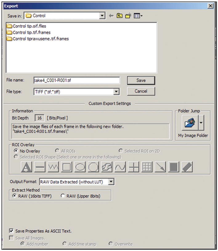
Export files window in Olympus FluoView 1.7a. This window is used to save images.

(A) RICS in cytosolic EGFP in CHO-K1 cells ● TIMING 30 min

1. With the microscope set up as described above, place the glass-bottom culture dish on the microscope stage. Incubated stages are useful for maintaining cells over long experiments but are not necessary here. The stage only needs to hold the culture dish in a stable position.

2. For image acquisition using Olympus FluoView software, click the button in the Image Acquisition Control window that turns on the mercury lamp and directs the optical path to the eyepieces (Fig. 3, circle 5).

3. Looking through the eyepieces, locate a cell and adjust the focus so that the edges of the cell are clear.

4. Once the cell is located, click the XY Repeat button (Fig. 3, circle 3) to scan the field of view continuously.

5. Set the pixel dwell time to a value between 12.5 and 20μs (Fig. 2, circle 2).

6. Most likely, no cell or only a part of a cell will appear in the scanned frame. This is because the field of view is much smaller than it appears through the eyepieces and the focus may be slightly different as well. To locate the cell, first move the ‘zoom slider’ (Fig. 2, circle 3) all the way out to increase the file of view. The LUT table may also need to be adjusted again. Thereafter, adjust the focus of the microscope to make the edges of the cell clear.

7. Zooming changes the pixel size, and zooming all the way out gives a pixel size that is too large for accurate RICS results (see INTRODUCTION). Before resetting the zoom, select a part of the cell in which to measure the diffusion coefficients and move the stage to focus on that part of the cell in the image on screen. Slowly zoom in, adjusting the stage if necessary until the region of interest (ROI) is in view at a zoom value of 16.4. Once again, this gives a pixel size of 50 nm.

8. Ensure that the cell is still in focus. Adjust the focus of the microscope as necessary. Stop the XY repeat scan by clicking the Stop button that appears below the ‘XY Repeat’ button in the Image Acquisition Control window.

   ? TROUBLESHOOTING

9. Click the ‘Time’ button that appears below the ‘Stop’ button to activate the time series scan. The ‘XYT’ button will appear. Click ‘XYT’ (Fig. 3, circle 4) to begin acquiring a series of images. It may be helpful to observe the images as they are collected to see if the cell goes out of focus or moves a great deal. The images can also be inspected after they have been collected in either Olympus FluoView or SimFCS.

10. When the scan is complete, click the ‘Series Done’ button that appears below the ‘XYT Scan’ button.

11. Save the data as described in Step 16 for analysis in Step 40A.

    ■ PAUSE POINT Analysis can be performed independently at a later time than data acquisition.

(B) RICS in EGFP–paxillin CHO-K1 cells ● TIMING 30 min

1. Repeat Step 17A(i–v) with the EGFP–paxillin CHO-K1 cells.

2. Set the pixel dwell time to a value between 12.5 and 32 μs (Fig. 2, circle 2).

3. Select a region of the cell that seems to have a focal adhesion. Focal adhesions have high concentrations of paxillin and therefore have high fluorescence intensities.

4. Return the zoom value to 16.4 (corresponding to a pixel size of 50 nm) while keeping the focal adhesion in the image.

5. Acquire and save images as described in Step 17A(viii–xi).

   ■ PAUSE POINT Analysis can be performed independently at a later time than data acquisition.

Analysis of calibration data ● TIMING 15 min

• 18Open SimFCS to calculate the beam waist on the basis of the known diffusion coefficient of EGFP.
• 19Click the ‘RICS’ button on the startup screen.
• 20Open the files associated with one RICS measurement by selecting File→ ‘Open Multiple Images (int., tif.)’.
• 21Use the file filter in the standard Windows Open File Window to view only .tif files.
• 22Select all the .tif files in the series (this should be all the files in the folder) of images saved in Step 16 and click ‘Open’. A new window will open with the frame size and data type selected. These should be loaded automatically from the text file associated with the .tif files. Close this window and the images should appear in sequence as they are loaded into SimFCS.
• 23Scroll through images using the arrows labeled ‘Image 1 frame’ (box 1 in Fig. 6).
• 24Look for aggregates (large bright spots) in the images. Delete images with aggregates using the ‘Delete frame’ button (box 2 in Fig. 6).

  ▴ CRITICAL STEP This does not delete the images from the file; it only deletes them from SimFCS.

• 25Select the frames to be processed (all of them) by setting the ‘Image 1 frame’ box to a value of 1 (box 1 in Fig. 6).
• 26Set the ‘Frames to process’ box to the number of frames acquired minus any deleted frames (box 3 in Fig. 6).
• 27Calculate image autocorrelation by selecting Tools→RICS→Subtract average (box 4 in Fig. 6). Here we use background subtraction to remove artifacts from the illumination profile. After several seconds of processing, the image correlation results should be displayed in the lower left frame.
• 28Prepare to fit the data to equation 2. From the top of the screen, select the Fit menu (box 5 in Fig. 6). The fitting window will open (Fig. 7). Note that in the displayed fitting window a fit has already been computed.
• 29
  Enter the fixed parameters for the fitting equation. Fill in the ‘Pixel time’ and ‘Line time’ boxes (box 1 in Fig. 7) with the correct times. Pixel time can be found in the text file associated with the .tif files being analyzed. Line time is not included in the .txt file. It is displayed in the Image Acquisition Settings window in Olympus FluoView as described in Step 8. If the line time was not recorded in Step 8, it can be determined by entering the same settings for zoom, objective, pixel dwell time and frame size in Olympus FluoView. Line time can also be estimated from the pixel dwell time and the length of a line, and by assuming a travel time of 4 μs per pixel on the return trip (see equation 5). This estimate is only valid for images 256 pixels wide. The ‘Frame time’ box can be ignored because RICS does not compare between frames.

  $$\text{line}\text{time}=\text{pixels}\text{per}\text{line}\times (\text{pixel}\text{dwell}\text{time}+4\mu \text{s})$$ (5)
• 30Set the ‘Pixel size’ box to 0.05 (the default units in SimFCS are μm) as determined in Step 8 and check the box next to it to fix this value in the fitting algorithm (box 2 in Fig. 7).
• 31Set the ‘Wo’ box to 0.01. ‘Wo’ is the software’s way of writing ‘ω₀’. This value is a starting guess for the fitting algorithm. Leave the box next to it unchecked so that this value can vary (box 2 in Fig. 7).
• 32Set the ‘Background’ value to 0.001 and do not fix (i.e., leave the box unchecked) (box 2 in Fig. 7).
• 33Set the ‘G1(0)’ value and leave the box unchecked (box 2 in Fig. 7). Again, this is a guess to start the fitting algorithm. A good estimate and start value of G1 is the amplitude of the correlation function that can be found in the RICS window of SimFCS (Fig. 6).
• 34Set the ‘D1’ box to 90.0 and check the box next to it (box 2 in Fig. 7). The D1 value is the known value of the EGFP diffusion coefficient³¹.
• 35Fit all the image correlations calculated. Ensure that the ‘Fit all surface’ radio button is selected. This should be the default when the program is opened (box 3 in Fig. 7).
• 36The other fields, check boxes and menus can be ignored. Most of them are used for fitting the results of other analysis techniques such as spatial temporal image correlation spectroscopy (STICS). There is one box that might be used in RICS analysis, the ‘2-photon PSF’ radio button. This should be checked when data are acquired using a two-photon laser. The use of two-photon lasers for RICS is not described here.
• 37Click the ‘Perform fit’ button (box 4 in Fig. 7). It may take several seconds, depending on the speed of your computer, to perform the fit. The computer we used had a 3.00-GHz processor and the fitting took less than a second.
• 38Display a plot of the fitting results. Select an option from the pull-down menu in the upper right (box 5 in Fig. 7). This will set the plotting options for fit. The results of the fit will always be plotted as a surface, with the x and y range the same as that of the spatial correlation. This menu selects the second plot that will also be included: the original data, the difference between the fitted surface and the data, the residuals of the fit or the fitted surface again.
• 39The results of the fit are displayed in the text at the bottom of the window (box 6 in Fig. 7). Note the calculated value for Wo. It should be between 0.2 and 0.4 μm. This value will be used to interpret data from the RICS experiments.

Figure 6.

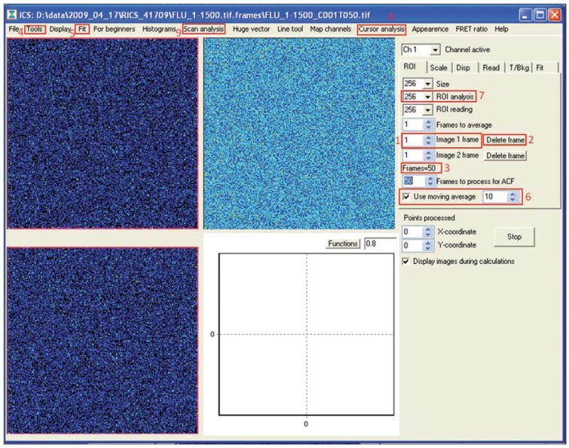
SimFCS RICS analysis screen. An image of EGFP in solution is displayed before the image correlation has been calculated. This is the primary window for RICS analysis. Box 1 contains a field that identifies the frame being displayed by number. Box 1 can be used to scroll through the images. Box 2 identifies a button that can be used to delete frames. Box 3 contains a field that can be used to select the number of frames used to calculate the autocorrelation function (auf). Box 4 contains the ‘Tools’ menu. RICS analysis options can be found under the ‘Tools’ menu. Box 5 contains the ‘Fit’ button that opens a new window with fitting options (Fig. 7). Box 6 contains a check box to select moving average subtraction and a field to choose the size of the moving average window. Box 7 contains a field that can be used to select the size of the ROI. Box 8 contains the ‘Cursor analysis’ menu. Box 9 contains the ‘Scan analysis’ menu.

Figure 7.

SimFCS fitting window. In this window the user can set the parameters required to perform a data fit. Box 1 contains fields to input the pixel dwell time and line time. Box 2 contains fields to input starting value for various fitting parameters. The check boxes next to each field can be used to determine whether the parameter will vary or be fixed. Box 3 contains a radio button that selects the ‘Fit all surface’ option. When this is selected, all the autocorrelation surfaces are used in the fitting routine. Box 4 contains the button that starts the fitting routine. Box 5 contains a drop-down menu that controls the plotted results. Box 6 contains the fitting results. Note that this view of the fitting window takes place after a fit has been calculated.

Analysis of experimental data

• 40Data analysis can be performed using Option A (for measurements in EGFP CHO-K1 cells) or Option B (for EGFP-paxillin CHO-K1 cells).

(A) Data analysis for measurements in EGFP CHO-K1 cells ● TIMING 30 min

1. Load the data from Step 17A(xi) into the RICS analysis window of SimFCS, as described in Steps 19–22.

2. Scroll through the images using the ‘Image 1 frame’ arrows (box 1 in Fig. 6). Ensure that the cell stays in focus and does not move more than can be accounted for using background subtraction according to equation 4. As a rule of thumb, discard data when the cell moves more than 1 pixel in every 5–10 frames. Background subtraction can take care of some cell motion but not if the cell moves completely out of the field of view. Frames can be deleted using the ‘Delete frame’ button (box 2 in Fig. 6). Frames with moving cellular debris moves should also be removed.

3. Select the number of frames for moving average subtraction (box 6 in Fig. 6) as described in the Experimental design section. Ten frames is an appropriate number for this experiment.

4. Perform image correlation by selecting Tool→RICS→Subtract moving average (box 4 in Fig. 6).

   ? TROUBLESHOOTING

5. Open the fitting window by selecting Fit (box 5 in Fig. 6).

6. Enter the values for pixel time and line time as described in Step 29.

7. Enter the value for pixel size (0.05) and check the adjacent box to fix this value (box 2 in Fig. 7).

8. Enter the value for ω₀ calculated in Step 39 in the box labeled ‘Wo’ and check the adjacent box to fix this value (box 2 in Fig. 7).

9. Uncheck the boxes next to ‘Background’, ‘G1(0)’ and ‘D1’ (box 2 in Fig. 7). These values are unknown and should be allowed to vary in the fitting processes.

10. Click ‘Perform fit’ (box 4 in Fig. 7).

11. The new value in the D1 box is the calculated average diffusion coefficient in the cell. However, it may be more interesting to see the range of diffusion coefficients in different regions in the cell; first close the Fit window.

12. Select an ROI analysis size from the drop-down menu (box 7 in Fig. 6). A reasonable starting value is 64 pixels.

13. Select the ‘Cursor analysis’ menu (box 8 in Fig. 6) and select ‘Toggle cursor analysis’. A pink box will appear on the image of the cell in the upper left corner of the screen (Fig. 8). The pink box defines the selected region of the cell. In it are an arrow that indicates that cursor analysis is turned on and values for G1(0) and D1 calculated with the same fitting parameters as were set in the Fit window. The plot in the lower left corner is the correlation of the selected region. The pink box can be selected with the mouse and moved around the image to find the values of G1(0) and D1 at different locations. The box must be moved slowly or there may be an error.

14. Create a map of D1 and G1(0) by selecting the ‘Scan analysis’ menu (box 9 in Fig. 6). Select ‘Scan image’, then ‘Spatial correlation.’ Save the resulting file when prompted to do so.

15. View the fit parameters by selecting the ‘Scan analysis’ menu (box 9 in Fig. 6) again and selecting ‘edit fit table’. Change the displayed parameter by adjusting the scroll bar in the ‘pfitform’ window (box 1 in Fig. 9). If any of the fit parameters appear to be outliers, it can be eliminated by changing the value to zero. Save changed parameters by selecting ‘Save modifications’ (box 2 in Figure 9). Close the pfitform window.

16. Display maps of D1 and G1(0) by selecting the ‘Scan analysis menu’ (box 9 in Fig. 6) and selecting ‘G(0) and D tables.’ A new window will open displaying intensity maps of D1 and G1(0) values. The slider under each image can be used to display both the fit parameters and the original image at the same time. The ANTICIPATED RESULTS section contains an example.

Figure 8.

Cursor analysis in the SimFCS RICS. Analysis Screen Cursor analysis rapidly displays the D and G1(0) for a user-selected ROI. Box 1 contains the raw data; the pink box within it contains the ROI and the corresponding fit values. Box 2 contains the autocorrelation, with background subtracted, for the region selected in Box 1.

Figure 9.

SimFCS pfitform Window. This window is used to edit fit parameters to create maps of D1 and G1(0). Box 1 contains arrows that can be used to scroll between fit parameters. The parameter displayed in the figure, ‘Bkgd’, is the background. Box 2 contains the ‘Save’ button.

(B) Data analysis for EGFP-paxillin CHO-K1 cells ● TIMING 30 min

1. Repeat the analysis process described in Step 40A(i–xvi) for cytosolic EGFP CHO-K1 cells.

   ▴ CRITICAL STEP The analysis procedure is the same; however, the results are expected to be different. EGFP-paxillin is interesting to study with RICS because its diffusion coefficient is different at focal adhesions than in other locations in the cell. To observe this with cursor analysis, set the ROI to 64 (box 7 in Fig. 6) at Step 40A(xii). Select the ‘Cursor analysis’ menu (box 8 in Fig. 6) and select ‘Toggle cursor analysis’ at Step 40A(xiii). Use the Cursor analysis box to identify different diffusion coefficients and concentrations of paxillin at focal adhesions and at other points in the cell. Repeat Step 40A(xiii–xvi) to create maps of G1(0) and D1 values. At focal adhesions, the diffusion coefficients should be lower and G1(0) should be higher than at other locations in the cell.

? TROUBLESHOOTING

Troubleshooting advice can be found in Table 4.

TABLE 4.

Troubleshooting table.

Step	Problem	Possible reason	Solution
12	When measuring calibration, no image can be seen even after adjusting the LUT	EGFP in solution can be difficult to distinguish from noise	One sign that the EGFP is in the focal volume and the concentration is high enough to observe is the presence of occasional aggregates—larger, brighter spots in the image. Watch for these spots before increasing the concentration of EGFP or increasing the laser power
14	Scanning does not stop after the set number of frames	The microscope may be in continuous scan mode	The ‘Time’ button (Fig. 3, circle 4) must be clicked before the ‘XYT’ button. Do not click the ‘XYRepeat’ button to save data
17A(viii)	The cell moves out of focus before RICS measurements can be made	The cell may be responding to the increased temperature from the laser	This can sometimes be solved by waiting a few minutes and letting the cell adjust to the temperature at the laser focus. Alternately, some cell movement can be accounted for by deleting frames or by subtracting background during the analysis
40A(iv)	Correlation has a diamond shape or other unusual appearance (Fig. 10)	This may be due to correlation from the shape of the cell	Make sure to select ‘RICS’ ‘subtract moving average’ from the ‘Tools’ menu. Using ‘subtract average’ will not remove all signal from the shape of the cell; this can cause strange correlation shapes. The problem may also be an inappropriate number of frames to average for moving average subtraction (box 6 in Fig. 6). See Experimental design. If neither of these solutions solves the problem, it is possible that the images have been loaded incorrectly. Close SimFCS (the entire program, not just the ‘RICS Analysis’ window) and restart

● TIMING

Defrosting and culturing of cells: 1 week (REAGENT SETUP)

Plating onto glass-bottom dishes: 1 d (REAGENT SETUP)

Steps 1–3, Setup: 30 min

Steps 4–16, Calibration of focal volume waist (ω₀) using EGFP: 15 min

Step 17A or 17B, Acquiring RICS measurements in a cell expressing a fluorescent protein: 30 min

Steps 18–39, Analysis of calibration data: 15 min

Step 40A or 40B, Analysis of experimental data: 30 min

The calibration and measurements described here can be performed in approximately 2 h.

ANTICIPATED RESULTS

The following results were obtained using the procedure described above. The images were all generated using SimFCS. Images, plots of autocorrelation and plots of fit are all displayed in false color, where intensity or magnitude corresponds to color.

Figure 10 shows an example of erroneous RICS results obtained when RICS is performed without background subtraction or with background subtraction of too few or too many frames. Figure 11a is an image of EGFP in solution. Figure 11b is the autocorrelation of EGFP in solution. The fit and difference between the fit and autocorrelation for this autocorrelation are shown in Figure 11c. This measurement is used to calibrate the beam waste. The value for ω₀ calculated here was 0.32 μm. Values can range from 0.2 to 0.4 μm.

Figure 10.

Erroneous RICS results. When RICS is performed without background subtraction or with background subtraction of too few or too many frames, the autocorrelation may have a diamond shape, as shown in this example.

Figure 11.

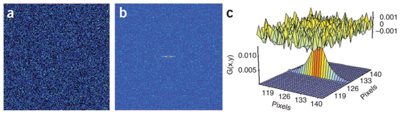
Typical results for RICS calibration measurement of EGFP in solution. (a) Raw data: the first image in the stack of images to be analyzed as displayed in SimFCS. The image is shown in false color, where color corresponds to intensity. Each image is 256 pixels by 256 pixels (12.8 μm by 12.8 μm). (b) Image correlation: the correlation peak is extended in the horizontal direction because the image is raster scanned in the horizontal direction. The horizontal axis is the horizontal correlation shift, ξ. The vertical axis is the vertical correlation shift, ψ. The color corresponds to the magnitude of the function. The correlation function is half the size of the original image, 64 pixels by 64 pixels. (c) Fit and difference: successful data fitting will result in low values for the difference between the autocorrelation and the fit. The plot at the top of the figure, the difference, should appear close to random noise. In the bottom of the figure is the result of the fit plotted in three dimensions. The height of the plot corresponds to the magnitude of the function. In both figures, the horizontal axis is the horizontal correlation shift, ξ. The vertical axis is the vertical correlation shift, ψ. The correlation fit is the same size as the original correlation function, 64 pixels by 64 pixels.

Figure 12a is an image of cytosolic EGFP in a CHO-K1 cell. The pink box is the selected ROI. Figure 12b is the autocorrelation of the region selected in Figure 12a. Note that the autocorrelation peak is wider relative to the width of the entire calculated correlation (64 pixels) in the horizontal direction than that in Figure 11b. This is because EGFP diffuses more slowly in the cell than in solution. The fit and difference between the fit and the autocorrelation are shown in Figure 12c. The diffusion coefficient for cytosolic EGFP ranges from 20 to 50 μm² s⁻¹.

Figure 12.

RICS analysis of cytosolic EGFP in a CHO-K1 cell. (a) Raw data: the first image in the stack of images to be analyzed, as displayed in SimFCS. The image is shown in false color, where color corresponds to intensity. EGFP is distributed throughout the cell. Each image is 256 pixels by 256 pixels (12.8 μm by 12.8 μm). (b) Image correlation: the correlation peak is wider in the horizontal direction than in Figure 11b because the diffusion rate is slower. The horizontal axis is the horizontal correlation shift, ξ. The vertical axis is the vertical correlation shift, ψ. The color corresponds to the magnitude of the function. The correlation function is half the size of the original image, 64 pixels by 64 pixels. (c) Fit and difference: the diffusion rate will range from 20 to 50 μm² s⁻¹. The plot at the top of the figure, the difference, should appear close to random noise. At the bottom of the figure is the result of the fit plotted in three dimensions. The height of the plot corresponds to the magnitude of the function. In both figures, the horizontal axis is the horizontal correlation shift, ξ. The vertical axis is the vertical correlation shift, ψ. The correlation fit is the same size as the original correlation function, 64 pixels by 64 pixels.

Figure 13 shows typical RICS results for EGFP-paxillin in CHO-K1 cells. It is an image of a CHO-K1 cell expressing EGFP-paxillin. Note that in contrast to cytosolic EGFP, EGFP-paxillin is not distributed evenly throughout the cell. Paxillin is more concentrated at focal adhesions. In this image, the pink box selects the ROI analysis. Figure 13b is the autocorrelation of the ROI analysis selected in Figure 13a. The fit and difference between the fit and autocorrelation are shown in Figure 13c. Diffusion coefficients for EGFP-paxillin range from 1 to 20 μm² s⁻¹.

Figure 13.

RICS analysis of EGFP-paxillin in a CHO-K1 cell. (a) Raw data: the first image in the stack of images to be analyzed as displayed in SimFCS. The image is shown in false color, in which color corresponds to intensity. EGFP-paxillin is seen at higher concentrations near focal adhesions. Each image is 256 pixels by 256 pixels (12.8 μm by 12.8 μm). (b) Image correlation: image correlation is calculated at the region of interest selected with the pink box in a. The horizontal axis is the horizontal correlation shift, ξ. The vertical axis is the vertical correlation shift, ψ. The color corresponds to the magnitude of the function. The correlation function is half the size of the original image, 64 pixels by 64 pixels. (c) Fit and difference: the diffusion rate will range from 1 to 20 μm² s⁻¹. The plot at the top of the figure, the difference, should appear close to random noise. At the bottom of the figure is the result of the fit plotted in three dimensions. The height of the plot corresponds to the magnitude of the function. In both figures, the horizontal axis is the horizontal correlation shift, ξ. The vertical axis is the vertical correlation shift, ψ. The correlation fit is the same size as the original correlation function, 64 pixels by 64 pixels.

References

- 1.Digman MA, et al. Measuring fast dynamics in solutions and cells with a laser scanning microscope. Biophys J. 2005;89:1317–1327. doi: 10.1529/biophysj.105.062836. [DOI] [PMC free article] [PubMed] [Google Scholar]
- 2.Digman MA, et al. Fluctuation correlation spectroscopy with a laser-scanning microscope: exploiting the hidden time structure. Biophys J. 2005;88:L33–L36. doi: 10.1529/biophysj.105.061788. [DOI] [PMC free article] [PubMed] [Google Scholar]
- 3.Pawley JB. Handbook of Biological Confocal Microscopy. 3. Springer; New York, USA: 2006. [Google Scholar]
- 4.Webb RH. Confocal optical microscopy. Rep Prog Phys. 1996;59:427–471. [Google Scholar]
- 5.Wiseman PW, Squier JA, Ellisman MH, Wilson KR. Two-photon image correlation spectroscopy and image cross-correlation spectroscopy. J Microsc. 2000;200:14–25. doi: 10.1046/j.1365-2818.2000.00736.x. [DOI] [PubMed] [Google Scholar]
- 6.Wiseman PW, et al. Spatial mapping of integrin interactions and dynamics during cell migration by image correlation microscopy. J Cell Sci. 2004;117 (Part 23):5521–5534. doi: 10.1242/jcs.01416. [DOI] [PubMed] [Google Scholar]
- 7.Petersen NO, Höddelius PL, Wiseman PW, Seger O, Magnusson KE. Quantitation of membrane receptor distributions by image correlation spectroscopy: concept and application. Biophys J. 1993;65:1135–1146. doi: 10.1016/S0006-3495(93)81173-1. [DOI] [PMC free article] [PubMed] [Google Scholar]
- 8.Digman MA, Gratton E. Analysis of diffusion and binding in cells using the RICS approach. Microsc Res Tech. 2009;72:323–332. doi: 10.1002/jemt.20655. [DOI] [PMC free article] [PubMed] [Google Scholar]
- 9.Bihan DL. Molecular diffusion, tissue microdynamics and microstructure. NMR Biomed. 1995;8:375–386. doi: 10.1002/nbm.1940080711. [DOI] [PubMed] [Google Scholar]
- 10.Weaver JL, Prestegard JH. Nuclear magnetic resonance structural and ligand binding studies of BLBC, a two-domain fragment of barley lectin. Biochemistry. 1998;37:116–128. doi: 10.1021/bi971619p. [DOI] [PubMed] [Google Scholar]
- 11.Birge RB, et al. Identification and characterization of a high-affinity interaction between v-Crk and tyrosine-phosphorylated paxillin in CT10-transformed fibroblasts. Mol Cell Biol. 1993;13:4648–4656. doi: 10.1128/mcb.13.8.4648. [DOI] [PMC free article] [PubMed] [Google Scholar]
- 12.Harlow E, Whyte P, Franza BR, Jr, Schley C. Association of adenovirus early-region 1A proteins with cellular polypeptides. Mol Cell Biol. 1986;6:1579–1589. doi: 10.1128/mcb.6.5.1579. [DOI] [PMC free article] [PubMed] [Google Scholar]
- 13.Clegg RM. In: Fluorescence Imaging Spectroscopy and Microscopy. Wang XF, Herman B, editors. Vol. 137. Wiley; 1996. pp. 179–251. [Google Scholar]
- 14.Kreis TE, Geiger B, Schlessinger J. Mobility of microinjected rhodamine actin within living chicken gizzard cells determined by fluorescence photobleaching recovery. Cell. 1982;29:835–845. doi: 10.1016/0092-8674(82)90445-7. [DOI] [PubMed] [Google Scholar]
- 15.Scherson T, et al. Dynamic interactions of fluorescently labeled microtubule-associated proteins in living cells. J Cell Biol. 1984;99:425–434. doi: 10.1083/jcb.99.2.425. [DOI] [PMC free article] [PubMed] [Google Scholar]
- 16.Elson EL, Madge D. Fluorescence correlation spectroscopy: I. Conceptual basis and theory. Biopolymers. 1974;13:1–27. doi: 10.1002/bip.1974.360130103. [DOI] [PubMed] [Google Scholar]
- 17.Kim SA, Heinze KG, Bacia K, Waxham MN, Schwille P. Two-photon cross-correlation analysis of intracellular reactions with variable stoichiometry. Biophys J. 2005;88:4319–4336. doi: 10.1529/biophysj.104.055319. [DOI] [PMC free article] [PubMed] [Google Scholar]
- 18.Wiseman PW, Petersen NO. Image correlation spectroscopy. II. Optimization for ultrasensitive detection of preexisting platelet-derived growth factor-[beta] receptor oligomers on intact cells. Biophys J. 1999;76:963–977. doi: 10.1016/S0006-3495(99)77260-7. [DOI] [PMC free article] [PubMed] [Google Scholar]
- 19.Kolin DL, Wiseman PW. Advances in image correlation spectroscopy: measuring number densities, aggregation states, and dynamics of fluorescently labeled macromolecules in cells. Cell Biochem Biophys. 2007;49:141–164. doi: 10.1007/s12013-007-9000-5. [DOI] [PubMed] [Google Scholar]
- 20.Vendelin M, Birkedal R. Anisotropic diffusion of fluorescently labeled ATP in rat cardiomyocytes determined by raster image correlation spectroscopy. Am J Physiol Cell Physiol. 2008;295:C1302–C1315. doi: 10.1152/ajpcell.00313.2008. [DOI] [PMC free article] [PubMed] [Google Scholar]
- 21.Gielen E, et al. Measuring diffusion of lipid-like probes in artificial and natural membranes by raster image correlation spectroscopy (RICS): use of a commercial laser-scanning microscope with analog detection. Langmuir. 2009;25:5209–5218. doi: 10.1021/la8040538. [DOI] [PMC free article] [PubMed] [Google Scholar]
- 22.Watson NB, et al. RAD18 and associated proteins are immobilized in nuclear foci in human cells entering S-phase with ultraviolet light-induced damage. Mutat Res. 2008;648:23–31. doi: 10.1016/j.mrfmmm.2008.09.006. [DOI] [PMC free article] [PubMed] [Google Scholar]
- 23.Sanabria H, Digman MA, Gratton E, Waxham MN. Spatial diffusivity and availability of intracellular calmodulin. Biophys J. 2008;95:6002–6015. doi: 10.1529/biophysj.108.138974. [DOI] [PMC free article] [PubMed] [Google Scholar]
- 24.Digman MA, Wiseman PW, Horwitz AR, Gratton E. Detecting protein complexes in living cells from laser scanning confocal image sequences by the cross correlation raster image spectroscopy method. Biophys J. 2009;96:707–716. doi: 10.1016/j.bpj.2008.09.051. [DOI] [PMC free article] [PubMed] [Google Scholar]
- 25.Frigault MM, Lacoste J, Swift JL, Brown CM. Live-cell microscopy—tips and tools. J Cell Sci. 2009;122 (Part 6):753–767. doi: 10.1242/jcs.033837. [DOI] [PubMed] [Google Scholar]
- 26.Brown CM. Fluorescence microscopy—avoiding the pitfalls. J Cell Sci. 2007;120 (Part 10):1703–1705. doi: 10.1242/jcs.03433. [DOI] [PubMed] [Google Scholar]
- 27.Brown CM, et al. Raster image correlation spectroscopy (RICS) for measuring fast protein dynamics and concentrations with a commercial laser scanning confocal microscope. J Microsc. 2008;229:78–91. doi: 10.1111/j.1365-2818.2007.01871.x. [DOI] [PMC free article] [PubMed] [Google Scholar]
- 28.Digman MA, Brown CM, Horwitz AR, Mantulin WW, Gratton E. Paxillin dynamics measured during adhesion assembly and disassembly by correlation spectroscopy. Biophys J. 2008;94:2819–2831. doi: 10.1529/biophysj.107.104984. [DOI] [PMC free article] [PubMed] [Google Scholar]
- 29.Phela MC. In: Current Protocols in Cell Biology. Bonifacino JS, et al., editors. Vol. 1. Wiley; 1998. pp. 1.1.1–1.1.18. Ch. 1. [Google Scholar]
- 30.Chishima T, et al. Metastatic patterns of lung cancer visualized live and in process by green fluorescence protein expression. Clin Exp Metastasis. 1997;15:547–552. doi: 10.1023/a:1018431128179. [DOI] [PubMed] [Google Scholar]
- 31.Potma EO, et al. Reduced protein diffusion rate by cytoskeleton in vegetative and polarized dictyostelium cells. Biophys J. 2001;81:2010–2019. doi: 10.1016/s0006-3495(01)75851-1. [DOI] [PMC free article] [PubMed] [Google Scholar]