Application of a Rat Hindlimb Model: A Prediction of Force Spaces Reachable Through Stimulation of Nerve Fascicles

Abstract

A device to generate standing or locomotion through chronically placed electrodes has not been fully developed due in part to limitations of clinical experimentation and the high number of muscle activation inputs of the leg. We investigated the feasibility of functional electrical stimulation paradigms that minimize the input dimensions for controlling the limbs by stimulating at nerve fascicles, utilizing a model of the rat hindlimb which combined previously collected morphological data with muscle physiological parameters presented herein. As validation of the model we investigated the suitability of a lumped-parameter model for prediction of muscle activation during dynamic tasks. Using the validated model we found that the space of forces producible through activation of muscle groups sharing common nerve fascicles was nonlinearly dependent on the number of discrete muscle groups that could be individually activated (equivalently, the neuroanatomical level of activation). Seven commonly innervated muscle groups were sufficient to produce 78% of the force space producible through individual activation of the 42 modeled hindlimb muscles. This novel, neuroanatomically derived reduction in input dimension emphasizes the potential to simplify controllers for functional electrical stimulation to improve functional recovery after a neuromuscular injury.

I. Introduction

Functional electrical stimulation (FES) devices are used to restore motor function after impairment in the central nervous system. For example, there currently exist devices to assist standing and to reduce foot drop [1]–[3] in individuals with a neural impairment. However, a device to generate locomotion with chronically placed electrodes has not been fully developed because of several complicating factors. Human studies are complicated by variations in injuries, ethical considerations, and cost. Consequently animal models, and the rat in particular, are widely used for the development and evaluation of rehabilitative treatment strategies [4]–[6]. A second complicating factor in FES development is that the number of muscles to be controlled is large. For instance, in the case of the human leg there are five degrees of freedom corresponding to the joints and approximately forty inputs corresponding to the muscles, many of which are redundant actuators. A controller of such a high-dimensional system could suffer from high computational cost. Therefore, reducing the number of inputs by stimulating groups of muscles at their common nerve would be desirable. Stimulating motor nerves can also be desirable for achieving more natural patterns of muscle fiber recruitment and potentially reducing muscle fatigue [7],[8].

Here we use a rat model to show that nerve-based FES strategies can reduce the number of input dimensions needed to control the limbs. Specifically, we tested the hypothesis that constraining muscles to activate in commonly innervated groups, as would be the case with FES at nerve fascicles, does not substantially compromise the ability of the limb to produce forces appropriate for locomotion.

The definition of commonly innervated, i.e., neuroanatomically derived, muscle groups parallels current work investigating the simplifying effects of muscle synergies on the neural control of movement [9]–[11]. Muscle synergies mediate motor task planning and execution, acting as an abstraction layer to produce specific muscle activation patterns given goal-based kinetic or kinematic demands. Muscle synergies could effectively reduce the dimensions of the musculoskeletal system that must be controlled by the nervous system. Similarly, neuroanatomically derived muscle grouping could simplify FES by reducing the variables that must be controlled by an artificial controller.

To investigate the suitability of neuroanatomically derived groups for producing standing and locomotion we have evaluated force production associated with stimulation of nerve fascicles. To calculate the effects of individual muscle forces a model of the musculoskeletal system of the hindlimb is required. Previous studies have characterized the musculoskeletal morphology, segmental mechanics, and activation dynamics necessary for a dynamic musculoskeletal model [12]–[14]. In addition to these parameters, models of contraction dynamics must be chosen. We chose a lumped-parameter formulation [13],[14] that adequately represents force production of the muscle while remaining computationally efficient enough to allow modeling of the complete hindlimb. As an extension of model validation, we compared model predicted muscle activation to measured EMG during a dynamic task, i.e., locomotion. The close agreement between model predicted and measured activations lends support to the use of lumped-parameter musculoskeletal models for simulation of gait dynamics.

The purpose of the present study was to determine the effects of constraining muscle activation to neuroanatomically derived groups on the space of forces producible by the hindlimb. We studied four postures associated with locomotion. The space of forces producible through idealized excitation of different groupings of neuroanatomically-derived muscles was determined and compared among postures. We also quantitatively compared the sizes of the producible force spaces associated with varying numbers of muscle groups. We found that activation of the muscles of as few as 7 nerve fascicles was required to approximately reproduce the natural force space of the hindlimb during locomotion.

II. Methods

A. Muscle Physiology

Ethical approval

All procedures were approved by the UCLA Chancellor’s Animal Research Committee and followed the American Physiological Society Animal Care Guidelines.

Muscle measurements

Muscle physiological parameters were taken from rats of similar size, age, and sex as those used previously to define the morphology of the limb [12], and normalized to a rat body mass of 300 g. These data were used as parameter values for a lumped-parameter model of muscle [15] with the following muscle-specific parameters: maximum isometric force (P₀), maximum shortening velocity (v_max), optimal fiber length (l₀), pennation angle at optimal length (θ₀), and tendon slack length (l_ts).

Muscle architectural measurements

Four rats of matching mass (294 ± 7 g) were used for muscle architectural measurements as described previously [15]. The rats were perfused intracardially with 8% paraformaldehyde with the ankle, knee, and hip joints fixed at ~90°, then the isolated and skinned hindquarters immersed in 4% paraformaldehyde for three days. Individual muscles were dissected and submerged in 20% sulfuric acid solution to soften connective tissue, then stored in phosphate buffer solution until measurement. Whole muscle length (l′_m) excluding the tendon was measured along the muscle line of action. Fiber pennation angle (θ′) was measured relative to the line of action. Muscles with multiple compartments were divided and the angle of pennation measured for each compartment. Small muscle fascicles (10 to 20 fibers) were teased from several regions of the muscle and their lengths (l′) measured. Individual fibers were teased from the fascicles and mounted on slides. Sarcomere length (l′s) was measured under high magnification in three locations on each fiber and averaged to account for non-uniform sarcomere lengths. Because all measurements were taken at generally sub-optimal muscle length, corrections were calculated to produce optimal fiber length and pennation angle. Optimal fiber length was calculated from the measured fiber length and sarcomere length as

$$l_0=l^{\prime }·\frac{l_{0s}}{l_s^{\prime }}$$

where l_0s = 2.40 μm (see Discussion) is the optimal sarcomere length taken from the literature [15]–[17] and assumed to be constant across all muscles. Pennation angle at optimal fiber length was likewise corrected for the geometric effect of the sub-optimal length as

$${\theta }_0=arcsin\left(\frac{l^{\prime }sin{\theta }^{\prime }}{l_0}\right).$$

Maximum isometric force and maximum contraction velocity were calculated as

$$P_0=\frac{mcos{\theta }_0}{l_0\rho }·T{v}_{max}=v_s·\frac{l_0}{l_{0s}}$$

where ρ = 1.056 g cm⁻³ is muscle density and T = {15.70, 22.94} g mm⁻² and v_s= {13.4, 42.7} μm s⁻¹, are specific tension and sarcomere shortening velocities for slow and fast fibers, respectively. Muscle specific tensions and sarcomere shortening velocities were assumed to be constant within fiber type [15],[18]. Furthermore, sarcomere shortening was assumed to be homogeneous along the fiber length and fiber lengths were averaged across the muscle breadth, as is consistent with the established lumped-parameter model [13], [14],[19]. The architecture experiment produced all muscle-specific parameters defining muscle force generation, i.e., P₀, v_max, θ₀, and l₀.

Muscle electrophysiology measurements

Only fourteen muscles allowed direct physiological experiments to be performed due to limitations in isolating the insertion of proximal muscles, particularly those with broad or multipennate structure such as GMa. Electrophysiological measurements were therefore taken not for model definition, but for validation of the architectural measurement method used to define the model muscle parameters. The mechanical properties of each muscle were determined in situ in two rats. Up to two muscles could be measured in any one rat, and six rats yielded data from only one muscle, resulting in a total of 17 rats (276 ± 15 g). Measurements were taken in the manner described by Roy et al. [20]. The rat was anesthetized deeply (100 mg kg⁻¹ ketamine plus 5 mg kg⁻¹ xylazine, i.p., supplemented with ketamine as required), the muscle isolated, and its distal tendon cut and attached via silk ligature to a force transduction lever (Model 305B-LR; Aurora Scientific, Toronto, Ontario, Canada). Individual nerves were isolated and stimulated with bipolar silver electrodes. Stimulus voltage was twice the minimum voltage required to elicit a twitch, typically 4–6 V. Body and muscle temperatures were maintained throughout the experiment at 34–36°C. The P₀ was found by applying tetanic stimulation (0.2 ms monophasic square wave pulses at 200 Hz, train duration 300 ms) at varying muscle lengths. The muscle was stimulated with a single 0.2 ms pulse and allowed to freely contract to a self-selected short length. It then was lengthened in 1 mm increments and a tetanic stimulation applied at each length. Rest times of 2 min duration were maintained between each stimulus, during which single 0.2 ms pulses were applied every 30 s. The peak force measured during any tetanic stimulation was taken as P₀, and the length at which it occurred as the optimal muscle length l_0m.

The v_max was found via the afterload technique, i.e., applying a tetanic stimulation to the muscle at its optimal length l_0m, and allowing the muscle to contract against a submaximal isotonic load. Eight to ten contractions were elicited at loads ranging from the passive tension at l_0m to approximately one third P₀. The measured forces and velocities were fit to the Hill force-velocity equation [21] as

$$P=F_v(v)=\frac{b_1-b_{2}v}{b_1+v}$$

and the b parameters estimated using non-linear least-squares. F_v(v) was inverted and evaluated at zero load to calculate the maximum shortening velocity:

$$v_{max}={F_v^{-1}(P)\mid }_{P=0}.$$

Mass normalization

Although the musculoskeletal geometry and muscle architecture measurements were taken from rats of similar mass, i.e., within a 40 g range, additional normalization to account for mass was required. Normalization is assisted by the assumption that all components of the rat scale proportionately and that the densities are constant. Following the square-cube law, P₀ scales with the two-thirds power of mass ratio, while v_max, l₀ and l_ts scale with the cube root of mass ratio.

B. Musculoskeletal Model Validation

To validate the combined morphological and physiological parameters that define the model, we performed locomotion experiments. Twelve rats matching the sex and body mass of the rats used for the physiology experiments were implanted with intramuscular EMG electrodes and made to walk on an instrumented trackway. EMG, kinematics, and ground reaction forces were recorded. The experimental kinematics and ground reaction forces were analyzed using inverse dynamics and static optimization to estimate individual muscle activation levels. The estimated activations were compared to the experimental EMG to validate the model.

Musculoskeletal model definition

The physiological parameters presented herein were combined with morphological parameters defined previously and presented in [12]. Briefly, the hindlimb was modeled as a five degrees of freedom (DOF) linkage comprising a three-DOF hip joint and single DOF knee and ankle joints. The hip segment was fixed to a specified trajectory, and forces and torques could not alter its movement. Fixing the hip segment was necessary, as an unconstrained hip segment would require modeling the dynamics of the entire body, which was outside the scope of the present study. The foot-ground interface was modeled as a spherical joint, with reaction forces applied to the model as measured in locomotion experiments.

EMG electrode implantation

EMG electrode implant surgeries were carried out under aseptic conditions as described previously [22]. Rats were anesthetized deeply using 1–3% isoflurane gas. The dorsal aspect of the skull was exposed and dried thoroughly. Five screws were driven into the skull and two 9-pin amphenol connectors were anchored to the skull and screws with dental cement. Sixteen Teflon-coated stranded stainless steel wires were led subcutaneously from the connectors to the right hindlimb. About 1 cm of the Teflon coating was removed from the distal end of a seventeenth wire, which was embedded in the middle-back region and served as a common ground. The ST, BFa, GMa, VL, RF, TA, Sol and MG muscles were exposed (for muscle abbreviations see Table 2), and two wires were inserted into each muscle by passing them individually through a 23-gauge hypodermic needle. Recording electrodes were made by removing ~0.5–1.0 mm of insulation from each wire and positioning the electrodes in the mid-belly of the muscle. Following stimulation of the muscle through the electrode to ensure proper placement, each lead was secured with a suture at its entry and exit from the muscle. The bared tips of the wires were covered by gently pulling the Teflon coating over the tips to avoid recording extraneous potentials. Rats were allowed to recover for at least five days before locomotion testing began.

Table 2.

Muscle-specific physiology parameters taken from architectural and electrophysiological measurements as described in the Methods. Muscle masses are normalized to a rat body mass of 300 g. Architectural values were used in the musculoskeletal model. Unless otherwise indicated, architectural measurements including mass, optimal fiber length, maximum isometric tension and maximum shortening velocity were taken from n=4 rats, while electrophysiological measurements of maximum isometric tension and shortening velocity, and tendon slack lengths were taken from n=2 rats.

Abbreviation		Muscle Name	Mass (mg)	l0 (mm)	θ0 (deg)	P0 (g) Architecture	P0 (g) Physiology	vmax (mm s−1)Architecture	vmax (mm s−1) Physiology	lts (mm)
	AB	adductor brevis	1087 ±157	22.8 ±0.4	12 ± 5	1246 ±80		406 ± 21		0±0
	AL	adductor longus	94 ± 19	16.6 ±2.1	9± 4	106 ± 15		93 ± 17		4.5 ± 0.3
	AM	adductor magnus	280 ±93	28.4 ±1.0	0± 0	308 ± 24		506 ± 32		0±0
	BFa	biceps femoris anterior	470 ± 99	39.7 ± 3.9	0± 1	346 ± 23		706 ± 60		0±0
	BFp	biceps femoris posterior	1655 ± 348	37.6 ± 1.7	7± 5	1274 ± 83		669 ± 71		0±0
	CF	caudofemoralis	275 ± 91	37.9 ± 3.2	0± 0	210 ± 25		675 ± 77		0±0
	EDL	extensor digitorum longus	146 ± 14	13.7 ±1.0	10 ± 3	225 ± 8	265 ± 65	243 ± 15	205 ± 13	9.0 ± 0.4
	EHL	extensor hallucis longus	13±2	12.1 ±0.8	5± 3	25 ± 2		216 ± 22		13.6±1.2
	FDL	flexor digitorum longus	470 ± 53	9.0 ± 0.5	11 ± 5	1124 ±217	1344 ± 494	160 ± 33	140 ± 17	8.7 ± 0.8
	FHL	flexor hallucis longus	22 ± 1	10.8 ±1.0**	2± 4**	45 ± 1**		193 ± 6**		9.7 ± 0.0
	GI	gemellus inferior	55 ± 2	4.2 ± 0.2	18 ± 7	291 ± 38		74 ± 9		0±0
	GS	gemellus superior	12 ±2	6.1 ± 1.1	10 ± 14	38 ± 13		109 ± 31		0±0
	GMa	gluteus maximus	793 ± 33	19.6 ±4.7	12 ± 10	942 ± 276		349 ± 75		4.8 ± 0.4
	GMe	gluteus medius	1444 ± 182	19.9 ±2.7	12 ± 2	1912 ± 233		355 ± 35		0±0
	GMi	gluteus minimus	378 ± 25	11.8 ±0.3	16 ± 9	754 ± 61		211 ± 22		0±0
	GA	gracillis anterior	168 ± 32	30.3 ± 4.9	0± 0	158 ± 10		539 ± 50		0±0
	GP	gracillis posterior	246 ± 43	29.3 ± 4.1	3± 4	240 ± 35		163 ± 27		0.9 ± 0.1
	IP	iliacus	999 ± 77	22.3 ± 0.9*	7± 4*	1043 ± 84*		402 ± 50*
		psoas major	1179 ± 126	23.8 ± 3.3*	15 ± 3*	1151 ±157*		418 ± 64*		4.1 ± 0.0
	LG	lateral gastrocnemius	805 ± 161	12.5 ±0.8	9± 6	1863 ± 116	1734 ± 43	223 ± 17	209 ± 17	9.4 ± 0.3
	MG	medial gastrocnemius	720 ± 56	14.6 ± 0.4	13 ± 4	1188±92	1364 ± 30	260 ± 25	238 ± 6	9.1 ±0.3
	OE	obturator externus	194 ± 13	6.0 ± 0.8	16 ± 6	732 ±80		106 ± 10		0±0
	OI	obturator internus	54 ± 11	4.5 ± 0.7	7± 6	307 ± 35		81 ± 10		2.8 ± 4.0
	Pec	pectineus	233 ± 17	10.9 ±0.7*	7± 1*	503 ± 14*		193 ± 2*		0±0
Per	PerB	peroneus brevis	88 ± 11	8.6 ± 0.9	6± 7	243 ± 20	501 ± 40	152 ± 16	117±4	10.3 ± 0.2
	PerL	peroneus longus	131 ± 16	7.6 ± 0.3	9± 2	404 ± 32	622 ± 122	135 ± 12	113±7	12.7 ±0.1
	PerQa	peroneus digiti quarti	31 ± 4	8.8 ± 1.9	7± 5	86 ± 15	139 ± 2	157 ± 36	116±19	9.1 ± 1.4
	PerQi	peroneus digiti quinti	21 ± 3	8.6 ± 0.8*	4± 1*	56 ± 3*	113 ± 22	152 ± 13*	116±4	19.6 ± 0.9
	Pir	piriformis	478 ± 60	10.8±1.6	16 ± 8	1137±123		193 ± 19		0±0
	Pla	plantaris	308 ± 27	12.5±1.5	11 ± 4	572 ± 56	792 ± 13	223 ± 17	207 ± 13	6.7 ± 0.2
	Pop	popliteus	90 ± 5	6.5 ± 0.6	13 ± 6	298 ± 17		115±5		0±0
	QF	quadratus femoris	155 ± 14	11.0±1.0	3± 2	306 ± 18		197 ± 15		0±0
	SM	semimembranosus	1291 ± 320	35.7 ± 1.0	0± 0	1043 ± 69		634 ± 57		0±0
ST	STa	semitendinosus accessory	177 ± 25	34.1 ± 6.4	0± 0	142 ± 23		607 ± 95		0±0
	STp	semitendinosus principal	707 ± 101	43.6 ± 10.4	0± 0	463 ± 148		775 ± 193		0±0
	Sol	soleus	155 ± 27	16.0 ±5.1	4± 9	145 ± 27	234 ± 29	89 ± 22	93 ± 11	9.5 ± 0.5
	TFL	tensor fascia latae	362 ± 15	20.6 ± 0.6*	11 ± 8*	397 ± 30*		367 ± 27*		0±0
	TA	tibialis anterior	542 ± 60	15.2 ±0.7	9± 4	878 ± 81	1004 ± 45	271 ± 29	290 ± 6	11.9±1.5
	TP	tibialis posterior	85 ± 5	5.4 ± 1.4	5± 3	361 ± 83	605 ± 51	97 ± 31	68 ± 1	12.4 ±0.2
	RF	rectus femoris	900 ± 67	12.2 ±0.9	11 ± 5	1681 ± 86	1859 ± 71	216 ± 19	227 ± 13	6.6 ± 0.8
	VI	vastus intermedius	181 ± 12	11.6 ±0.6	14 ± 3	260 ± 25		65 ± 9		6.6 ± 0.8
	VL	vastus lateralis	1113 ± 170	19.8 ± 0.3	14 ± 3	1517 ± 79		352 ± 25		6.6 ± 0.8
	VM	vastus medialis	396 ± 26	15.6±1.3	11 ± 6	620 ± 73	611 ± 87	278 ± 34	161 ± 3	6.6 ± 0.8

^*n=3

^**n=2.

Locomotion testing methods

Rats were tested walking quadrupedally on a level trackway at a self-selected pace. Two days of testing were performed, on each of which the rats were made to walk across the trackway five times. Trials in which the rat contacted the force platform only with its right hindlimb were retained for a total of 47 trials. EMG signals were amplified, recorded and displayed using a computer data acquisition system (LabVTEW, National Instruments Inc., Austin, TX). Reflective markers were placed on the right torso (iliac crest), hip (greater trochanter), knee (lateral condyle), ankle (lateral malleolus), and foot (fourth metatarsal). Locomotion was filmed at 100 Hz using two cameras with angular offset. 3-D marker positions were tracked using stereophotogrammetry as implemented by SIMI (SIMI Reality Motion Systems GmbH, Unterschleissheim, Germany). Reaction force was measured with a commercial six-axis force platform (HE6X6, AMTI, Watertown, MA) and recorded using the LabVIEW system.

Inverse dynamics and static optimization

Model analysis was performed in the open source OpenSim musculoskeletal modeling environment [23]. Limb kinematics were calculated from 3-D marker positions using a weighted least-squares method to mitigate the effects of skin motion. Inverse dynamics was performed to find joint torques given the experimental kinematics and ground reaction forces. Muscle physiology was modeled with a lumped-parameter formulation [13],[14],[19]. Static optimization was used to distribute joint torques across the redundant muscles while minimizing muscle activation as described in [24]. The objective function in this case was

$$J(t)=\sum _{i=1}^{n}a{(t)}^4$$

where n = 39 is the number of muscles and a is muscle activation at time t. The objective function was minimized subject to the constraints that force production of individual muscles was tensile and that joint torques balanced muscle moments:

$$f_i(t)\ge 0,{\tau }_k=\sum _{j=1}^n{f}_j(t)r_{j,k}(t)$$

where f_i is the force produced by muscle i, r_j,k is the scalar moment arm of muscle j about joint k, and τ_k is the torque at joint k.

C. Force Envelopes

When activated, a hindlimb muscle produces a torque at each joint it crosses. The postural configuration of the limb determines the resultant force (magnitude and direction) produced at the foot. The magnitude of the resultant force is scaled by the activation level, which is defined as varying from zero (no activation) to one (full activation). The space of producible forces is the union of all force vectors produced by summing the resultant forces of the individual muscles in all possible combinations and at all levels of activation. The space of producible forces may be visualized as a 3-D volume about the foot. When muscles are grouped, i.e., constrained to activate at equal levels, the net force produced by the group is the sum of the force vectors produced by each muscle individually, scaled by the group activation. Therefore, if the grouped muscles were allowed to activate independently they would be capable of producing forces in a number of directions, but grouping them constrains their net force to one direction and thus reduces the space of producible forces.

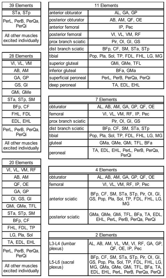
The effect of constraining the hindlimb muscles to be activated based on common innervation was investigated at four postures corresponding to four points in the gait cycle: toe off, mid-swing, toe contact, and mid-stance. The number of inputs, i.e., activations, was reduced by grouping commonly innervated muscles and by constraining all muscles within the group to have the same activation level. Muscle innervation patterns were defined according to Greene [25] and confirmed by observation during dissection (Fig. 1). Muscles were grouped with varying levels of specificity, from the trivial case in which each group consisted of one muscle (ST and Per modeled as a single muscle each) to the general case of two groups corresponding to excitation of the sacral and caudal lumbar plexuses (Table 1). For a given posture and for each level of group specificity, the space of producible forces was defined as all linear combinations with coefficients between zero and one of the force vectors generated at the ball of the foot by the muscle groups. In other words, the space of producible forces is the set of all forces that could be produced at the foot by activating the muscle groups in any combination.

Figure 1.

A map of the innervation pattern of the rat hindlimb muscles. Muscles are depicted as nodes (abbreviations found in Table 2). Nerves and nerve fascicles are depicted as branches. Labels of the branches correspond to the muscle groups used in constructing feasible force envelopes in Table and 1. Grouping are derived from Greene [25] and direct observations during dissection of the limbs.

Table 1.

Muscle groupings used to generate feasible force envelopes. The number of individually excitable elements (groups plus individual muscles not in a group) is shown above each group. If a group corresponds to excitation of a particular nerve, it is listed to the left of the group. Prox = proximal; dist = distal.

Force space projections

Extremal points (i.e., vertices) of the force space are a subset of all combinations of muscle force vectors at maximal activation. Because the number of muscle groups and thus the number of force vectors was large, it was impractical to analytically determine the space of all linear combinations of those vectors. For example, there are 2⁴²≈4.4·10¹² combinations in the individual muscle case. Instead a synthetic method was used to closely approximate the polygons associated with projection of the force space onto the anatomical planes. Bounding boxes defining the maximum extent of the force space in the directions of the axes were found as the axes were rotated; the intersection of the bounding boxes approximated the force space projection. The following formalization uses the sagittal plane as an example.

First the set of resultant force vectors at the foot (v_i, i ∈ {1, …,n}) was calculated, where n is the number of muscle groups. The space of producible vectors is

$$\mathit{V}=\left\{\left[\begin{array}{c}{v}_x\\ v_y\end{array}\right]:\left[\begin{array}{c}{v}_x\\ v_y\end{array}\right]=\sum _{i=1}^n{\alpha }_i{\mathit{v}}_i\wedge {\alpha }_i\in [0,1]\right\}.$$

Then a box (B₀) bounding V was defined as the maximum and minimum values of the combined vectors’ components,

$${\mathit{B}}_0=\left\{\left[\begin{array}{c}{v}_{x,min}\\ v_{y,min}\end{array}\right],\left[\begin{array}{c}{v}_{x,min}\\ v_{y,max}\end{array}\right],\left[\begin{array}{c}{v}_{x,max}\\ v_{y,max}\end{array}\right],\left[\begin{array}{c}{v}_{x,max}\\ v_{y,min}\end{array}\right]\right\}$$

where

$$\begin{array}{cccc}{v}_{x,min}=\sum v_x& v_x<0& v_{x,max}=\sum v_x& v_x>0\\ v_{y,min}=\sum v_y& v_y<0& v_{y,max}=\sum v_y& v_y>0\end{array}$$

The basis of the projection plane then was rotated by an arbitrary rotation matrix R,

$$\left[\begin{array}{c}{v}_x^{\prime }\\ v_y^{\prime }\end{array}\right]=\sum _{i=1}^n{\alpha }_i{\mathit{Rv}}_i$$

extremal points found in the new basis,

$$\begin{array}{cccc}{v}_{x,min}^{\prime }=\sum v_x^{\prime }& v_x^{\prime }<0& v_{x,max}^{\prime }=\sum v_x^{\prime }& v_x^{\prime }>0\\ v_{y,min}^{\prime }=\sum v_y^{\prime }& v_y^{\prime }<0& v_{y,max}^{\prime }=\sum v_y^{\prime }& v_y^{\prime }>0\end{array}$$

and the extremal points rotated back to produce a rotated bounding box (B₁).

$${\mathit{B}}_1=\left\{{\mathit{R}}^{-1}\left[\begin{array}{c}{v}_{x,min}^{\prime }\\ v_{y,min}^{\prime }\end{array}\right],{\mathit{R}}^{-1}\left[\begin{array}{c}{v}_{x,min}^{\prime }\\ v_{y,max}^{\prime }\end{array}\right],{\mathit{R}}^{-1}\left[\begin{array}{c}{v}_{x,max}^{\prime }\\ v_{y,max}^{\prime }\end{array}\right],{\mathit{R}}^{-1}\left[\begin{array}{c}{v}_{x,max}^{\prime }\\ v_{y,min}^{\prime }\end{array}\right]\right\}.$$

Finally the rotations R and bounding box definitions were repeated, filling the interval [0,90°]. The intersection of all bounding boxes was the space of producible forces projected onto the plane in question.

III. Results

A. Muscle Physiology

Architectural vs. electrophysiological parameters

The P₀ values calculated using architectural measurements were compared with the P₀ values determined via electrophysiological measurements (Table 2). The architectural properties of all 42 muscles modeled were measured, and 14 of these muscles were tested in situ physiologically. Based on the architectural data, P₀ ranged from 25 g (EHL) to 1912 g (GMe) and v_max ranged from 65 mm s⁻¹ (VI) to 775 mm s⁻¹ (STp). Both the P₀ and v_max values determined using the architectural data and the physiological testing were highly correlated, i.e., r = 0.98 and 0.97, respectively (Fig. 2A and B). The correlation for v_max, however, was affected by the choice of sarcomere shortening velocity as described below and in the Discussion.

Figure 2.

Comparison of architectural and physiological methods of measuring maximum isometric force (A) and maximum shortening velocity (B). Filled circles correspond to individual muscles and error bars correspond to standard deviation in each measurement. The unfilled square point in (B) corresponds to the architecturally derived maximum shortening velocity of VM assuming an intermediate sarcomere shortening velocity (28.05 μm s⁻¹; see Discussion). The linear regression (dashed line) of the maximum isometric force data has a slope of 1.00 and correlation coefficient r = 0.98. The linear regression of the maximum shortening velocity has a slope of 0.85. When using the fast sarcomere shortening velocity of VM (42.7 μm s⁻¹, shown as filled circles) the correlation coefficient was r = 0.88, and when using the intermediate sarcomere shortening velocity of VM (28.05 μm s⁻¹, shown as an unfilled square) or eliminating it the correlation coefficient was r = 0.97.

Consistency across specimens

The variation in the architecturally and electrophysiologically determined muscle force and velocity measures for individual muscles between rats was small relative to the mean values (Table 2). For the architecture experiments, the maximum coefficient of variation (CV) for P₀ was for the GS at 0.34, and 38 of the 42 muscles had a CV less than 0.20. For the electrophysiological experiments, the maximum CV was for the FDL at 0.37, and 12 of the 14 muscles had a CV less than 0.20. For the architectural experiments, the maximum CV for v_max was for the TP at 0.33, and 35 of the 42 muscles had a CV less than 0.20. For the physiological experiments, the maximum CV was for PerQa at 0.16, and 11 of the 14 muscles had a CV less than 0.10.

Optimal sarcomere length

Optimal sarcomere length values for rat skeletal muscles have been reported to be between 2.2 and 2.4 μm [15]–[17]. To determine the optimal sarcomere length used in the model, the linear fit between electrophysiologically and architecturally measured P₀ values was examined. When optimal sarcomere length was assumed to be 2.2 μm, the linear fit had a slope of 1.09, whereas at 2.4 μm the slope was 1.00. Therefore, optimal sarcomere length used in the model for all muscles was 2.4 μm.

Sarcomere shortening velocity

Although fiber type composition of the hindlimb muscles as reported in the literature varies, the VI, Sol, and AL are reported in multiple sources as composed of greater than 50% type I fibers [26]–[28]. Previous reports indicate that the v_s of type I fibers is 13.4 μm s⁻¹ [29],[30]. Of the slow muscles only the Sol was measured electrophysiologically and it was found that the 13.4 μm s⁻¹ sarcomere shortening velocity gave close agreement between architecturally and electrophysiologically measured muscle shortening velocities (Fig. 2). The shortening velocities of the remaining 39 muscles were assumed to be dominated by fast fibers. The v_s of type II fibers has been reported to be 48.6 μm s⁻¹ for rats aged 35 days and 42.7 μm s⁻¹ for rats aged 100 days [31]. Architectural and electrophysiological measurements were made in rats aged over 75 days, therefore type II sarcomere shortening velocity was taken to be 42.7 μm s⁻¹. Of the 13 fast muscles measured electrophysiologically, only the architectural and electrophysiological muscle shortening velocities of VM differed widely (Fig. 2). Using a value of v_s midway between those of type I and II fibers (v_s = 28.05 μm s⁻¹) for VM gave close agreement between the muscle shortening velocities using the two methods.

B. Model Validation

Muscle excitation and activation as evidenced by experimental EMG and model-derived optimal muscle activation levels, respectively, are shown in Fig. 3. There was close agreement between experimental EMG and optimal muscle activation in all muscles. Both the modeled and experimental data show that the BFa and ST are minimally active throughout a typical gait cycle of slow locomotion. Also notable is the difference in activation patterns of the two measured quadriceps muscles, i.e., the RF and VL. The former is a biarticular muscle crossing the hip and knee and is active during both late swing and mid-to-late stance, whereas the latter crosses only the knee and is primarily active during stance. The model predicts some additional VL activity in late swing not seen in the EMG records; this is consistent with the activation patterns reported by de Leon et al. [32]. In addition, EMG shows the TA is active primarily during early swing, and ceases activity in mid-swing, whereas the model-derived activation indicates it is active throughout swing. Finally, the experimentally measured excitation of the ankle extensors exhibits a pronounced lead of ~20% of the gait cycle compared to the model-derived optimal activation.

Figure 3.

Mean muscle activation levels derived from experimental EMG (dotted bold) and predicted by the model as optimal (solid bold) as a function of gait cycle phase. Means are taken across all trials, and envelopes (dotted light, solid light) represent one standard deviation. Swing takes place from 0–50% of the gait cycle and stance from 50–100%. Average swing duration was 180 ms, and average stance duration was 340 ms. All model-derived optimal muscle activations agree with the experimental EMG with exceptions in the TA, MG, and Sol. EMG indicates the TA is active only in early swing, while the model predicts it is active throughout. EMG also indicates that the MG and Sol exhibit pre-activation late in swing, prior to toe contact, which is not predicted by the model.

Overall, the modeled muscles behave as expected. The knee and ankle extensors are active during stance to support the body weight, and the ankle flexors are active during swing to elevate the foot. The RF, as noted above, performs the dual function of flexing the hip during swing and extending the knee during stance. The GMa is active during stance, when an abduction moment is required to elevate the contralateral hip.

C. Force Envelopes

Force production dependence on posture

Envelopes corresponding to the space of forces producible at varying levels of excitation specialization were projected onto sagittal, transverse, and coronal planes (Fig. 4). The shapes of the envelopes were dependent largely on posture. For the following description of postural dependence of force space, we limit the descriptions of force envelope shape to the envelope produced by excitation of individual muscles. In the posture encountered at toe-off (Fig. 4A), the forces producible in the sagittal plane were constrained on an axis allowing roughly equal propulsive and lifting force. The axial constraint is due to the fully extended toe-off posture in which the leg acts as a pendulum, supporting forces primarily in the tangential direction. Propulsive/braking forces between −35.5 and 11.7 N and weight support/lifting forces between −9.9 and 31.0 N were producible (see Fig. 4 for sign conventions). In the mid-swing posture (Fig. 4B), weight support and lifting forces were producible with roughly equal magnitude (−9.6 to 7.6 N), while large propulsive (−49.6 N) and moderate braking (21.3 N) forces also were producible. At toe contact (Fig. 4C) the posture favored, but was not limited to, a combination of high weight support and large propulsive forces (−17.9 to 7.1 N weight support/lifting, −42.9 to 16.2 N propulsive/braking force). Finally in mid-stance (Fig. 4D) the leg was capable of producing large propulsive and lifting forces and moderate braking and weight support forces (−50.3 to 18.0 N propulsive/braking and −6.4 to 13.2 N weight support/lifting). The force envelopes predicted in stance, particularly the preferential generation of propulsive forces, are consistent with previously reported forces in cats [10]. The maximum weight support producible at mid-stance occurred in combination with a slight braking force. The maximum weight support producible with no accompanying propulsive/braking force, however, was 5.7 N. Producible forces in the direction normal to the sagittal plane, i.e., left-right forces, were not as highly affected by posture and varied between ±11 N for toe contact to ±15 N for toe-off.

Figure 4.

Space of forces producible by the hindlimb in the sagittal, transverse and coronal planes. Solid, dot-dashed and dotted envelopes correspond to muscles activated individually or in 11 or 4 groups, respectively. The black point indicates the origin of the force envelope, i.e., the foot-ground interface. Force space envelopes are evaluated at toe-off (A), mid-swing (B), toe contact (C), and mid-stance (D). Scales are in Newtons. In the x direction (rostro-caudal), negative and positive forces correspond to propulsive and braking forces; in the y direction (dorso-ventral) they correspond to weight support and foot lifting forces; and in the z direction (medio-lateral) they correspond to forces propelling the rat to the right and left, respectively.

Force production dependence on innervation specificity

The space of forces producible by the leg is highly dependent on the number of muscle groups corresponding to independently activated nerve fascicles. The force space envelopes corresponding to varying levels of innervation specificity were projected onto the anatomical planes for four postural states (Fig. 4). The areas of the projected envelopes were quantified and plotted as a function of the number of groups (Fig. 5). As expected the area in every plane was greatest for the case in which all muscles were allowed to activate individually (ST and Per modeled as a single muscle each), and decreased as the number of groups was reduced. Initially there was only a slight reduction in the producible force space as the specificity was reduced, and a plateau existed between the individual activation case and the 7 to 11 group cases. There was, however, a striking drop-off in area when the number of groups was reduced beyond 7. Averaged across the four postural conditions, 11 muscle groups were sufficient to produce 82%, 7 muscle groups 75%, and 4 muscle groups only 39% of the sagittal plane forces producible with individual muscle activation. In two particular postures, i.e., mid-stance and toe-off, the sagittal plane areas were particularly sensitive to the number of muscle groups. In these cases 11 groups produced 75% (toe off) and 78% (mid-stance), 7 groups 62% and 68%, and 4 groups 35% and 27% of the forces produced by individual muscle activation. The transverse plane area was sensitive to the number of muscle groups at mid-swing, where 7 groups were capable of producing only 59% of the forces producible by individual muscle activation. Averaging across all postures and anatomical planes, muscle groups corresponding to just 11 nerve fascicles produced 85%, and 7 groups produced 78% of the individually elicited forces.

Figure 5.

Projected area of the force space producible as a function of the number of individually excitable elements. Projections into the sagittal (solid), transverse (dashed), and coronal planes (dotted) are shown. Area shown is relative to the area producible with individual muscle excitation. The four plots on the left show the areas at four stages of gait while the plot on the right shows the average across the four postures.

IV Discussion

A. Muscle Physiology

Sensitivity to v_s

Electrophysiological and architectural methods of calculating v_max were in agreement in all cases except for the VM. Although the VM is considered a fast muscle it nonetheless contains a region of type I fibers that is closely associated with the slow VI. Its close association with the VI made both architectural and electrophysiological measurements problematic. The consistency with which it is reported as a fast muscle [26]–[28], however, supports the architectural method and the assignment as fast v_s. In addition, although the correlation between the architectural and electrophysiological v_max values was high (r = 0.97), the linear regression had a non-unit slope of 0.85 when fast fibers were assumed to have a sarcomere shortening velocity of 42.7 μm s⁻¹ (Fig. 2). If the fast v_s associated with 35 day old rats (48.6 μm s⁻¹) was used, the regression had a slope of 0.99 and an r = 0.96 (data not shown). The slower shortening velocity suggested by the literature was used to calculate fast muscle values for the model because the small number of electrophysiologically determined velocities were insufficient to justify deviating from that value. In any case, the forces and activations calculated with the Hill model of in situ force-velocity properties are insensitive to changes in the maximum v_s [33], so the model validation results are not substantively affected by the choice between these similar v_s values.

Consistency of muscle physiology parameters

The agreement between physiological parameters measured through architectural and electrophysiological methods supports the simplifying assumptions that specific tension and sarcomere shortening velocity were constant among muscles of the same fiber type, and that sarcomere shortening was homogeneous along the length of the fibers. Additionally, the consistency across specimens of the architecturally derived muscle physiology parameters suggests that the muscle physiological properties used in the model may be generalized to rats of similar size under the scaling assumptions outlined in the Methods. Combined with the consistency found previously in musculoskeletal morphology [12], this allows the stereotypical rat hindlimb model to be defined as the combination of muscle physiology and musculoskeletal morphology. It, therefore, can be scaled to individual rats for analysis of experimental gait dynamics.

B. Model Validation

Static optimization as validation method

The static optimization method calculates the joint torques required to maintain equilibrium under the influence of a particular ground reaction force, then applies an optimization rule to distribute the torques to the muscles. Thus in validating the input-output relation of the model using static optimization we support the validity of the musculoskeletal morphology and kinematic definitions in addition to the optimization rule and static aspects of the muscle physiological measurements.

Model validation results

The only substantial difference between experimental EMG and modeled muscle activation was that in three muscles (Sol, MG, and TA), the EMG activity led the model-predicted activation. In fact for Sol and MG, EMG onset took place before toe contact. This is consistent with the widely observed strategy of pre-activating the calf muscles prior to touchdown to increase stiffness and minimize energy loss during stance [34]. The static optimization algorithm does not take such a strategy into account, i.e., the predicted activations simply balance the ground reaction forces and hence those muscles are predicted to be active from toe contact to toe-off.

The TA EMG also differs from its model-predicted activation in that the model predicts the muscle to be active throughout swing, initially to accelerate and then to hold the foot up against gravity, while the EMG indicates the muscle is active only during early swing. A possible explanation is differential activation of the TA and EDL. Observation of the video consistently shows toe flexion during swing, followed by extension prior to ground contact. This indicates that the EDL is active primarily during late swing. Because the model does not include any articulations below the ankle, the TA and EDL share the ankle flexion function and the static optimization method simply distributes the ankle flexion moment between them roughly proportionate to their size and moment arm. Addition of a common tarsometatarsal or metatarsophalangeal joint to the model may differentiate the function of these two muscles.

An alternative explanation for the difference in phase and duration of the EMG and model-derived activations of the shank muscles is the electromechanical delay (EMD) between muscle activation and contraction, which is not accounted for in static optimization. The 44 ms delay between experimental and modeled activations is within the range of EMD reported in the literature (approximately 5 ms to 75 ms) [35]–[37]; however due to the variability of the activation-contraction coupling dynamic parameters between muscles and as functions of shortening velocity [36], EMD of the hindlimb muscles was not incorporated in the model validation analysis.

These differences in model predicted and measured activation strategies do not diminish the capacity of the model to perform static and dynamic analyses. This is particularly true in the case of activation-driven analyses not requiring an optimization step, such as the aim of this investigation, i.e., determining the space of producible forces at the foot.

C. Force Envelopes

Idealization of hindlimb innervation

The innervation map used to define commonly activated muscle groups (Fig. 1) was derived from an anatomical atlas [25] and largely confirmed through observation during dissection. This innervation map is an idealized and simplified representation of the neuroanatomy of the rat hindlimb. The most notable simplification is that many muscles are modeled as branching at the same level as the nerves. For instance the muscles innervated by the tibial nerve are all grouped together. Both the literature and our observation, however, indicate that TP, FHL, and FDL are commonly innervated as a subgroup, as are the Pla, Sol, and LG. Similar and more complex subgroups exist among the BFp, CF, SM, and ST. The constituent muscles of each group, however, are functionally synergistic, i.e., all ankle extensors in the first case, and hamstrings in the second, and their moment arms about the joints are similar due to their common locations. Therefore, very little force space is sacrificed through their grouping due to the fact that differential activation of the muscles within these groups can be approximated by sub-maximal activation of the group as a whole.

Minimum requirements for determinacy

Although we have established that force production at four postures typical of standing and locomotion is approximately reproducible with reduced input dimension corresponding to relatively few nerve fascicles, it is important to determine the minimum number of muscle groups required to ensure the muscle groups constrain all degrees of freedom. There are five degrees of freedom during swing, corresponding to three hip rotations, knee flexion, and ankle flexion. During stance we may consider the three components of foot location constrained (assuming the foot does not slip), in which case two degrees of freedom remain. Due to the ability of muscle groups to produce force only in tension, at minimum N+1 groups are required to constrain N joint degrees of freedom [38]. Consequently a minimum of three muscle groups during stance or six groups during swing are required to constrain all degrees of freedom of the limb. The seven group case does therefore fully constrain the degrees of freedom of the leg and as such it is a candidate for evaluation of reducing FES input dimension.

Significance

Using a model of the rat hindlimb musculoskeletal system we have shown that constraining muscles to activate in neuroanatomically derived groups reduces the space of forces producible by the hindlimb, but that a relatively low number of commonly innervated groups is required to approximate the force space producible by all muscles activated individually. Specifically, seven groups, corresponding to activating the obturator, femoral, tibial, gluteal, and peroneal nerves, and the proximal and distal branches of the sciatic nerve, are sufficient to reproduce 78% of the forces producible through individual excitation. This implies that idealized excitation of a relatively small number of nerve fascicles may be sufficient to produce forces required for standing and locomotion. This reduction in input dimension has the potential to simplify FES controller development in attempts to improve functional recovery after a neuromuscular injury.

References

- 1.Davis JA, Jr, Triolo RJ, Uhlir J, Bieri C, Rohde L, Lissy D, Kukke S. Preliminary performance of a surgically implanted neuroprosthesis for standing and transfers--where do we stand? J Rehabil Res Dev. 2001;38:609–617. [PubMed] [Google Scholar]
- 2.Graupe D, Kohn KH. Functional neuromuscular stimulator for short-distance ambulation by certain thoracic-level spinal-cord-injured paraplegics. Surg Neurol. 1998;50:202–207. doi: 10.1016/s0090-3019(98)00074-3. [DOI] [PubMed] [Google Scholar]
- 3.Wieler M, Stein RB, Ladouceur M, Whittaker M, Smith AW, Naaman S, Barbeau H, Bugaresti J, Aimone E. Multicenter evaluation of electrical stimulation systems for walking. Arch Phys Med Rehabil. 1999;80:495–500. doi: 10.1016/s0003-9993(99)90188-0. [DOI] [PubMed] [Google Scholar]
- 4.Hook MA, Grau JW. An animal model of functional electrical stimulation: evidence that the central nervous system modulates the consequences of training. Spinal Cord. 2007;45:702–712. doi: 10.1038/sj.sc.3102096. [DOI] [PMC free article] [PubMed] [Google Scholar]
- 5.Lavrov I, Courtine G, Dy CJ, van den Brand R, Fong AJ, Gerasimenko Y, Zhong H, Roy RR, Edgerton VR. Facilitation of stepping with epidural stimulation in spinal rats: role of sensory input. J Neurosci. 2008;28:7774–7780. doi: 10.1523/JNEUROSCI.1069-08.2008. [DOI] [PMC free article] [PubMed] [Google Scholar]
- 6.Kubasak MD, Jindrich DL, Zhong H, Takeoka A, McFarland KC, Munoz-Quiles C, Roy RR, Edgerton VR, Ramon-Cueto A, Phelps PE. OEG implantation and step training enhance hindlimb-stepping ability in adult spinal transected rats. Brain. 2008;131:264–276. doi: 10.1093/brain/awm267. [DOI] [PMC free article] [PubMed] [Google Scholar]
- 7.Fang ZP, Mortimer JT. Selective activation of small motor axons by quasitrapezoidal current pulses. IEEE Trans Biomed Eng. 1991;38:168–174. doi: 10.1109/10.76383. [DOI] [PubMed] [Google Scholar]
- 8.Fang ZP, Mortimer JT. A method to effect physiological recruitment order in electrically activated muscle. IEEE Trans Biomed Eng. 1991;38:175–179. doi: 10.1109/10.76384. [DOI] [PubMed] [Google Scholar]
- 9.d’Avella A, Bizzi E. Shared and specific muscle synergies in natural motor behaviors. Proc Natl Acad Sci USA. 2005;102:3076–3081. doi: 10.1073/pnas.0500199102. [DOI] [PMC free article] [PubMed] [Google Scholar]
- 10.McKay JL, Ting LH. Functional muscle synergies constrain force production during postural tasks. J Biomech. 2008;41:299–306. doi: 10.1016/j.jbiomech.2007.09.012. [DOI] [PMC free article] [PubMed] [Google Scholar]
- 11.Ivanenko YP, Poppele RE, Lacquaniti F. Five basic muscle activation patterns account for muscle activity during human locomotion. J Physiol. 2004;556:267–282. doi: 10.1113/jphysiol.2003.057174. [DOI] [PMC free article] [PubMed] [Google Scholar]
- 12.Johnson WL, Jindrich DL, Roy RR, Edgerton VR. A three-dimensional model of the rat hindlimb: Musculoskeletal geometry and muscle moment arms. J Biomech. 2008;41:610–619. doi: 10.1016/j.jbiomech.2007.10.004. [DOI] [PMC free article] [PubMed] [Google Scholar]
- 13.Schutte LM, Rodgers MM, Zajac FE, Glaser RM. Improving the efficacy of electrical stimulation-induced leg cycle ergometry: an analysis based on a dynamic musculoskeletal model. IEEE Trans Rehabil Eng. 1993;1:109–125. [Google Scholar]
- 14.Thelen DG, Anderson FC, Delp SL. Generating dynamic simulations of movement using computed muscle control. J Biomech. 2003;36:321–328. doi: 10.1016/s0021-9290(02)00432-3. [DOI] [PubMed] [Google Scholar]
- 15.Sacks RD, Roy RR. Architecture of the hind limb muscles of cats: functional significance. J Morphol. 1982;173:185–195. doi: 10.1002/jmor.1051730206. [DOI] [PubMed] [Google Scholar]
- 16.Roy RR, Wilson R, Edgerton VR. Architectural and mechanical properties of the rat adductor longus: response to weight-lifting training. Anat Rec. 1997;247:170–178. doi: 10.1002/(SICI)1097-0185(199702)247:2<170::AID-AR3>3.0.CO;2-1. [DOI] [PubMed] [Google Scholar]
- 17.Burkholder TJ, Lieber RL. Sarcomere length operating range of vertebrate muscles during movement. J Exp Biol. 2001;204:1529–1536. doi: 10.1242/jeb.204.9.1529. [DOI] [PubMed] [Google Scholar]
- 18.Spector SA, Gardiner PF, Zernicke RF, Roy RR, Edgerton VR. Muscle architecture and force-velocity characteristics of cat soleus and medial gastrocnemius: implications for motor control. J Neurophysiol. 1980;44:951–960. doi: 10.1152/jn.1980.44.5.951. [DOI] [PubMed] [Google Scholar]
- 19.Zajac FE. Muscle and tendon: properties, models, scaling, and application to biomechanics and motor control. Crit Rev Biomed Eng. 1989;17:359–411. [PubMed] [Google Scholar]
- 20.Roy RR, Zhong H, Monti RJ, Vallance KA, Edgerton VR. Mechanical properties of the electrically silent adult rat soleus muscle. Muscle Nerve. 2002;26:404–412. doi: 10.1002/mus.10219. [DOI] [PubMed] [Google Scholar]
- 21.McMahon TA. Muscles, Reflexes, and Locomotion. Princeton, NJ: Princeton Univ. Press; 1984. [Google Scholar]
- 22.Roy RR, Zhong H, Khalili N, Kim SJ, Higuchi N, Monti RJ, Grossman E, Hodgson JA, Edgerton VR. Is spinal cord isolation a good model of muscle disuse? Muscle Nerve. 2007;35:312–321. doi: 10.1002/mus.20706. [DOI] [PubMed] [Google Scholar]
- 23.Delp SL, Anderson FC, Arnold AS, Loan P, Habib A, John CT, Guendelman E, Thelen DG. OpenSim: Open-source software to create and analyze dynamic simulations of movement. IEEE Trans Biomed Eng. 2007;54:1940–1950. doi: 10.1109/TBME.2007.901024. [DOI] [PubMed] [Google Scholar]
- 24.Kaufman KR, An KA, Litchy WJ, Chao EYS. Physiological prediction of muscle forces. I, Theorectical formulation. Neuroscience. 1991;40:781–792. doi: 10.1016/0306-4522(91)90012-d. [DOI] [PubMed] [Google Scholar]
- 25.Greene EC. Anatomy of the Rat. Trans Am Philos Soc. 1935;27:ii-370. [Google Scholar]
- 26.Delp MD, Duan C. Composition and size of type I, IIA, IID/X, and IIB fibers and citrate synthase activity of rat muscle. J Appl Physiol. 1996;80:261–270. doi: 10.1152/jappl.1996.80.1.261. [DOI] [PubMed] [Google Scholar]
- 27.Armstrong RB, Phelps RO. Muscle fiber type composition of the rat hindlimb. Am J Anat. 1984;171:259–272. doi: 10.1002/aja.1001710303. [DOI] [PubMed] [Google Scholar]
- 28.Eng CM, Smallwood LH, Rainiero MP, Lahey M, Ward SR, Lieber RL. Scaling of muscle architecture and fiber types in the rat hindlimb. J Exp Biol. 2008;211:2336–2345. doi: 10.1242/jeb.017640. [DOI] [PubMed] [Google Scholar]
- 29.Talmadge RJ, Roy RR, Caiozzo VJ, Edgerton VR. Mechanical properties of rat soleus after long-term spinal cord transection. J Appl Physiol. 2002;93:1487–1497. doi: 10.1152/japplphysiol.00053.2002. [DOI] [PubMed] [Google Scholar]
- 30.Pierotti DJ, Roy RR, Flores V, Edgerton VR. Influence of 7 days of hindlimb suspension and intermittent weight support on rat muscle mechanical properties. Aviat Space Environ Med. 1990;61:205–210. [PubMed] [Google Scholar]
- 31.Close R. Dynamic properties of fast and slow skeletal muscles of the rat during development. J Physiol. 1964;173:74–95. doi: 10.1113/jphysiol.1964.sp007444. [DOI] [PMC free article] [PubMed] [Google Scholar]
- 32.de Leon R, Hodgson JA, Roy RR, Edgerton VR. Extensor-and flexor-like modulation within motor pools of the rat hindlimb during treadmill locomotion and swimming. Brain Res. 1994;654:241–250. doi: 10.1016/0006-8993(94)90485-5. [DOI] [PubMed] [Google Scholar]
- 33.Scovil CY, Ronsky JL. Sensitivity of a Hill-based muscle model to perturbations in model parameters. J Biomech. 2006;39:2055–2063. doi: 10.1016/j.jbiomech.2005.06.005. [DOI] [PubMed] [Google Scholar]
- 34.Dyhre-Poulsen P, Simonsen EB, Voigt M. Dynamic control of muscle stiffness and H reflex modulation during hopping and jumping in man. J Physiol. 1991;437:287–304. doi: 10.1113/jphysiol.1991.sp018596. [DOI] [PMC free article] [PubMed] [Google Scholar]
- 35.Brown IE, Loeb GE. Measured and modeled properties of mammalian skeletal muscle: IV. Dynamics of activation and deactivation. J Muscle Res Cell M. 2000;21:33–47. doi: 10.1023/a:1005687416896. [DOI] [PubMed] [Google Scholar]
- 36.Neptune RR, Kautz SA. Muscle activation and deactivation dynamics: the governing properties in fast cyclical human movement performance? Exerc Sports Sci Rev. 2001;29:76–81. doi: 10.1097/00003677-200104000-00007. [DOI] [PubMed] [Google Scholar]
- 37.Howatson G, Glaister M, Brouner J, van Someren KA. The reliability of electromechanical delay and torque during isometric and concentric isokinetic contractions. J Electromyogr Kines. 2009;19:975–979. doi: 10.1016/j.jelekin.2008.02.002. [DOI] [PubMed] [Google Scholar]
- 38.Valero-Cuevas FJ. A Mathematical Approach to the Mechanical Capabilities of Limbs and Fingers. Adv Exp Med Biol. 2009;629:619–633. doi: 10.1007/978-0-387-77064-2_33. [DOI] [PMC free article] [PubMed] [Google Scholar]