The Boundary Structure in the Analysis of Reversibly Interacting Systems by Sedimentation Velocity

Abstract

Sedimentation velocity (SV) experiments of heterogeneous interacting systems exhibit characteristic boundary structures that can usually be very easily recognized and quantified. For slowly interacting systems, the boundaries represent concentrations of macromolecular species and they can be interpreted directly with population models based solely on the mass action law. For fast reactions, migration and chemical reactions are coupled, and different, but equally easily discernable boundary structures appear. However, these features have not been commonly utilized for data analysis, for the lack of an intuitive and computationally simple model. The recently introduced effective particle theory (EPT) provides a suitable framework. Here, we review the motivation and theoretical basis of EPT, and explore practical aspects for its application. We introduce an EPT-based design tool for SV experiments of heterogeneous interactions in the software SEDPHAT. As a practical tool for the first step of data analysis, we describe how the boundary resolution can be further improved in c(s) with a Bayesian adjustment of maximum entropy regularization to the case of heterogeneous interactions between molecules that have been previously studied separately. This can facilitate extracting the characteristic boundary features by integration of c(s) and their assembly into isotherms as a function of total loading concentrations, which are fitted with EPT in a second stage. Methods for addressing concentration errors in isotherms are discussed. Finally, in an experimental model system of alpha-chymotrypsin interacting with soybean trypsin inhibitor, we show that EPT provides an excellent description of the experimental sedimentation boundary structure of fast interacting systems.

Introduction

SV has been instrumental in the discovery of rapidly reversible protein interactions from the 1930s to 1950s [1–5]. In the recent decade, the study of interacting macromolecules has become one of the most wide-spread applications of sedimentation velocity analytical ultracentrifugation (SV). Reversible interactions of proteins are very often crucial to their function, and therefore the biophysical characterization of the self-association state, heterogeneous binding stoichiometries, binding energy, and cooperativity are important for understanding biological mechanisms and pathways. In addition, the hydrodynamic shape analysis by SV can provide valuable insight to structural aspects of complex formation, including gross shape of complexes and ligand-induced conformational changes.

What makes SV particularly attractive in comparison with many other biophysical techniques is the relatively high hydrodynamic size-dependent resolution of species or complexes, combined with the ability to maintain complexes in a bath of their components. This provides a relatively detailed picture of interactions over a wide range of affinities, and allows one to determine the association mode and heterogeneous binding stoichiometries much more directly than purely spectroscopic, calorimetric, or biosensor based methods. This is a significant advantage in particular for interactions that involve multiple complexes. The combination of the hydrodynamic data dimension of SV with the spectroscopic discrimination of different components through the simultaneous use of different optical detection systems has allowed the study of ternary complexes and higher-order multi-protein complex formation [6–10].

Another virtue of the method is that it usually does not require labeling or otherwise modifying the molecules under study for the measurement. (It is necessary that they be soluble, which for integral membrane proteins is often achieved with detergent solubilization [11–14].) Also, the molecular characterization takes place in free solution in the absence of interfaces, which are usually very complex and can create artificial secondary binding sites or binding site heterogeneity induced by non-uniform microenvironments [15, 16]. Therefore, SV offers an experimentally powerful tool for characterization of macromolecules and their interactions. SV is ideally complementary to sedimentation equilibrium analytical ultracentrifugation (SE), which has more direct thermodynamic information but a comparatively poor resolution and significantly longer stability requirements due to the extended experimental time. Ideally, SE and SV should be conducted side-by-side wherever possible.

Unfortunately, the data interpretation in SV is non-trivial. For most of the 20^th century, the SV data analysis was severely constrained by limited computational resources. Circumventing this difficulty, a bewildering number of approaches have been developed and are available to date, many of them for obtaining rigorous but limited information or for application to special conditions, others being of more empirical nature.

Traditionally, undoubtedly the most useful approach for the study of reversibly interacting systems was the transport method [3, 5, 17], which restricts the analysis to the determination of the weighted-average sedimentation coefficient s_w of all sedimenting species and modeling the isotherm of s_w as a function of solution composition. Although rigorous, powerful, and very often successfully applied, this isotherm method does not fully exploit the information contained in SV, as it is completely independent of boundary shape or boundary structure. At the same time, the association modes may sometimes only be poorly determined or distinguished from s_w isotherms alone [18]. This drawback limits the practical applicability and the complexity of interacting systems amenable to this method.

During the last decade, significant computational advances were made that allow us now to routinely solve the reaction/diffusion/sedimentation equation in the centrifugal field, the Lamm equation [19, 20], for non-interacting as well as different types of interacting systems. Lamm equations can now be utilized as a model in globally fitting the experimental profiles obtained at different loading concentrations [18, 21–24], for example, using software SEDPHAT [24], SEDANAL [22], or BPFIT [25]. (This approach will be abbreviated in this article in the following as DLEM – Discrete Lamm Equation Modeling.) This is a milestone in SV analysis of interacting systems that had been conceptualized long ago [26–29]. Its computational foundations were laid already in the 1960s, but its implementation for practical use with automated non-linear regression ultimately required the ubiquitous availability of current fast personal computers.

DLEM is a theoretically appealing approach and rigorous in that it allows us to explicitly account for all (theoretical) species and the kinetics of their chemical conversion during the sedimentation process. Together with techniques for realistically describing the experiments (such as modeling systematic noise offsets [30], rotor acceleration [31], finite scan times [32], buffer signal offsets [33], etc.), this makes possible the goal of a complete description of all aspects of SV data of interacting systems. Importantly, this includes the tantalizingly detailed and reproducible features of the complex boundary patterns that have been observed for many decades with different protein systems, but have remained quantitatively un-interpreted in the past.

DLEM modeling has been demonstrated to be very useful in the data analysis for a number of cases [34]. But despite the enthusiasm for this approach, unexpectedly, this method is not always quite applicable or fully satisfactory for several reasons:

1. SV is exceedingly sensitive to the presence of trace impurities or polydispersity, a property often exploited (e.g., [35, 36]) but presenting a disadvantage in this case [24]. In fact, in the majority of SV studies of putatively pure single-component protein samples, the fit with a single discrete species model is not acceptable, or at least much inferior to a c(s) analysis that can account for all species in solution (see below) [37]. Since DLEM involves a set of discrete Lamm equations for each species, it can obviously not be applied if the preliminary experiments studying each component separately cannot be fitted adequately with a discrete single species Lamm equation model for non-interacting species (if each component is monomeric). Otherwise, obviously the trace and other species unaccounted for in the discrete description will bias in an undefined way the outcome of the DLEM fit. (In addition, mixtures often show additional trace mixed oligomeric aggregates.) This problem is greatly exacerbated by more complicated interactions, such as in three-component systems, rendering complex interacting system virtually intractable by DLEM.

2. The high number of parameters in the model, in particular those that describe the boundary shape, can make the model generally susceptible to experimental imperfections. Beyond the simple questions of sample purity, this can also include microheterogeneity in the binding properties (e.g., which may arise from conformational minority populations, or chemical inhomogeneity), non-ideality from repulsive hydrodynamic interactions at higher concentrations, convection, and/or unaccounted buffer signal offsets.

3. Even under ideal circumstances, the parameter describing the reaction kinetics is not well determined unless the lifetime of the complexes is close to the time-scale of the SV experiment [24]. For interactions of stoichiometry higher than 1:1, ad hoc assumptions on the relationship between kinetic constants of different sites are needed because they would be experimentally undetermined. For systems with inherent symmetry and without cooperativity, this may not pose a problem. However, multi-site systems with complexes of different lifetimes are not uncommon, and for these, the meaningful interpretation of the kinetic rate constants estimated from non-linear regression of DLEM models poses a problem.

4. It is not unusual that brute-force Lamm equation fitting does not lead to satisfactory residuals, leaving the experimenter with somewhat uncertain conclusions about which aspect of the results is robust against possible systematic experimental errors.

5. In practice - dependent on the system and the experimental conditions - explicit Lamm equation fitting can still be a rather cumbersome approach. In part, this is due to the shallow error surface and nearly correlated parameter groups, which can be a challenge to minimize. This problem is exacerbated when different interaction models have to be tested. This point can be addressed if the initial parameters in the Lamm equation fitting are informed from more robust and simpler analyses. However, there is clearly a limit of complexity for which a reasonably small number of detailed binding schemes can be identified and turned into a DLEM model, and for which unambiguous parameter values can be hoped for.

6. Finally, from the perspective of designing and understanding the SV experiment, simply solving the coupled Lamm equation system for different conditions is not satisfactory, as it does not give any physical insights in the mechanism of the sedimentation/reaction process. Instead, the general relationships between the experimentally observable boundary patterns and the molecular parameters remain obscure.

For these reasons, less detailed methods are still highly important, in particular those that can extract from the experimental sedimentation data quantitatively their robust aspects, in a sense that their level of detail is commensurate with the practical level of experimental perfection.

Coincident with the resurgent interest in interacting systems in SV, another product of the computational advances of the last decade are the diffusion-deconvoluted sedimentation coefficient distributions of noninteracting species [38, 39], which combine efficient Lamm equation solutions with methods borrowed from modern image analysis for solving integral equations [40]. Most commonly applied in the form of the c(s) and c(M) distributions, this approach has proven very successful in the characterization of sedimenting species, as it provides an excellent fit that naturally accounts for (micro-)heterogeneity of the molecules under study (such as in the molecular weight distributions of glycosylated proteins), and additionally accounts for the ubiquitous trace populations of impurities within a wide size range.

These diffusion-deconvoluted sedimentation coefficient distributions are also an excellent tool when applied to interacting systems [41], highlighting the underlying boundary structure and providing the boundary s-values, amplitudes, and composition with high accuracy, in a way that is largely decoupled from the detailed interpretation of the boundary shapes. Further, in the form of multi-signal sedimentation coefficient distributions c_k(s) [6], they can report on the composition of sedimentation boundaries. For slow reactions, c_k(s) directly reveals the reaction stoichiometry, and this is also true for rapidly interacting systems either with components of similar s-values, or under conditions with one component in large excess [6, 10, 42]. Thus, such sedimentation coefficient distributions they lend themselves naturally in the study of boundary structures of interacting systems.

An example for the boundary structure of an interacting system as predicted by Lamm equation solutions is shown in Figure 1 (for other example, see also Figures 7 and 8 below). A bimodal pattern can be clearly discerned. In the 1950s, Gilbert & Jenkins first theoretically predicted in a diffusion-free approximation for sedimenting rapidly interacting two-component systems that the sedimentation patterns show a division into an undisturbed and an asymptotic reaction boundary [43]. The Gilbert-Jenkins theory (GJT) prescribes iterative algorithms for their computation [44]. The discovery of unexpected and counterintuitive properties of the boundary patterns led to the recognition that coupled reaction/migration systems behave qualitatively much different than mixtures of non- or slowly reaction species, and that the naïve interpretation of SV data as if hydrodynamically resolving chemical species can lead to qualitatively wrong conclusions [20]. Unfortunately, due to their numerical nature, GJT (like DLEM) is observational rather than explanatory with regard to these features. Accordingly, the features of the boundary structure were not further explored at the time. Surprisingly, in the quest to solve and fit the discrete reaction/diffusion/sedimentation equation, it has not been appreciated that the division of the sedimentation profiles into distinct boundaries – with distinct composition and s-values – already contains information on all aspects of the hydrodynamics, thermodynamics, and kinetics of the interaction. Thus, modeling the detailed boundary shapes may not be essential.

Figure 1.

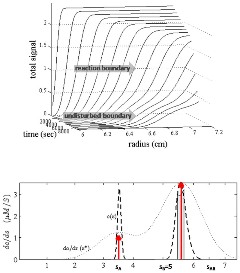
Top: Signal profiles a(r,t) of a rapidly reversible interacting system with 1:1 stoichiometry. Signal profiles are calculated from Lamm PDE solutions for a species A (3.5 S, 40 kDa) reversibly interacting with B (5 S, 60 kDa) to form transient complexes AB (6.5 S), sedimenting at 60000 rpm with equimolar loading concentrations at K_D. Bottom: Sedimentation coefficient distributions: an apparent velocity distribution g*(s*)~da/dr (grey dotted line); the diffusion-deconvoluted distribution c(s) (black dashed line); the asymptotic reaction boundary predicted by Gilbert-Jenkins theory (grey bar); and the predictions from EPT (red arrows).

Figure 7.

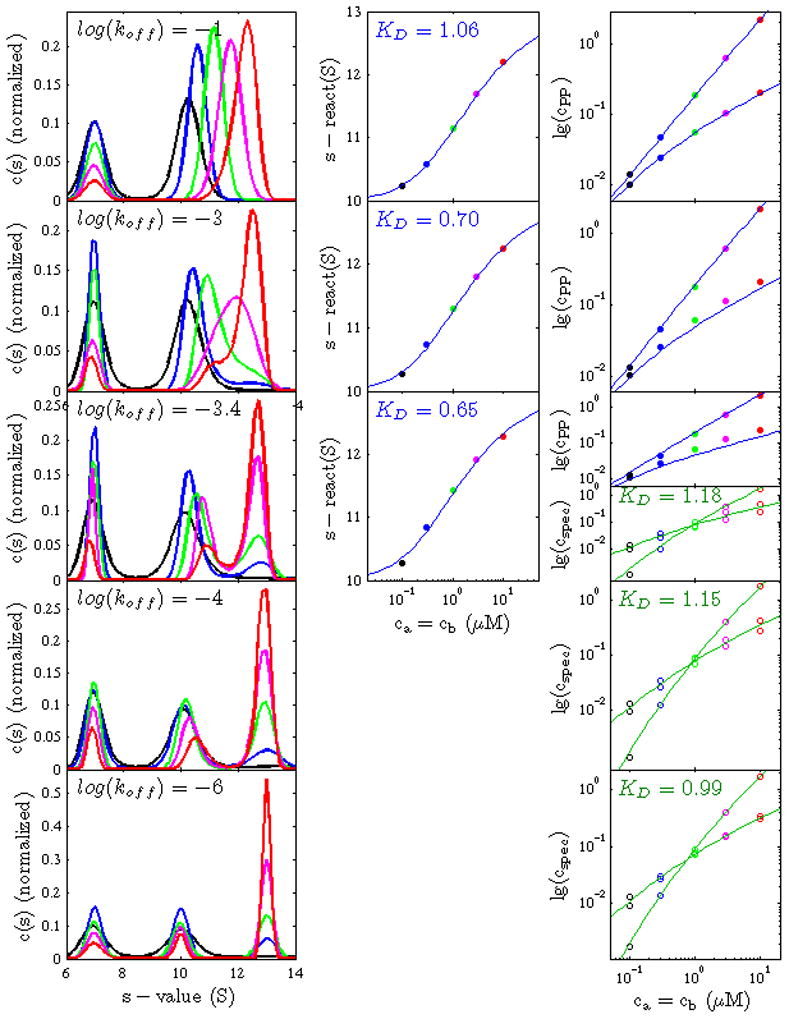
Effect of intermediate kinetics on the boundary structure and its analysis with the limiting models of EPT and mass action law. Left Panel: c(s) traces (normalized by the integrated area) derived from simulated SV data based on Lamm equation solutions for a 1:1 interaction, using equimolar loading concentration of 0.1 (black) 0.3 (blue) 1.0 (green) 3.0 (magenta) and 10 (red) fold K_D. The different columns show the data from simulations with different kinetic rate constants, with log₁₀(k_off) = −1, −3, −3.4, −4, and −6 (top to bottom). For the fastest and the slowest reaction kinetics, respectively, the characteristic boundary patterns can be discerned of two concentration-dependent or three concentration-independent c(s) peaks, respectively. These patterns morph at intermediate kinetics. Middle and Right Panel: For cases where the interpretation of a reaction boundary pattern is conceivable, c(s) was integrated (between 9 and 15 S) to determine the s-value of the reaction boundary (Middle Panels, solid circles), as well as to determine the signal amplitudes of the undisturbed and the reaction boundaries (Right Panels, solid circles). Both were globally fit (blue lines) with isotherms from EPT, with the result indicated in blue text labels. Alternatively, where three distinct peaks can be discerned that conceivably allow the application of the ordinary species analysis framework, the signal amplitudes of free A, free B, and complex AB were determined by integration of c(s) (Right Panel, open circles), and a mass action law model was globally fit (Right Panel, green lines), leading to results indicated in green text labels. In all analyses, errors in the total loading concentration were not considered.

Figure 8.

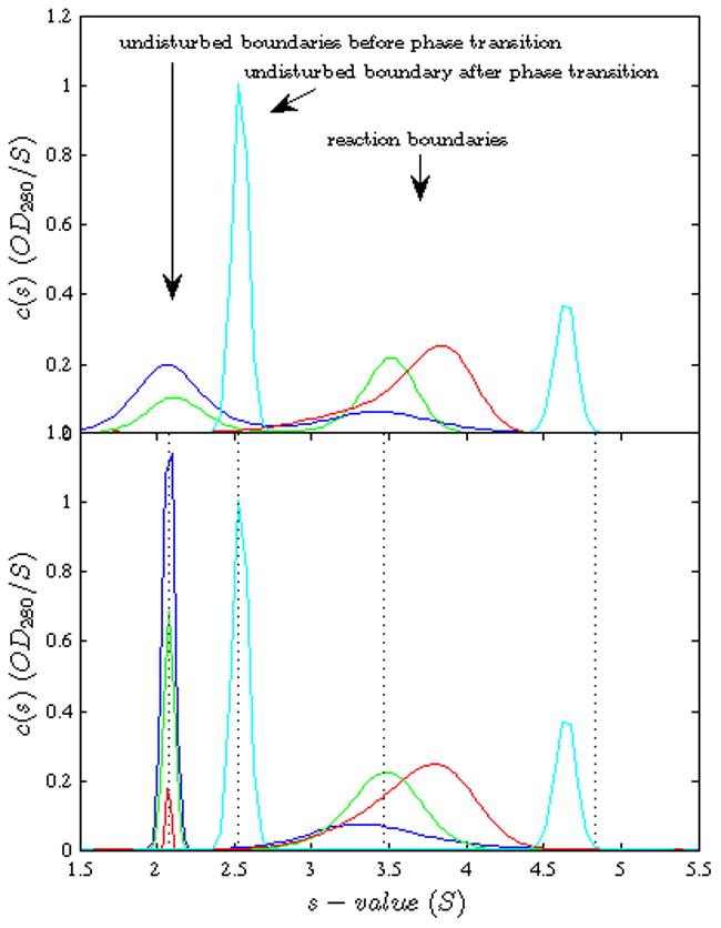
Experimental sedimentation coefficient distributions from a titration series of SBTI (~2.1 S) with increasing CT (~2.5 S). SBTI and CT were purchased from Worthington Biochemical (Lakewood, NJ), chromatographically purified and diluted into 50 mM Na/K phosphate, 150 mM NaCl, pH 7.4 buffer. Sedimentation experiments were carried out in a ProteomeLab XL-I analytical ultracentrifuge (Beckman Coulter Inc, Brea, CA) according to standard methods [58, 59] at 20°C and 59,000 rpm, recorded with absorbance optical system at 280 nm. Concentrations were constant 2.0 μM SBTI and 0.2 μM (blue), 0.6 μM (green), 2.0 μM (red), and 12.0 μM (cyan) of CT. Top Panel: First the standard c(s) analysis, with maximum entropy regularization at a confidence level of P = 0.68, was performed as described in [58]. Bottom Panel: In order to improve the separation of the peaks for precise integration, c(s) was recalculated with maximum entropy regularization enhanced with Bayesian prior knowledge of the s-values of the undisturbed boundary, also at a confidence level of P = 0.68. The vertical dotted lines indicate the s-values of both components (separately measured) and the best-fit s-values of the 1:1 and 2:1 complexes.

Only recently, the properties of these characteristic boundary features and their physical origin have been addressed by the effective particle theory (EPT) [45]. It is based on the simple physical picture of an ergodic reaction boundary where the time-average s-values of all molecules must match. Mathematically, this picture arises as a step-function solution of the Lamm equation of interacting systems, which can be motivated by the assessment of the net transport of each boundary component (see below). This leads to analytical expressions for the s-values and compositions of all boundary components. EPT models can be fitted to the corresponding quantities extracted from experimental SV data by c(s). EPT models can also be derived for higher-order association schemes, thus potentially aid in the characterization of more complex interactions.

The utility of EPT for qualitatively understanding and quantitatively analyzing SV experiments of heterogeneous interactions is the focus of the present work. To this end, we briefly review the existing approaches for the analysis of heterogeneous interacting systems by SV and their relationship to EPT. We will also introduce a new EPT-based tool in SEDPHAT facilitating the design of SV experiments of heterogeneous interactions.

Theoretical Background

Lamm equation modeling

DLEM is based on the use of Lamm equations for all chemical species coupled with discrete reaction schemes [20]:

$$\frac{\partial {\chi }_i}{\partial t}+\frac{1}{r}\frac{\partial }{\partial r}\left[r\left(s_i{\omega }^{2}r{\chi }_i-D_i\frac{\partial {\chi }_i}{\partial r}\right)\right]=q_i$$ (1)

where r is the distance from the axis of rotation, t the time after start of centrifugation, ω denotes the rotor angular velocity, and i enumerates the species participating in the interaction, with their molar concentration distribution χ_i (r, t) governed by sedimentation and diffusion coefficients s_i and D_i, respectively, and by the local chemical reaction flux between the species, q_i. In the special case that the fluxes are zero, Eq. 1 describes a set of Lamm equations of non-interacting discrete species, which can be solved most efficiently and precisely [40] with the adaptive grid algorithms [46] based on the finite element solutions introduced by Claverie [27]. In the simplest case of a bimolecular reaction between two species forming a 1:1 complex, q₁ = q₂ = −q₃ = −q with q = k_on χ₁ χ₂ − k_offχ₃, where k_on and k_off denote the chemical on-rate and off-rate constant, respectively, with the equilibrium dissociation constant K_D = k_off/k_on. Systems of Lamm equations Eq. 1 can be solved numerically for example using techniques described in [22, 24, 25], and fit to experimental data by non-linear regression.

Weighted-average sedimentation coefficients s_w

One of the earliest, most powerful, and still most commonly used approaches for the data analysis of interacting systems is the analysis of weighted-average (or signal-average) sedimentation coefficients s_w as a function of loading composition [5, 17, 18]. It is rooted in the measurement of the overall material transport across an imaginary plane in the solution plateau (at a radius r_p with the concentration a_p measured in signal units),

$$s_w=-\frac{1}{{\omega }^2{r}_p^2{a}_p}\frac{d}{dt}\underset{r_m}{\overset{r_p}{\int }}a(r,t)\mathit{rdr},$$ (2)

a consideration that is completely independent of the shape of the sedimentation boundary [5, 18]. It reflects only the average transport contributions from all species in solution, independent of their chemical interconversion kinetics.¹

Once s_w is determined (see below) for samples of different total loading concentrations c_k,tot of components k, an interaction model is used to fit the dependence of s_w on the solution composition with an isotherm

$$s_{w,\lambda }(\{c_{k,\mathit{tot}}\})=\frac{{\displaystyle \sum _i}{\epsilon }_{i,\lambda }{s}_i{c}_i}{{\displaystyle \sum _k}{\epsilon }_{k,\lambda }{c}_k}$$ (3)

composed of the contributions of all species i weighted with their signal coefficient ε_i and sedimentation coefficient s_i, at a molar concentration c_i predicted by mass action law. For heterogeneous interactions with spectrally distinguishable signals (for example, using UV absorbance at 250 nm and 280 nm, and/or interference optical signals), it is advantageous to carry this out as global fit to all s_w values from all signals λ. As a result, estimates for the equilibrium binding constants and the complex s-values can be obtained. Different binding models for the global fitting of s_w isotherms have been implemented in the software SEDPHAT.

By itself, unfortunately the s_w analysis of interacting systems suffers from the same drawback as many purely spectroscopic isotherm methods, in that all species in solution contribute to a single number derived from each experimental mixture, which then is deconvoluted into species contributions by fitting the isotherm with mass action law models. Problems can be the presence of contaminating species, as well as the finite information content of the isotherm from a necessarily limited concentration range for determining equilibrium constants and sedimentation coefficients for all complexes [18].

Sedimentation coefficient distributions c(s)

Rather than measuring s_w by assessing the rate of material transport directly from the raw concentration profiles, s_w is currently most often determined from the diffusion-deconvoluted sedimentation coefficient distribution c(s), which – as all successful direct boundary fits (irrespective of their physical motivation) – is faithful to the material transport and therefore rigorously relates s_w with the integral of the c(s) distribution [18]

$$s_w=\underset{s_{min}}{\overset{s_{max}}{\int }}c(s)\mathit{sds}/\underset{s_{min}}{\overset{s_{max}}{\int }}c(s)ds.$$ (4)

The sedimentation coefficient distribution c(s) is defined by the integral equation

$$a(r,t)\cong \int c(s){\chi }_1(s,M(s),r,t)ds,$$ (5)

which is to be fit to the experimental data a(r,t) [38]. c(s) has the units of signal/S. In Eq. 5, χ₁(s, M (s), r, t) is the ideal sedimentation profile of a single discrete, non-interacting species, and M(s) is a hydrodynamic scaling law. For compact proteins, it is usually based on s ~ M^2/3 [38] with a best-fit average frictional ratio f/f₀, but it is easy to see that other scaling laws with different conformational factors are more useful for other types of macromolecules [47, 48] (a variety of models are implemented in SEDFIT). The scaling law also allows the stable transformation of the sedimentation coefficient distribution c(s) into a molecular weight distribution c(M).

For multi-signal analysis, the sedimentation coefficient distribution takes the form

$$a_{\lambda }(r,t)\cong \sum _k{\epsilon }_{\lambda k}{l}_{\lambda }\int c_k(s){\chi }_1(s,M(s),r,t)ds$$ (6)

where data a_λ at signals λ (acquired with optical pathlength l_λ) are globally fitted with sedimentation coefficient distributions of component k, with (usually predetermined) extinction coefficients ε_λk [6, 10, 34]. c_k(s) has the units of molar concentration/S.

As shown in [41], the decomposition of experimental data Eq. 5 into a c(s) distribution can also be applied to slowly as well as rapidly interacting systems. When the integration limits s_min and s_max in Eq. 4 are chosen such as to encompass the reaction boundary, excluding the undisturbed boundary (see below), the result will be termed s_fast [45]. As mentioned above, when they encompass all sedimenting species, the result is identical to s_w as defined in Eq. 2. This route for determining s_w and s_fast provides one with 1) the choice to exclude non-participating species forming separate sedimentation boundaries from consideration in determining s_w and s_fast; and 2) the opportunity to determine from the actual sedimentation profile the loading concentrations of interacting species (provided extinction coefficients or other signal coefficients are available) and the signal amplitude of the reaction boundaries.

The boundary structure, especially when deconvoluted from the effects of diffusion in c(s), can allow the assessment whether the interaction is slow on the time-scale of the sedimentation experiment, i.e. typically with a complex half-life exceeding ~10,000 sec, or if it is equilibrating fast, i.e. typically with a complex half-life less than 1,000 sec: Fast reactions show a concentration-dependence of the s-value of the boundaries, whereas slow reactions show concentration-independent boundary velocities (e.g., see Figure 7 below). For the majority of cases, this provides all the kinetic information from the AUC experiment that can be reliably extracted. Qualitative knowledge on the time-scale of the interaction offers two alternative paths for further analysis.

1. When the reaction is slow relative to the sedimentation, hydrodynamic separation of all species occurs, and a simple quantitation of all species’ concentrations with the help of the sedimentation coefficient distribution c(s) can be interpreted directly with mass action law models². In this case, little extra information could be gained by Lamm equation modeling.

   In fact, valuable information on the complexes formed can be gained from the c(s)/c(M) analysis even without an existing hypothesis for the mechanism of complex formation: Under conditions of very slow reactions, or when the complex formation is virtually saturated by component concentrations in very large excess over the equilibrium dissociation constant K_D, the complex will trivially behave like a noninteracting species and can be characterized as such, for example, by interpreting the molecular weight implied by c(s) and the best-fit f/f₀ (which is equivalent to the use of c(M)). Further, for slow systems, the multi-signal sedimentation coefficient distribution c_k(s) also provide direct information about the composition of each (resolvable) species, irrespective of the reaction scheme.

2. In many cases of interacting systems accessible to the study by SV, the reaction kinetics is fast relative to the sedimentation time. In this case, the experimental boundary structure is simpler, exhibiting only two boundaries for two-component systems (or generally up to n boundaries for n-component systems). But the interpretation is more complex, since the fast boundaries represent reaction boundaries with properties that are governed by all species concentrations and s-values, as well as the binding constants.

Effective particle theory

For fast systems, it is essential to recognize that not all boundaries reflect the sedimentation of directe chemical species, but that one of the boundaries always reflects the propagation from the coupled sedimentation and chemical reaction process. The salient characteristics of the boundary pattern and boundary properties can be derived from a diffusion-free picture, as shown in EPT [49]. EPT is based on the approximation of each of the boundaries with Heaviside step-functions rather than diffusionally broadened profiles. This is motivated by the focus on the transport arising from each boundary through an imaginary plane in the plateau region, analogous to the migration of equivalent boundary position defined by s_w for the overall transport. When the step-functions are inserted into the partial differential equation Eq. 1 with all D_i = 0, simple algebraic relationships are obtained in the framework of generalized functions (for the detailed derivations, see [49]). These relationships will be outlined in the following for a 1:1 reaction with an equilibrium association constant K, but can be extended for higher associations with multi-site binding [49], as well as mixed self-association/hetero-associating systems (unpublished results).

For the sedimentation coefficient of the reaction boundary, s_A···B, it is

$$s_{A\cdots B}=\frac{c_X{s}_X+c_{AB}{s}_{AB}}{c_X+c_{AB}}\mathit{with}\{\begin{array}{cc}X=A& \mathit{for}{c}_{\mathit{Btot}}>c_{\mathit{Btot}}^{\ast }\\ X=B& \mathit{else}\end{array},$$ (7)

where X denotes the component that is sedimenting entirely in the reaction boundary, and c_X and c_AB denote here the molar free and complex concentrations, respectively, predicted from mass action law for the initial equilibrium at rest. Which component is entirely in the reaction boundary is not determined by molar excess, but by an asymmetric phase transition line in the plane of total concentrations: If we denote A and B the slower and faster sedimenting component, respectively, such that s_A < s_B (both s_A and s_B are assumed positive in EPT, excluding flotation), then X is equal to the slower sedimenting component A if the total loading concentration c_B,tot of the faster sedimenting component B exceeds

$$c_{B,\mathit{tot}}^{\ast }(c_{A,\mathit{tot}})=c_{A,\mathit{tot}}+\frac{(s_B-s_A)}{2K(s_{AB}-s_B)}\left(1+\sqrt{1+\frac{4c_{A,\mathit{tot}}K(s_{AB}-s_B)}{(s_{AB}-s_A)}}\right),$$ (8)

otherwise X is equal to the faster sedimenting component B. For this transition, in the limit of very low concentrations of A, we obtain

$$c_{B,\mathit{tot},min}^{\ast }=\frac{(s_B-s_A)}{K(s_{AB}-s_B)}.$$ (9)

If we denote Y the remaining component that is partitioning both into the reaction boundary and the undisturbed boundary, one obtains the expression

$$c_{Y,\mathit{undist}}=c_{\mathit{Ytot}}-c_{AB}\left(1+\frac{(s_{AB}-s_Y)}{K{c}_Y(s_{AB}-s_Y)+(s_X-s_Y)}\right)$$ (10)

for the concentration of the undisturbed boundary, which will be sedimenting with s_Y. The remaining unbound material of Y, (c_Y,tot – c_Y,undist) is co-sedimenting in the reaction boundary, along with all of free X and all of the complex XY.

It was shown that Eq. 7 – 10 ensure the ergodicity of the reaction boundary, in a sense that the fractional time that molecules of each component are either free or bound results in an average velocity that matches (for both components) the velocity of the reaction boundary [49]. This can be visualized as an effective particle with fractional states A, B, and AB that sediments in a dynamically concerted fashion as depicted in Figure 2.

Figure 2.

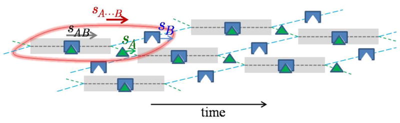
Cartoon of the effective particle A···B (encircled in red). Indicated is the fractional time that A (green) and B (blue) spend free or in complex (greyed time intervals). The representation is faithful with regard to relative concentrations, velocities, and species lifetimes. Component A spends a smaller fraction of time free than B, resulting in a match of their time-average velocities. An animation can be found at [50].

The composition of the effective particle, R_A···B = c_X,0/(c_AB + c_Y,0 − c_Y,undist), that would be measured in a multi-signal SV experiment, is

$$R_{A\cdots B}=\{\begin{array}{cc}1-(s_B-s_A)/K{c}_B(s_{AB}-s_B)& \text{for}{c}_{B,\mathit{tot}}>c_{B,\mathit{tot}}^{\ast }(c_{A,\mathit{tot}})\\ 1-1+K{c}_A(s_{AB}-s_A)/{(s_B-s_A)}^{-1}& \text{else}\end{array}$$ (11)

An extension of EPT [41] allows to predict the diffusional spread of the reaction boundary

$$D_{A\cdots B}\approx \frac{c_X\frac{D_X{c}_X+D_{AB}{c}_{AB}}{c_X+c_{AB}}+(c_Y-c_{Y,\mathit{undist}})\frac{D_Y(c_Y-c_{Y,\mathit{undist}})+D_{AB}{c}_{AB}}{(c_Y-c_{Y,\mathit{undist}})+c_{AB}}}{c_X+(c_Y-c_{Y,\mathit{undist}})}$$ (12)

from which, we can operationally assign an apparent molecular weight to the effective particle, in analogy to the Svedberg equation,

$$M_{A\cdots B}(1-\overline{v}\rho )=\frac{s_{A\cdots B}RT}{D_{A\cdots B}}$$ (13)

This approximates the apparent molecular weight that would be observed in c(M) (where the partial-specific volumes of A and B are assumed to be similar and v̄ is taken as their average). The apparent molecular weight associated with the boundary spread it is higher than the total weight-average molecular weight but smaller than the complex molecular weight M_AB. However, due to the approximate nature of M_A···B, the main focus of our use of EPT in the present work is the dependence of the s-values of the undisturbed and reaction boundaries, as well as their composition, as a function of total loading concentration.

Results

Examples for the boundary structure of different systems

Figure 3 shows examples for the boundary patterns calculated via Eqs. 7 – 12 for a rapid reaction with 1:1 stoichiometry. The two columns of panels display EPT isotherms for different properties as a function of total A and B (using a nomenclature where the slower sedimenting component is designated ‘A’, the faster sedimenting one ‘B’) calculated on the left column for similar-sized particles (M_A = 75 kDa, s_A = 4.9 S, M_B = 80 kDa, s_B = 5.0 S, s_AB = 7.5 S) and on the right column for very dissimilar-sized particles (M_A = 5 kDa, s_A = 0.8 S, M_B = 80 kDa, s_B = 5.0 S, s_AB = 5.3 S). Shown are (top to bottom) the s-value, composition, and scaled molecular weight of the reaction boundary, followed by the s-value and relative concentration of the undisturbed boundary. Figures 4 and 5 show a comparison of s_w, s_A···B, and the stoichiometry R_A···B of similar-sized (Figure 4) and dissimilar-sized (Figure 5) components for reactions of different stoichiometry.

Figure 3.

Boundary patterns predicted by EPT for similar-sized particles with M_A = 75 kDa, s_A = 4.9 S, M_B = 80 kDa, s_B = 5.0 S, s_AB = 7.5 S (Left Column) and for dissimilar-sized particles (M_A = 5 kDa, s_A = 0.8 S, M_B = 80 kDa, s_B = 5.0 S, s_AB = 5.3 S) (Right Column). Each panel displays a contour plot of an isotherm of the property indicated in the label as a function of total A and B (with s_A < s_B), with a color temperature scaled to the property values as shown in the color bar. The phase transition line is shown as dashed black line.

Figure 4.

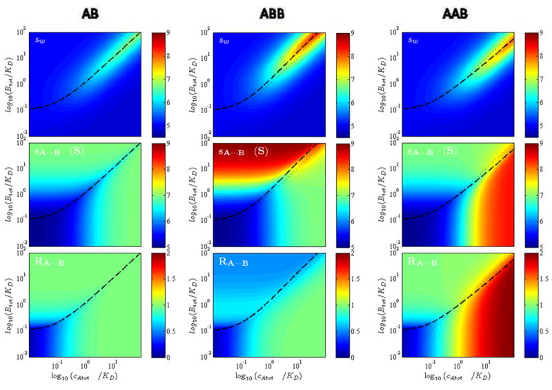
Boundary patterns predicted by EPT for similar-sized particles for reactions with different stoichiometry: 1:1 (Left Column), 1:2 (Middle Column), and 2:1 (Right Column). Shown are isotherms in the form of color contour plots for the weight-average s-value (Top Row), the s-value of the reaction boundary (Middle Row), and the composition of the reaction boundary (Bottom Row). Calculations are with M_A = 75 kDa, s_A = 4.8 S, M_B = 80 kDa, s_B = 5.0 S, s_AB = 7.0 S, s_AAB = 8.5 S, s_ABB = 9.0 S; for two-site models equivalent non-cooperative binding constants were assumed. The phase transition line is shown as bold dashed line, the equimolar line as thin dotted diagonal line from bottom left corner to the top right corner.

Figure 5.

Boundary patterns predicted by EPT for dissimilar-sized particles for reactions with different stoichiometry: 1:1 (Left Column), 1:2 (Middle Column), and 2:1 (Right Column). The presentation is analogous to Figure 4. Shown are isotherms in the form of color contour plots for the weight-average s-value (Top Row), the s-value of the reaction boundary (Middle Row), and the composition of the reaction boundary (Bottom Row). Calculations are with M_A = 5 kDa, s_A = 0.5 S, M_B = 80 kDa, s_B = 5.0 S, s_AB = 5.3 S, s_AAB = 5.5 S, s_ABB = 8.0 S; for two-site models equivalent non-cooperative binding constants were assumed. The phase transition line is shown as bold dashed line, the equimolar line as thin dotted line.

The isotherms have many noteworthy features. Among the most striking is the asymmetry of the phase transition in the parameter space of loading concentrations. By no means is the component providing the undisturbed boundary simply that in molar excess: this is true only in the limit of equally sized component (s_A = s_B). Generally, it takes a larger excess of the larger component (B) in order to drive the smaller component (A) fully into the reaction boundary. This is required such as to increase the fractional saturation of A and allow the time-average velocity of A in the reaction boundary to be at least that of free B (since the condition s_A···B < s_B cannot exist). For smaller A, this takes higher saturation. As a consequence, the asymmetry of the phase transition increases with the asymmetry of the particle sizes. Its location can provide information on K_D and s_AB. Interestingly, from inspection of Figure 4 and 5 we can discern that it is strongly dependent on the reaction stoichiometry only for dissimilar-sized particles.

Another interesting feature is the composition of the reaction boundary. It was shown in EPT that it must always be smaller than the complex stoichiometry, across the whole parameter space of loading concentrations. This is due to the smaller population of free A than free B co-sedimenting in the reaction boundary. However, for similar-sized particles we find that, with the exception of very low concentrations of both components, the composition of the reaction boundary is always close to the true stoichiometry of the complexes formed. This observation is important for the application of multi-signal c_k(s) to determine the maximum complex stoichiometry in uncharacterized systems. (An obvious caveat is that for multi-site binding the type of complex that predominates will depend on which component is in excess.) For dissimilar sized particles, it is interesting that a 10-fold molar excess of c_A,tot over K_D will always lead to an excellent estimate of the stoichiometry of the complexes formed, even for very low concentrations of B. (The reverse is not true.) When working with dissimilar-sized particles, this will make it easier to determine spectroscopically the maximum content of the smaller component A in the complex.

It is often important to experimentally define the s-value of the complex well, either for the purpose of hydrodynamic modeling, or simply to arrive at a better conditioned analysis of the binding constants [18]. Different from the question of reaction stoichiometry, the determination of the complex s-value requires at least partial saturation of the reaction boundary, such that s_A···B approaches s_AB. For 1:1 reactions, this requires either ~10-fold molar excess of A over the binding constant, c_A,tot > 10 K_D (preferably at low concentrations of B), or, in the opposite configuration, a 10-fold molar excess of B over the phase transition line, i.e. c_B,tot > 10 K_D(s_B-s_A)/(s_AB-s_B) (preferably at low concentrations of A). It is noteworthy that these conditions are more stringent than those for obtaining the complex composition.

If we had to rely solely on s_w for determining either the complex s-values or stoichiometries (which are also required for the well-conditioned determination of K_D), as can be discerned from the top rows in Figure 4 and Figure 5, it would be necessary to essentially saturate complex formation in solution, i.e., force the complex to be the major populated state by using high concentrations of both A and B. This is often much more difficult to achieve, due to limitations in available material and in the stability of the components at high concentrations. Thus, it is highly advantageous in many respects to utilize the hydrodynamic resolution of the boundary structure, and especially to characterize the reaction boundary that forms as a very distinct feature even at low sample concentrations.

Using EPT to design experiments with the effective particle explorer in SEDPHAT

The relative simplicity of EPT makes it easy to predict all observables of the boundary structure given component s-values and extinction coefficients (which can presumably be determined in independent experiments), and given hypothetical complex s-values and binding constants. This can aid in the experimental design. For this purpose we have implemented the Effective Particle Explorer tool in the public domain software SEDPHAT. It displays for different association models all experimental observables of the boundary structure as a function of total loading concentrations, including the s-value of the reaction boundary and the undisturbed boundary, the composition and apparent molecular weight of the reaction boundary, the relative concentration of the undisturbed boundary, the signal ratio of the undisturbed vs reaction boundary, and the overall weighted (signal) average s-value. Further, for 1:1 association models, animated cartoons of the reaction boundary can be displayed (analogous to the movies [49, 50]) in order to visualize the propagation of the reacting system and the dynamic process of coupled sedimentation and association/dissociation.

For the practical design of experiments, the sample concentrations are always limited, either trivially from availability of material, or due to the intrinsic stability of the components with regard to aggregation. This implies constraints in the accessible concentration range of mixtures in the isotherm shown in Figures 3 – 5. Other practical limits can be imposed by the need to avoid significant hydrodynamic non-ideality, restricting the total mg/ml concentration in the samples. Similarly, the absorbance optical signal imposes maximum signals for which the detection remains sufficiently linear. Likewise constraining the accessible range over which the isotherms can be probed is the minimum signal that is reliably detectable and still allows resolving the boundary structure (it may be set, for example, at 0.05 OD). Accordingly, the user can enter the minimum and maximum mg/ml concentrations, as well as minimum and maximum desired signals (along with the components’ extinction coefficients), and the isotherm will be cropped to the accessible region.

Such a cropped isotherm is shown in Figure 6, for the interacting system of Figure 1, assuming a binding constant of K_D = 1 μM, extinction coefficients for A and B of 50,000 and 100,000 OD/Mcm, respectively, with 1.2 cm pathlength for standard centerpieces. The stock concentration were assumed to be 3 mg/ml and 5 mg/ml for A and B, respectively, the minimal signal was set to 0.05 OD, and the maximum signal was set to 1.5 OD.

Figure 6.

Screenshots of the SEDPHAT Effective Particle Explorer, showing the accessible range of concentrations of the isotherms of the reaction boundary s-value s_A···B (Top), the signal-average s-value s_w (Middle), and the s-value of the undisturbed boundary (Bottom) for the system of Figure 1. The black areas indicate concentrations inaccessible with the constraints of available total concentrations of 3 and 5 mg/ml of A and B, respectively, minimal signals of 0.05 OD, and maximal signals of 1.5 OD, respectively. The black circles connected with solid black lines are proposed concentrations, equally spaced on a log-scale, in this example keeping the total molar concentration constant (like in a Job analysis).

In order to further facilitate experimental planning, it is possible in this tool to indicate rational experimental series (such as titration, dilution, Job, or linear relationships on a log(c_A,tot)-log(c_B,tot) scale). This can be accomplished in this SEDPHAT window by moving the computer mouse along a line across the accessible isotherm range while keeping the right mouse button depressed. The goal is to indicate the trajectory probing the isotherm of the most informative observable for a given problem. In return, SEDPHAT will propose rational equidistant (on a log-scale) experimental concentration pairs along this trajectory, in a total number determined by the user (e.g. seven when using a eight-hole rotor with counterbalance). Furthermore, a text file will be created and opened in a separate notepad window (not shown), describing a detailed pipetting plan for generating these samples with given stock concentrations of sample and buffer for dilution, and also reporting the total stock volumes and mg quantities of each component needed for the experimental series.

Which trajectory(ies) will be optimally selected depends on the focus of the study (see above). For example, when the stoichiometry of the interaction is unknown, it is possible and prudent to hypothesize different models and select trajectories that sample isotherm regions that experience the maximum change with different association models, and isotherm regions would be expected to exhibit reaction boundary compositions close to the stoichiometry. In any case, the accessible isotherms shown in Figure 6 reinforce the notion that the signal weighted-average s_w-value (Middle Panel), which is the traditional quantity to be analyzed from the experiment, is far less informative than the combination with the s-values (and signal amplitudes) of the undisturbed and the reaction boundary.

The effect of finite reaction kinetics on the boundary structure

EPT was derived from the Lamm equations (Eq. 1) under the mathematical special cases of negligible diffusion and of infinitely fast reaction kinetics. In practice, it may not always be clear whether or not an interaction can be considered infinitely fast on the time-scale of sedimentation. The typical transition of reaction kinetics exhibiting ‘slow’ or ‘fast’ sedimentation behavior has been found to take place in a narrow range of kinetic off-rate constants between 10⁻⁴/sec and 10⁻³/sec [24]. In order to study the effect of finite complex lifetimes on the boundary structure, we have simulated Lamm equation solutions of 1:1 interactions with log(k_off) of −1 (which can be considered infinitely fast in the context of SV), −3 (still fast, but on the limit where kinetics should significantly influence the boundary pattern), −3.4 (intermediate), −4 (in the slow regime, but still influenced by kinetics), and −6 (essentially infinitely slow on the SV time-scale). For loading concentrations, we simulated an equimolar dilution series (Figure 7).

Corresponding to the first step in SV analysis, the first column of Figure 7 shows the diffusion deconvoluted sedimentation coefficient distributions c(s), highlighting the boundary pattern (Left Column). For fast kinetics (First Row), as expected, we see the bimodal division into the undisturbed and the reaction boundary with the tell-tale sign of concentration-dependent peak s-value, which can be analyzed in the framework of EPT on the basis of s_A···B (Middle Column) and the undisturbed and reaction boundary amplitudes (Right Column, blue lines). In the other extreme, for slow kinetics (Bottom Row) we see the trimodal boundary pattern resolving each sedimenting species A, B, and AB at constant peak s-value (Left Column). The amplitudes of each boundary component can be modeled directly by mass action law³ (Right Column, green lines).

Slightly broader c(s) peaks can be discerned at log(k_off) of −3 and −4 (second and fourth row, respectively). Importantly, no new phenomenology occurs, even for intermediate kinetics log(k_off) of −3.4 (Third Row): Here, intermediate, not baseline-resolved peaks occur, which could be interpreted either as seemingly sub-structured concentration-dependent peaks and interpreted in the context of EPT (Middle and Right Panel, blue lines), or they could be regarded as separate peaks and interpreted as species populations (Right Panel, green lines). Interestingly, the boundary can also be quantitatively fit either way with very moderate errors. In EPT, this case would lead to a 0.65-fold underestimate of K_D, whereas in the slow interpretation an ~1.2-fold overestimate would occur. Thus, from this example it seems that errors from applying EPT to systems with finite kinetics can remain, even for extreme cases, within approximately a factor two for the binding constant. Similar results are obtained for analogous simulations along a titration series crossing the phase transition line (data not shown).

Even smaller errors were obtained for the application of species population isotherms based on mass action law. This analysis is strictly correct in SV only for infinitely slow interactions. When the kinetic off-rate constant is small but non-zero, slight overestimates of the K_D were observed (Figure 7), increasing with faster kinetics. An interesting tell-tale for the finite kinetics is the difference of the concentration of free A and free B measured despite the equimolar loading concentrations. This discrepancy cannot be explained by mass action law, and is a result of asymmetric co-migration of free species in the reaction boundary.

Experimental Results

In order to study the boundary structures experimentally, we performed SV experiments with α-chymotrypsin (CT) and soybean trypsin inhibitor (SBTI), which interact to form 1:1 and 2:1 complexes [51]. The top panel of Figure 8 shows c(s) profiles calculated in SEDFIT of an experimental titration series of SBTI with increasing concentrations of CT, calculated with standard maximum entropy regularization at a confidence level of P = 0.68. From the first qualitative inspection we can discern the undisturbed boundaries of SBTI at low concentrations of CT (blue and green traces), a trace with seemingly no undisturbed boundary (red), and a trace with an undisturbed boundary of CT (cyan). In all experiments, we can recognize a reaction boundary at different s-values.

The first step for the quantitative comparison of the boundary structure with EPT is the integration of c(s) to determine the overall signal-average s_w, the signal average s-value of the reaction boundary, and the amplitudes of the undisturbed and reaction boundaries. For data sets with relatively small molecules, the hydrodynamic separation may not produce baseline-separated peaks. This is exacerbated at low signal-to-noise ratios by the effect of the standard maximum entropy or Tikhonov regularization reporting the broadest possible peaks that fit the data within a certain confidence level. This effect could be observed here, for example, as shown in the blue trace. However, having knowledge of independently determined s-values of the free species, and the theoretical background that the undisturbed boundary should migrate with the s-value of the free species, we can deviate from the default maximum entropy regularization and utilize our knowledge in the form of a Bayesian prior [52]. The resulting distribution is termed c^(P)(s), to emphasize the dependence on the particular prior. By design of the Bayesian distribution analysis in SEDFIT, the c^(P)(s) fit the raw data strictly equally well as c(s), but accommodate our prior knowledge as much as possible for the given noise of the data [52]. In the present case, the prior knowledge was implemented in the form of a Gaussian centered at the pre-determined s-value of the species providing the undisturbed boundary, but this could equally well be accomplished by using as a probability distribution the pre-determined c(s) trace of the individual component.⁴ This resulted in the c^(P)(s) traces shown in the Bottom Panel, and the baseline-separated peaks that could be unambiguously integrated.⁵

In the same way, we performed and analyzed experiments from a series with approximately constant molar ratio of 1.9:1, and a single experiment with low concentration of SBTI (0.1 μM) and a very large excess of CT (10 μM). Tools for global fitting and plotting of isotherms were implemented in SEDPHAT, and all data were included in a global isotherm analysis shown in Figure 9. The top panel shows the boundary amplitudes, with the reaction boundary and its best-fit isotherms with solid symbols and solid lines, respectively, and the undisturbed boundary signals as open symbols and dotted lines, respectively. The phase transition with the vanishing undisturbed boundary appears as a singularity in this log-log plot, as visible in the dotted blue line and open blue symbols from the titration series that crosses the phase transition line. The middle panel displays the s_fast-values, i.e. the c(s) signals integrated across the reaction boundary (solid circles) and the best-fit isotherms (solid lines). The lower panel, finally, displays the conventional weighted- (signal-) average s-values from the integration of all c(s) boundaries (open circles). Obviously, the reaction boundary s_fast-values are higher throughout. Interestingly, a very steep isotherm is obtained for the titration series where s_w exhibits a broader transition through a maximum. Also, a noteworthy comparison is the single data point from the experiment with large molar excess (green symbols), which is extremely useful to saturate complex formation as much as possible and to obtain a c(s) peak at an s-value close to that of the highest complex. In the s_w isotherm, this point is not very informative, since s_w is overwhelmed with the low s-value of the free species. While previously this information could only have been qualitatively interpreted, EPT now allows the rigorous inclusion of this information into the quantitative analysis.

Figure 9.

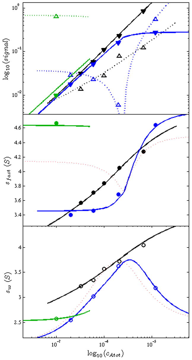
Global EPT isotherm analysis of the SBTI – CT interaction, incorporating the titration series data shown in Figure 8 (blue), a series of concentration pairs at a CT/SBTI ratio ~ 1.9:1 (black), and a single experiment with 100-fold excess of CT (green). Top Panel: Amplitudes of the reaction boundary (solid triangles) and undisturbed boundaries (open triangles) with best-fit isotherms (solid and dotted lines for reaction and undisturbed boundaries, respectively) as predicted by Eq. 10. Middle Panel: s-values of the reaction boundaries (solid circles), fitted with s_A···B of Eq. 7 (solid lines). Bottom Panel: Overall signal-average s-values, fitted with s_w from Eq. 3. In the Middle Panel and Bottom Panel, the best-fit isotherms from an impostor 1:1 model are shown as red dotted lines.

When fitting these isotherm data including the boundary amplitudes, an important point to consider is our usually imperfect knowledge of the exact protein concentrations. For this reason, it is common practice to treat the protein concentrations as floating parameters in DLEM. Just like in the analysis of sedimentation equilibrium (SE) experiments [53] as implemented in SEDPHAT, it is possible and highly useful in DLEM to condense the number of unknowns to those of the stock solutions when experiments are carried out in titration series or at constant molar ratio. In contrast, in isotherm analyses the protein concentrations are typically taken as known parameters. However, when including isotherms of boundary signal amplitudes into the global isotherm analysis, it is important to account for concentration errors, in complete analogy to direct boundary modeling. We have embedded this in SEDPHAT as a possibility to multiply the column of concentrations of either one of the components with a correction factor (obviously it should not be applied to both components at the same time). Its expectation value is 1.0 for perfectly known concentrations. In the best-fit result of Figure 9, an error of ~12% in the initially assumed concentrations of CT is estimated, assuming the extinction coefficients to be correct.

We compared the statistical uncertainties of the parameter estimates in the global model of Figure 9 with those from a conventional analysis of s_w isotherms only. While for the AB complexes (treated as indistinguishable) the global EPT analysis only provided an improvement of 4% in the uncertainty of the s_AB-value, a 2.1-fold reduction of the uncertainty for the ABB complex was observed. For the binding constants, with EPT we obtained a 1.5-fold reduction in the 95% confidence range of the macroscopic K_AB, and a 2.5-fold reduction of the uncertainty in the macroscopic cooperativity factor.

The best-fit estimates for the macroscopic dissociation equilibrium constants were in good agreement with those measured independently in parallel on the same preparation and under the same buffer conditions by other biophysical techniques, including isothermal titration calorimetry, surface plasmon resonance, and fluorescence anisotropy, and we will describe their global multi-method fit in a forthcoming communication (Zhou et al., manuscript in preparation).

Discussion

EPT can be derived as a special-case solution of a system of Lamm partial differential equations of interacting systems [49]. We have previously shown how EPT provides an intuitive physical framework for understanding the boundary structures exhibited in SV of rapidly interacting heterogeneous macromolecular systems [49]. In the present work, we have further explored how EPT may be used in the experimental design and in the quantitative data analysis.

With regard to the experimental design, the analytical simplicity of EPT allows to easily make predictions for the observables across the entire range of loading concentrations. With the implementation of the Effective Particle Explorer tool in SEDPHAT, besides making the physical process of reactive co-migration more transparent and intuitively accessible, we aimed at exploiting this potential to streamline the planning of experiments, and to allow a more rational choice of concentration parameters dependent on practical constraints and the particular focus of the experiment. Interestingly, conditions that reveal the reaction stoichiometry well encompass a wide fraction of the parameter space, but may not always be the most informative for determining binding constants or hydrodynamic properties of the complexes.

The isotherms shown in Figures 4 to 6 illustrate the well-known fact that much more information resides in the SV experiments than reflected in the isotherms of weighted-average s-values. The pattern of undisturbed and reaction boundary can usually be easily recognized and quantitatively extracted from the raw data, for example, through a c(s) analysis or other tools. In contrast, the quantitation of the spread of each boundary, and its interpretation in terms of simultaneous diffusion, heterogeneity, and chemical reaction, is much more difficult and requires more parameters and assumptions. EPT provides a framework to model the boundary patterns in terms of amplitudes and s-values, disregarding their shapes.

An obvious limitation of the EPT analysis is the assumption of fast reactions on the time-scale of the SV experiment. A hallmark of these reactions is the concentration-dependence of the s-value of the fast boundary, which can usually be easily recognized and distinguished from concentration-independent peak positions which are a signature of slow reactions on the time-scale of sedimentation. Only a relatively narrow range of kinetic constants fall in between these two cases. In this transition region, the c(s) analysis of the boundary patterns shows less concentration-dependence than fast systems and substructures of the boundaries. As illustrated in Figure 7, there is a continuous transition where the boundary patterns show both fast and slow features. In order to explore the sensitivity of the EPT analysis to the assumption of fast kinetics, we applied it to impostor simulated sedimentation data with such intermediate kinetics. Importantly, we did not find strongly diverging results when approaching the regime of intermediate kinetics. Instead, even when applied to data sets with already clearly established species boundaries, we obtained binding constants that were still within less than a factor two of the correct values, which is often within the 95% confidence interval of experimentally determined binding constants. At least, even in the worst-case scenario, the EPT results would provide excellent starting guesses for DLEM modeling, which would be most (or probably only) profitable in this intermediate kinetic regime. Fortunately, we would expect that overlay of c(s) traces such as in Figure 7 would allow us to discern the presence of intermediate kinetics and avoid significant errors from this source. Slightly faster reactions would bring the errors to a similar magnitude as common concentration errors.

Interestingly, as the reactions get slower and approach the intermediate regime, the most noticeable deviation from the EPT model is the amplitude of the undisturbed boundary, which becomes higher as less co-sedimentation of the slowest species in the reaction boundary takes place, as well as the s-value of the reaction boundary, which becomes faster as a result of less complex dissociation (and less co-sedimenting free material). In this way, the reaction kinetics is reflected to some extent in the boundary structure, although not exploited in the models studied here.

A second theoretical limitation arises from the neglect of EPT to account for changes in the reaction boundary composition within the radial range of the spreading boundary. We have previously shown that s_A···B from EPT is generally in excellent agreement with the average properties of the reaction boundary as predicted by Gilbert-Jenkins theory [49]. However, the largest deviations were found close to the phase transition line [49]. Therefore, data points very close to or at the phase transition line would not be expected to be perfectly modeled by EPT. On the other hand, at the phase transition point s_A···B becomes identical to s_w and the reaction boundary amplitude becomes trivially the loading concentration, such that the added information content of such data points for EPT may not be so great. However, the location of the phase transition line and the characteristic features surrounding it will have considerable value.

In the practical analysis of our model system of CT interacting with SBTI, we found very good agreement of EPT with the measured boundary patterns within the experimental errors. Notably, this even includes one data point from the titration isotherm in relative vicinity of the phase transition (Figure 8, red). Similarly high quality agreement was already previously reported for different systems, including the interaction of mouse CMV proteins with RAE-1 molecules [54], and for the interactions of Ly49 killer cell receptors with MHC molecules [55]. In the present study, we have considered some practical methodological aspects in more detail.

First, dependent on the s-values of the free species and the complex, it may not always be possible to resolve the undisturbed and reaction boundary well enough for satisfactory quantitative integration. Especially in this case, it is very useful to exploit the diffusional deconvolution of c(s), which was shown theoretically and practically to work remarkably well even for reaction boundaries [41]. However, limitations still occur, for example, for systems with small s-values which inherently have lower resolution, for systems with very dissimilar-sized molecules where the reaction boundary may not be well resolved from the undisturbed boundary of B above the phase transition, and generally for conditions of extremely low signals where the standard regularization causes broad peaks.

Recalling that the standard maximum entropy regularization is based on the preference, among all possible c(s) distributions that fit the data equally well, to report those that have the least preference for any particular s-value, it is prudent to adjust this regularization here such as to give preference to distributions that have peaks at the known s-value of the expected undisturbed boundary. The latter s-value is known from independent measurement of the free components. We can easily embed this knowledge using the Bayesian regularization tool of SEDFIT [52], either directly using an experimentally determined c(s) distribution as prior probability, or defining a Gaussian probability distribution around the mean s-value of the free components. As shown in the present example, this will facilitate the discrimination of the boundary patterns and their integration by promoting baseline-separated peaks. From a statistical point of view, this is neither changing the quality of fit to the raw data, nor inappropriately biasing the outcome of c(s), but is just replacing the uninformed default selection of equal prior probability with a selection certainly more appropriate for the problem at hand. (A similar technique was applied previously for the improvement of the limits of quantitation of trace components [56].) In our experience, Bayesian enhancement of c(s) adjusted to the known properties of the observed sedimenting system is an extremely powerful tool in the data analysis.

A second practical problem may be encountered with regard to the experimental loading concentrations of each component. In our experience, whenever concentration signals (such as boundary amplitudes in absorbance or fringe displacement units) are modeled, the precise loading concentrations of SV must be treated as unknowns to be determined from the least-squares fit of the data. This is due to the fact that we either do not know concentrations well enough, that there are errors in the extinction coefficients, and/or that there are systematic errors in the optical data acquisition. As a consequence, when including the isotherms of the boundary amplitudes as a function of loading concentrations in the global fit, a parameter to account for concentration errors is justified and necessary. This is unusual for a typical isotherm analysis, where concentrations are customarily treated as a known quantity and plotted in the abscissa, and quantities are measured that do not directly report on concentrations. This is different in the boundary population isotherms, both when fitting EPT or mass action law based species population isotherms (since the sum of the signals from the undisturbed and the reaction boundary always equals the loading signal). We have implemented this concentration correction factor as an optional, multiplicative factor to the nominal total loading concentrations.⁶

In the concrete example, in comparison with a traditional s_w analysis, we observed the expected significant improvement of confidence intervals for the unknown parameters, especially the binding constants and the s-value of the 2:1 complex. This is probably mainly due to the fact that s_fast of the reaction boundary is, for some data points, fairly close to (though not identical) the s-value of the double occupied complex, and due to the steepness of titration isotherms of s_fast (blue line in Figure 9, middle panel) far exceeding that of a standard binding isotherm encountered in s_w that spans essentially two decades and needs to be sampled over a wide range of concentrations [18].

However, we believe that even more utility of such global EPT-based modeling of boundary structures lies in the ability to qualitatively confirm or reject different binding models (see, e.g., the red dotted lines in Figure 9 for the best-fit but impostor 1:1 model, which is in stark qualitative disagreement for the s_fast isotherm in the titration configuration). This is still in many cases a critically important step, often with major biological implications. It is satisfactory to be able to use all robust boundary features to easily confirm or reject the different models.

In this regard, it should be mentioned that EPT isotherm analysis can be naturally extended to multiple different signals for components that have different spectral properties. This opportunity is fully implemented in SEDPHAT, although it was not utilized in the present case. Whereas the multi-signal c_k(s) approach reports on the observed boundary compositions without assuming any reaction scheme, the global EPT approach assumes a priori a discrete reaction scheme but allows for this model to estimate binding constants and species s-values.

List of Abbreviations

SV

sedimentation velocity analytical ultracentrifugation

SE

sedimentation equilibrium analytical ultracentrifugation

EPT

effective particle theory

DLEM

discrete Lamm equation modeling

GJT

Gilbert-Jenkins theory

CT

alpha chymotrypsin

SBTI

soybean trypsin inhibitor

References

- 1.Svedberg T, Pedersen KO. The ultracentrifuge. Oxford University Press; London: 1940. [Google Scholar]
- 2.Schwert GW. The molecular size and shape of the pacreatic proteases. Sedimentation studies on chymotrypsinogen and on alpha- and gamma-chymotrypsin. J Biol Chem. 1949;179:655–64. [PubMed] [Google Scholar]
- 3.Oncley JL, Ellenbogen E, Gitlin D, Gurt FRN. Protein-protein interactions. J Phys Chem. 1952;56:85–92. [Google Scholar]
- 4.von Hippel PH, Waugh DF. Casein: Monomers and polymers. J Am Chem Soc. 1955;77:4311–19. [Google Scholar]
- 5.Schachman HK. Ultracentrifugation in Biochemistry. Academic Press; New York: 1959. [Google Scholar]
- 6.Balbo A, Minor KH, Velikovsky CA, Mariuzza R, Peterson CB, Schuck P. Studying multi-protein complexes by multi-signal sedimentation velocity analytical ultracentrifugation. Proc Natl Acad Sci U S A. 2005;102:81–86. doi: 10.1073/pnas.0408399102. [DOI] [PMC free article] [PubMed] [Google Scholar]
- 7.Houtman JC, Yamaguchi H, Barda-Saad M, Braiman A, Bowden B, Appella E, Schuck P, Samelson LE. Oligomerization of signaling complexes by the multipoint binding of GRB2 to both LAT and SOS1. Nat Struct Mol Biol. 2006;13:798–805. doi: 10.1038/nsmb1133. [DOI] [PubMed] [Google Scholar]
- 8.Schuck P. In: Protein Interactions: Biophysical Approaches for the study of complex reversible systems. Schuck P, editor. Springer; New York: 2007. pp. 469–518. [Google Scholar]
- 9.Barda-Saad M, Shirasu N, Pauker MH, Hassan N, Perl O, Balbo A, Yamaguchi H, Houtman JC, Appella E, Schuck P, Samelson LE. Cooperative interactions at the SLP-76 complex are critical for actin polymerization. EMBO J. 2010;29:2315–28. doi: 10.1038/emboj.2010.133. [DOI] [PMC free article] [PubMed] [Google Scholar]
- 10.Padrick SB, Deka RK, Chuang JL, Wynn RM, Chuang DT, Norgard MV, Rosen MK, Brautigam CA. Determination of protein complex stoichiometry through multisignal sedimentation velocity experiments. Anal Biochem. 2010;407:89–103. doi: 10.1016/j.ab.2010.07.017. [DOI] [PMC free article] [PubMed] [Google Scholar]
- 11.Tanford C, Reynolds JA. Characterization of membrane proteins in detergent solutions. Biochim Biophys Acta. 1976;457:133–70. doi: 10.1016/0304-4157(76)90009-5. [DOI] [PubMed] [Google Scholar]
- 12.Schubert D, Schuck P. Analytical ultracentrifugation as a tool for studying membrane proteins. Progr Colloid Polym Sci. 1991;86:12–22. [Google Scholar]
- 13.Howlett GJ. In: Analytical Ultracentrifugation in Biochemistry and Polymer Science. Harding SE, Rowe AJ, Horton JC, editors. The Royal Society of Chemistry; Cambridge, U. K: 1992. pp. 470–83. [Google Scholar]
- 14.le Maire M, Arnou B, Olesen C, Georgin D, Ebel C, Moller JV. Gel chromatography and analytical ultracentrifugation to determine the extent of detergent binding and aggregation, and Stokes radius of membrane proteins using sarcoplasmic reticulum Ca2+-ATPase as an example. Nat Protoc. 2008;3:1782–95. doi: 10.1038/nprot.2008.177. [DOI] [PubMed] [Google Scholar]
- 15.Svitel J, Boukari H, Van Ryk D, Willson RC, Schuck P. Probing the functional heterogeneity of surface binding sites by analysis of experimental binding traces and the effect of mass transport limitation. Biophys J. 2007;92:1742–58. doi: 10.1529/biophysj.106.094615. [DOI] [PMC free article] [PubMed] [Google Scholar]
- 16.Schuck P, Zhao H. The role of mass transport limitation and surface heterogeneity in the biophysical characterization of macromolecular binding processes by SPR biosensing. Methods Mol Biol. 2010;627:15–54. doi: 10.1007/978-1-60761-670-2_2. [DOI] [PMC free article] [PubMed] [Google Scholar]
- 17.Steiner RF. Reversible association processes of globular proteins. V. The study of associating systems by the methods of macromolecular physics. Arch Biochem Biophys. 1954;49:400–16. doi: 10.1016/0003-9861(54)90209-x. [DOI] [PubMed] [Google Scholar]
- 18.Schuck P. On the analysis of protein self-association by sedimentation velocity analytical ultracentrifugation. Anal Biochem. 2003;320:104–24. doi: 10.1016/s0003-2697(03)00289-6. [DOI] [PubMed] [Google Scholar]
- 19.Lamm O. Die Differentialgleichung der Ultrazentrifugierung. Ark Mat Astr Fys. 1929;21B(2):1–4. [Google Scholar]
- 20.Fujita H. Foundations of ultracentrifugal analysis. John Wiley & Sons; New York: 1975. [Google Scholar]
- 21.Schuck P. Sedimentation analysis of noninteracting and self-associating solutes using numerical solutions to the Lamm equation. Biophys J. 1998;75:1503–12. doi: 10.1016/S0006-3495(98)74069-X. [DOI] [PMC free article] [PubMed] [Google Scholar]
- 22.Stafford WF, Sherwood PJ. Analysis of heterologous interacting systems by sedimentation velocicty: curve fitting algorithms for estimation of sedimentation coefficients, equilibrium and kinetic constants. Biophys Chem. 2004;108:231–43. doi: 10.1016/j.bpc.2003.10.028. [DOI] [PubMed] [Google Scholar]
- 23.Urbanke C, Witte G, Curth U. In: Protein-Ligand Interactions: Methods and Applications. Nienhaus GU, editor. Vol. 305. Humana Press; Totowa: 2005. pp. 101–13. [Google Scholar]
- 24.Dam J, Velikovsky CA, Mariuzza R, Urbanke C, Schuck P. Sedimentation velocity analysis of protein-protein interactions: Lamm equation modeling and sedimentation coefficient distributions c(s) Biophys J. 2005;89:619–34. doi: 10.1529/biophysj.105.059568. [DOI] [PMC free article] [PubMed] [Google Scholar]
- 25.Kindler B. PhD Thesis. University Hannover; Hannover, Germany: 1997. [Google Scholar]
- 26.Goad WB, Cann JR. V. Chemically interacting systems. I. Theory of sedimentation of interacting systems. Ann N Y Acad Sci. 1969;164:192–225. doi: 10.1111/j.1749-6632.1969.tb14039.x. [DOI] [PubMed] [Google Scholar]
- 27.Claverie J-M, Dreux H, Cohen R. Sedimentation of generalized systems of interacting particles. I. Solution of systems of complete Lamm equations. Biopolymers. 1975;14:1685–700. doi: 10.1002/bip.1975.360140811. [DOI] [PubMed] [Google Scholar]
- 28.Gilbert GA, Gilbert LM. Ultracentrifuge studies of interactions and equilibria: impact of interactive computer modelling. Biochemical Society Transactions. 1980;8:520–22. doi: 10.1042/bst0080520. [DOI] [PubMed] [Google Scholar]
- 29.Cox DJ, Dale RS. In: Protein-protein interactions. Frieden C, Nichol LW, editors. Wiley; New York: 1981. [Google Scholar]
- 30.Schuck P. Some statistical properties of differencing schemes for baseline correction of sedimentation velocity data. Anal Biochem. 2010;401:280–7. doi: 10.1016/j.ab.2010.02.037. [DOI] [PMC free article] [PubMed] [Google Scholar]
- 31.Taraporewala ZF, Schuck P, Ramig RF, Silvestri L, Patton JT. Analysis of a temperature-sensitive mutant rotavirus indicates that NSP2 octamers are the functional form of the protein. J Virol. 2002;76:7082–93. doi: 10.1128/JVI.76.14.7082-7093.2002. [DOI] [PMC free article] [PubMed] [Google Scholar]
- 32.Brown PH, Balbo A, Schuck P. On the analysis of sedimentation velocity in the study of protein complexes. Eur Biophys J. 2009;38:1079–99. doi: 10.1007/s00249-009-0514-1. [DOI] [PMC free article] [PubMed] [Google Scholar]
- 33.Zhao H, Brown PH, Balbo A, Fernandez-Alonso Mdel C, Polishchuck N, Chaudhry C, Mayer ML, Ghirlando R, Schuck P. Accounting for solvent signal offsets in the analysis of interferometric sedimentation velocity data. Macromol Biosci. 2010;10:736–45. doi: 10.1002/mabi.200900456. [DOI] [PMC free article] [PubMed] [Google Scholar]
- 34.Brautigam CA. Using Lamm-equation modeling of sedimentation velocity data to determine the kinetic and thermodynamic properties of macromolecular interactions. Methods. 2011 doi: 10.1016/j.ymeth.2010.12.029. this issue. [DOI] [PMC free article] [PubMed] [Google Scholar]
- 35.Werner WE, Schachman HK. Analysis of the ligand-promoted global conformational change in aspartate transcarbamoylase. Evidence for a two-state transition from boundary spreading in sedimentation velocity experiments. J Mol Biol. 1989;206:221–30. doi: 10.1016/0022-2836(89)90535-4. [DOI] [PubMed] [Google Scholar]
- 36.Gabrielson JP, Arthur KK. Measuring low levels of protein aggregation by sedimentation velocity. Methods (this issue) 2011 doi: 10.1016/j.ymeth.2010.12.030. [DOI] [PubMed] [Google Scholar]
- 37.Dam J, Schuck P. Calculating sedimentation coefficient distributions by direct modeling of sedimentation velocity profiles. Methods Enzymol. 2004;384:185–212. doi: 10.1016/S0076-6879(04)84012-6. [DOI] [PubMed] [Google Scholar]
- 38.Schuck P. Size distribution analysis of macromolecules by sedimentation velocity ultracentrifugation and Lamm equation modeling. Biophys J. 2000;78:1606–19. doi: 10.1016/S0006-3495(00)76713-0. [DOI] [PMC free article] [PubMed] [Google Scholar]
- 39.Brown PH, Schuck P. Macromolecular Size-And-Shape Distributions by Sedimentation Velocity Analytical Ultracentrifugation. Biophys J. 2006;90:4651–61. doi: 10.1529/biophysj.106.081372. [DOI] [PMC free article] [PubMed] [Google Scholar]
- 40.Schuck P. On computational approaches for size-and-shape distributions from sedimentation velocity analytical ultracentrifugation. Eur Biophys J. 2010;39:1261–75. doi: 10.1007/s00249-009-0545-7. [DOI] [PMC free article] [PubMed] [Google Scholar]
- 41.Schuck P. Diffusion of the reaction boundary of rapidly interacting macromolecules in sedimentation velocity. Biophys J. 2010;98:2741–51. doi: 10.1016/j.bpj.2010.03.004. [DOI] [PMC free article] [PubMed] [Google Scholar]
- 42.Padrick SB, Brautigam CA. Evaluating the stoichiometry of macromolecular complexes using multisignal sedimentation velocity. Methods. 2011 doi: 10.1016/j.ymeth.2011.01.002. this issue. [DOI] [PMC free article] [PubMed] [Google Scholar]
- 43.Gilbert GA, Jenkins RC. Boundary problems in the sedimentation and electrophoresis of complex systems in rapid reversible equilibrium. Nature. 1956;177:853–54. doi: 10.1038/177853a0. [DOI] [PubMed] [Google Scholar]
- 44.Gilbert LM, Gilbert GA. Molecular transport of reversibly reacting systems: Asymptotic boundary profiles in sedimentation, electrophoresis, and chromatography. Methods Enzymol. 1978;48:195–211. doi: 10.1016/s0076-6879(78)48011-5. [DOI] [PubMed] [Google Scholar]
- 45.Schuck P. Sedimentation patterns of rapidly reversible protein interactions. Biophys J. 2010;98 doi: 10.1016/j.bpj.2009.12.4336. in press. [DOI] [PMC free article] [PubMed] [Google Scholar]
- 46.Brown P, Schuck P. A new adaptive grid-size algorithm for the simulation of sedimentation velocity profiles in analytical ultracentrifugation. Comp Phys Comm. 2007;178:105–20. doi: 10.1016/j.cpc.2007.08.012. [DOI] [PMC free article] [PubMed] [Google Scholar]
- 47.Harding SE, Schuck P, Abdelhameed AS, Adams G, Kok MS, Morris GA. Extended Fujita approach to the molecular weight distribution of polysaccharides and other polymeric systems. Methods. 2011 doi: 10.1016/j.ymeth.2011.01.009. this issue. [DOI] [PMC free article] [PubMed] [Google Scholar]
- 48.Pavlov GM, Perevyazko IY, Okatova OV, Schubert US. Conformation parameters of linear macromolecules from velocity sedimentation and other hydrodynamic methods. Methods. 2011 doi: 10.1016/j.ymeth.2011.02.005. this issue. [DOI] [PubMed] [Google Scholar]
- 49.Schuck P. Sedimentation patterns of rapidly reversible protein interactions. Biophys J. 2010;98:2005–13. doi: 10.1016/j.bpj.2009.12.4336. [DOI] [PMC free article] [PubMed] [Google Scholar]
- 50.Schuck P. 2010 https://sedfitsedphat.nibib.nih.gov/tools/Reaction%20Boundary%20Movies/Forms/AllItems.aspx.
- 51.Zahnley JC. Preferred binding of bovine and porcine trypsins at two different sites on chicken ovoinhibitor. Reduced dissociation of mixed trypsin complexes. J Biol Chem. 1975;250:7879–84. [PubMed] [Google Scholar]
- 52.Brown P, Balbo A, Schuck P. Using prior knowledge in the determination of macromolecular size-distributions by analytical ultracentrifugation. Biomacromolecules. 2007;8:2011–24. doi: 10.1021/bm070193j. [DOI] [PMC free article] [PubMed] [Google Scholar]
- 53.Vistica J, Dam J, Balbo A, Yikilmaz E, Mariuzza RA, Rouault TA, Schuck P. Sedimentation equilibrium analysis of protein interactions with global implicit mass conservation constraints and systematic noise decomposition. Anal Biochem. 2004;326:234–56. doi: 10.1016/j.ab.2003.12.014. [DOI] [PubMed] [Google Scholar]
- 54.Zhi L, Mans J, Paskow MJ, Brown PH, Schuck P, Jonjic S, Natarajan K, Margulies DH. Direct interaction of the mouse cytomegalovirus m152/gp40 immunoevasin with RAE-1 isoforms. Biochemistry. 2010;49:2443–53. doi: 10.1021/bi902130j. [DOI] [PMC free article] [PubMed] [Google Scholar]
- 55.Schuck P. 18th International AUC Conference; Uppsala, Sweden. 2009. [Google Scholar]
- 56.Brown PH, Balbo A, Schuck P. A bayesian approach for quantifying trace amounts of antibody aggregates by sedimentation velocity analytical ultracentrifugation. Aaps J. 2008;10:481–93. doi: 10.1208/s12248-008-9058-z. [DOI] [PMC free article] [PubMed] [Google Scholar]
- 57.Houtman JC, Brown PH, Bowden B, Yamaguchi H, Appella E, Samelson LE, Schuck P. Studying multisite binary and ternary protein interactions by global analysis of isothermal titration calorimetry data in SEDPHAT: application to adaptor protein complexes in cell signaling. Protein Sci. 2007;16:30–42. doi: 10.1110/ps.062558507. [DOI] [PMC free article] [PubMed] [Google Scholar]
- 58.Brown PH, Balbo A, Schuck P. Curr Protoc Immunol. Unit 18. Chapter 18. 2008. Characterizing protein-protein interactions by sedimentation velocity analytical ultracentrifugation; p. 15. [DOI] [PubMed] [Google Scholar]
- 59.Balbo A, Zhao H, Brown PH, Schuck P. Assembly, loading, and alignment of an analytical ultracentrifuge sample cell. J Vis Exp. 2009 doi: 10.3791/1530. [DOI] [PMC free article] [PubMed] [Google Scholar]