

Abstract
The conventional stimulated-echo NMR sequence only measures the longitudinal component, while discarding the transverse component, after tipping up the prepared magnetization. This transverse magnetization can be used to measure a spin-echo, in addition to the stimulated-echo. 2D ss-SESTEPI is an EPI-based singleshot imaging technique that simultaneously acquires a spin-echo-planar image (SEPI) and a stimulated-echo-planar image (STEPI) after a single RF excitation. The magnitudes of SEPI and STEPI differ by T1 decay and diffusion weighting for perfect 90° RF, and thus can be used to rapidly measure T1. However, the spatial variation of B1 amplitude induces un-even splitting of the transverse magnetization for SEPI and STEPI within the imaging FOV. Correction for B1 inhomogeneity is therefore critical for 2D ss-SESTEPI to be used for T1 measurement. We developed a method for B1 inhomogeneity correction by acquiring an additional STEPI with minimal mixing time, calculating the difference between the spin-echo and the stimulated-echo and multiplying the STEPI by the inverse functional map. Diffusion-induced decay is corrected by measuring the average diffusivity during the prescanning. Rapid singleshot T1 mapping may be useful for various applications, such as dynamic T1 mapping for real-time estimation of the concentration of contrast agent in DCE-MRI.
Keywords: EPI, STEPI, stimulated-EPI, SESTEPI, spin-/stimulated-EPI, realtime T1 mapping, dynamic T1 mapping
INTRODUCTION
The spin-echo sequence, gradient-echo pulse sequence, and their variants are commonly used for data acquisition in magnetic resonance imaging (MRI). The stimulated-echo (STE) pulse sequence is often used to investigate transport phenomena, such as molecular translational diffusion (1,2) and displacement-encoded imaging (DENSE) (3). STE is also used in localized single-voxel spectroscopy for studying short T2 species (4). The prepared magnetization after implementing the second 90° RF (tipup) pulse in STE can be decomposed into two components: the longitudinal component, which is half the magnitude of the prepared magnetization, and the transverse component, of the same magnitude; however, the transverse component is discarded, as previously reported (5-7). This results in wasting of a quadrature component of the magnetization. This half magnetization can be used by measuring a spin-echo after the second 90° RF pulse while simultaneously measuring the stimulated-echo (8). The additional data can be used for quantitative measurement of NMR and physical parameters such as molecular translation diffusivity, T1 relaxation time and phase change, useful for characterization of other physical parameters such as temperature and physiological motion.
In dynamic contrast enhancement-MRI (DCE-MRI) of both animal and human, the signal intensity of 2D fast gradient-echo imaging is generally used as an estimation of the concentration of metal ion for pharmacokinetic evaluation (9). Because of the non-linear relationship between the NMR signal intensity and the concentration of paramagnetic-ion based contrast agent, the resultant pharmacokinetic parameters are subject to error and may be considered semi-quantitative. However, it is well known that 1/T1 is directly related to the concentration of MRI contrast agent over a wide range of concentrations (10), as in ΔR1 = 1/T1(C) - 1/T1(C=0) = r1C, where r1 and C are the relaxivity and the local concentration of the contrast agent, respectively.
T1 measurement typically requires multiple scans with different recovery times (TR) or inversion times (TI) (11). It generally takes several tens of minutes to complete T1 measurement using the inversion-recovery (IR) or saturation-recovery (SR) spin-echo (SE), which are the most commonly used techniques (12). Using IR-SE or SR-SE for T1 measurement that uses the recovery process of the longitudinal magnetization, the accuracy of the measured T1 heavily depends on whether the fully (or almost fully) relaxed signal is measured. Acquisition of the fully relaxed signal significantly increases the total measurement time due to the long recovery time (TR or TI) and limits its application only to non-dynamic imaging. Gradient-echo imaging with flip angle variation has been used with reasonable temporal and spatial resolution (11); however, the T1 estimation obtained by this method is very sensitive to B1 inhomogeneity. Although there have been reports on various fast T1 mapping techniques such as 2D singleshot-EPI (2D ss-EPI) and its variants (Look-Locker EPI, IR-EPI) (13-15), and a multishot spin-echo EPI with automated variation of TR and TE to simultaneously measure T1 and T2 (16,17), there is no technique that acquires the complete data set for T1 calculation in a single shot suitable for dynamic T1 measurement or that simultaneously overcomes the systematic error induced by imperfect flip angle.
In this report, the previously presented acquisition of a spin-echo-planar image (SEPI) and a stimulated-echo-planar image (STEPI) in a single shot (8) are used for rapid T1 mapping. Because two images are acquired after a single excitation, they have identical phase-errors, assuming that the gradient behavior is ideal and that motion in the imaging field-of-view is negligible. A phase difference between SEPI and STEPI may result from subject movement during the mixing time TM, as for DENSE imaging (3). A major source of error using SEPI and STEPI for quantitative MRI comes from the spatially varying B1 amplitude, which is never perfect in most MR imaging applications. Unless the second and the third RF pulses are a perfect 90° in all locations within the imaging FOV, the prepared transverse magnetization is no longer evenly divided between spin- and stimulated-echoes by the second RF pulse, and the third RF pulse does not flip the total stored longitudinal magnetization down to the transverse plane for the stimulated echo. This work describes a method to correct the difference in signal intensities in SEPI and STEPI caused by an imperfect 90° pulse and the diffusion weighting effect in acquired images.
METHODS
Pulse sequence description
RF in the sequence diagram in Fig. 1 includes both RF pulses and data acquisition windows of the MR signal. Three reference echoes (REF) are acquired immediately after the first 90° RF for EPI phase-correction. Gsp indicates the gradient pulses for the spoiler. Both spin-echo and stimulated-echo are formed at the same echotime, TE, where the effect from the field inhomogeneity is removed.
Figure 1.

Pulse sequence diagram of 2D ss-SESTEPI using EPI readout. Two EPI images are acquired simultaneously with different T1 decay times. For perfect 90° RF pulses, half of the magnetization is stored along the longitudinal direction and the other half remains in the transverse plane after the tipup RF pulse (90°−x). The spoiler gradient Gsp selectively rephases the prepared magnetization, while spoiling the fresh longitudinal magnetization that is regrown during TM. The spoiler gradient Gsp1 is to completely spoil the transverse magnetization after the acquisition of SEPI and STEPI. All imaging gradients applied after the center of the third 90° RF pulse are rewound at the center of the fourth 90°−x pulse to rephase only the freshly recovered longitudinal magnetization during the TM. The last 90°−x RF pulse restores this rephased transverse magnetization back to the longitudinal direction. Δ indicates the separation between the 1st and 4th spoiler gradients, which is an important parameter to estimate the diffusion-weighting. Note that spatial encoding gradients are omitted for simplicity.
All imaging gradients applied after the center of the third excitation 90°x pulse are rewound at the center of the fourth restoring 90°−x RF. Only the transverse magnetization, contributed from the fresh longitudinal magnetization that is regrown during the mixing time, is rephased and the fourth 90° RF tips this rephased magnetization back into the longitudinal direction. Because the rephased fresh longitudinal magnetization may be as large as 40 % for TM = ~0.5 T1 in T1 measurement, the longitudinal magnetization before the first excitation RF of the next measurement will be increased, although the transverse magnetization resulting from fresh longitudinal magnetization undergoes T2* decay between the third and fourth RF pulses.
Effect of diffusion and B1 inhomogeneity on T1 measurement
A pair of spoiler gradients (1st and 4th gradient), indicated as Gsp in Fig. 1, is crucial to spoil the freshly regrown longitudinal magnetization during the mixing time after it is flipped onto the transverse plane, while refocusing the prepared magnetization (18,19). However, the pair of spoiler gradients Gsp along with the large diffusion time (Δ) induces non-negligible diffusion weighting and decreases the signal intensity of STEPI by e−bD, where b and D are the diffusion-weighting factor and the diffusivity of the water molecules, respectively. Here, b is (γA)2(Δ), where A is the zeroth moment of each spoiler gradient Gsp.
Assuming the actual flip angle of three RF pulses in the stimulated-echo sequence at position is α, i.e., not a perfect 90°, the signal intensities measured at spin-echo (SE) and stimulated-echo (STE) are written as (20),
| (1) |
| (2) |
Here, TE and TM are echo-time and mixing-time, respectively. indicates the ratio of signal intensities of STE and SE in the absence of T1 and diffusion-induced decays. From these two equations (eqs.1 and 2), the theoretical B1 correction function is obtained as,
| (3) |
For an RF pulse at a perfect 90°, should be 1, which indicates that the signal intensity of STE differs from that of SE by T1 and diffusion-induced decay term . The measured spin-lattice relaxation time T1meas can be described as,
| (4) |
This equation indicates that the measured T1 will differ for different mixing times as well as different actual flip angles. The error that is caused by diffusion-induced signal loss in STE can be corrected by measuring the average diffusivity D separately as a part of a prescan. During the evaluation of eq.4, only the transmit function is considered, without involving the difference in signal reception.
There is no need to accurately measure the actual position-dependent flip angle α(r). Any difference between SEPI and STEPI0 with minimal TM (or TM << T1) is directly related to the B1 correction function. Therefore, the correction function can be experimentally measured as a part of the data acquisition by setting minimum TM. The data acquisition window for SEPI is removed to acquire the STEPI0 image with minimal mixing time. In practice, this minimal TM was about 5 ms and the T1 decay for a typical T1 at 3 T was less than 1 % for T1 > 0.5 second. A B1 correction map is then obtained by dividing STEPI0 by SEPI0 (the averaged SEPI) as,
| (5) |
The STEPI0, which is the average of multiple STEPIs with minimum TM, and the SEPI0, which is the average of multiple SEPIs sampled from pre-dynamic images, are initially acquired. Two to four complex signal averages were used for both STEPI0 and SEPI0.The inverse of the B1 correction function, , calculated by using eq. 5, is multiplied by the STEPI signal to remove the difference caused by B1 inhomogeneity. This correction eliminates the error in the resultant quantification that is caused by the inhomogeneous B1.
MRI Experiments
MRI studies were performed on a Siemens Trio 3 Tesla MRI system (Siemens Medical Solutions, Erlangen, Germany) with Avanto gradients (45 mT/m strength in the longitudinal direction, 40 mT/m strength in horizontal and vertical directions, and a 200 T/m/s slew rate). The pulse sequence was developed based on a singleshot spin-echo EPI sequence, using the IDEA pulse sequence development environment. Real-time calculation of T1 mapping was implemented into a custom-made ICE program (Image Construction Environment). The online image construction program produced two magnitude images and a T1 map for each slice.
A phantom was constructed with two 40 cc plastic bottles filled with 0.1 and 0.2 mM MnCl2/water solutions, respectively, and immersed in a 0.075 mM MnCl2/water solution in a rectangular acrylic container with dimensions 8×8×13 cm3. The T1 of each concentration was measured as 0.904 and 0.602 sec for 0.1 and 0.2 mM, respectively, using the inversion recovery turbo-spin echo (IR-TSE) with 10 s TR, 8 ms TE, 2×2×2 mm3 spatial resolution, 128×40 acquisition matrix, 250 Hz/px receiver bandwidth, and 34 inversion times ranging from 25 to 2000 ms.
An MRI experiment was performed to investigate the effect of flip angle and mixing time TM for B1 correction mapping on the accuracy of T1 measurement, using a 128×40 imaging matrix with 62.5 % phase-encoding asymmetry, 2×2×2 mm3 spatial resolution, 1.346 kHz/pixel receiver bandwidth, 7.0 s TR, using a transmit/receive head RF coil. The echo times were 14.2 ms for both SEPI and STEPI. The experiment was repeated for the nominal flip angles of 60, 75, 90, 105, and 120° and for different mixing times of 0.1, 0.2, 0.4, and 0.8 s to investigate the effect of the mixing time on the resultant T1.
To examine the diffusion effect on the T1 values by the spoiler gradient, 2D ss-SESTEPI was applied to a fluid phantom with 0.4 s TM, 5 s TR, and 2×2×2 mm3 resolution. T1 of the solution was measured as 0.95 s by IR-TSE. The zeroth moment of the spoiler gradients was incremented as multiples of A0. The zeroth moment A0 satisfies the relationship γA0Δx = 2π. The resultant b-factor was varied from 8 ~ 256 s/mm2. Diffusivity of the water phantom was measured using 2D singleshot diffusion-weighted EPI with b=0 and 500 s/mm2. Eq. 4 was used to simulate the T1 underestimation by diffusion-weighting.
2D ss-SESTEPI was applied on a healthy human brain to acquire T1 mapping images with imaging parameters of 84×128 acquisition matrix, 2×2×2 mm3 spatial resolution, 7 s TR, 21.7 ms TE, 256×168 mm2 FOV, 1.346 kHz/pixel receiver bandwidth, and 0.6 s TM. A B1 correction map was calculated from eight pre-scanning images. T1 maps were computed by taking multiple measurements and calculating the averages of SEPI and STEPI for 1, 4 and 16 repetitions, separately. T1 map imaging was also acquired using IR-TSE for the same locations with 10 s TR, 16 ms TE, 256×192 matrix, 1×1×2 mm3 spatial resolution, 11 echo-train-length, and 250 Hz/pixel receiver bandwidth for twelve different TIs (36, 70, 100, 200, 400, 500, 600, 800, 900, 1200, 1800 and 2400 ms). B-factor was estimated as 23.8 s/mm2 within the pulse sequence. The imaging protocol was approved by the Institutional Review Board, University of Utah and informed consent was obtained from the volunteer.
2D ss-SESTEPI was applied to in-vivo dynamic T1 mapping MRI of two tumor-bearing female nude mice (21), using a home-made quadrature transmit/receive saddle coil with 1.5 inch inner-diameter and 3 inch length and imaging parameters: in-plane resolution of 1×1 mm2 with 2 mm slice thickness, 128×32 imaging matrix, 5.0 s TR, 120 total repetitions (time frames) for 10 min, TEs 15 msec for both SEPI and STEPI. The first 4 measurements were used to acquire STEPI0 images for B1 correction mapping. T1 maps were constructed from time frame 5. Contrast agent was administered after 8 repetitions, i.e., acquisitions of four STEPI0 and four pre-contrast scans. MultiHance (Gadobenate dimeglumine: Gd-BOPTA, Bracco Diagnostics, Inc.) was injected via the catheterized tail vein to a dose of 0.1 mM Gd/kg. Animals were cared for under the guidelines of a protocol approved by the University of Utah Institutional Animal Care and Use Committee.
RESULTS
Simulation of error on T1
Eq. 4 was used to simulate the anticipated error in T1 estimation with respect to the actual flip angle and mixing-time without B1 inhomogeneity correction, as shown in plots in Fig. 2. The measured T1 tends to be prolonged with a short mixing time and a flip angle smaller than 90° and shortened with a flip angle larger than 90°. As indicated in eq. 4, the estimated T1 agrees with the true T1 for a perfect 90° flip angle regardless of TM, as indicated by the vertical arrow in Fig. 2.
Figure 2.

Simulated T1 values with respect to RF flip angle α without B1 correction using eq. 4 with mixing times TM = 0.50, 0.75, 1, 1.25, 1.5 T1 from top to bottom. 1.0 s was used for the true T1. The measured T1meas deviates further from the true value with smaller TM and larger difference in flip angle α from 90°. Vertical arrow indicates the measured T1 = true T1 with 90° pulses.
B1 correction process
Fig. 3 shows the T1 calculation procedure. The magnitude images of SEPI0 and STEPI0 to calculate the B1 correction map are shown in Figs. 3a and 3b. Fig. 3c represents the B1 correction map derived from Figs. 3a and 3b. Singleshot images of SEPI and STEPI are shown in Figs. 3d and 3e, respectively. T1 maps before and after B1 correction can be seen in Figs. 3f and 3g. The plots in Figs. 3h and 3i are T1 values along the horizontal dotted lines on the resultant T1 maps of Figs. 3f and 3g, and exhibit almost complete elimination of the B1 inhomogeneity effect.
Figure 3.

B1 correction process: four averaged (a) SEPI0 and (b) STEPI0 images to calculate (c) B1 correction map, which is used to correct singleshot (d) SEPI and (e) STEPI. (f, g) are T1 maps before and after B1 correction, respectively. T1 values of water protons in MnCl2 along the horizontal dotted lines are presented in plots (h) and (i) for before and after B1 correction, respectively. T1 map (g) and plot (i) clearly indicate substantial improvement by B1 correction.
Flip angle variation
To investigate the effects of flip angle variation on the resultant T1 value, a T1 map was acquired using 2D ss-SESTEPI with nominal flip angles 60, 75, 90, 105, and 120° for the second and third RF pulses in Fig. 1, using a 0.4 sec mixing time, and four-averaged B1 correction map.
Mean T1 values on regions-of-interest (ROIs) of 0.1 and 0.2 mM solutions are plotted in Fig. 4a and Fig. 4b. Closed and open symbols represent T1 measurements before and after B1 correction, and circles and square symbols indicate 0.1 and 0.2 mM MnCl2 concentrations, respectively. Dotted and broken lines are guidelines to the T1 plots without B1 correction. Solid horizontal lines indicate T1 values measured using IR-TSE imaging. These results demonstrated significant improvement in accuracy by B1 correction for all values of T1 (0.2 ~ 1.3 sec.). Plots in (b) are T1 values in (a) normalized to T1=1.0 s to compare the empirical data to the simulated plot in Fig. 2. TM of 0.4 s corresponds to 0.44 T1 for T1=0.904 s and 0.66 T1 for T1=0.602 s for 0.1 and 0.2 mM MnCl2 concentrations, respectively. Plots in Fig. 4b show good agreement with the theoretical simulation in Fig. 2 and robustness of the B1 inhomogeneity correction.
Figure 4.

T1 measurement before (●, ■) and after (○, □) B1 correction. The data in (a) are actually measured T1 values, and those in (b) were normalized T1 to 1.0 s to compare with the theoretical plots in Fig. 2. Dotted and broken lines indicate guidelines. Horizontal solid-lines represent T1 using IR-TSE MRI.
TM variation
To improve the accuracy of T1 measurement using 2D ss-SESTEPI, the signal difference between SEPI and STEPI must be significantly larger than the noise amplitude, otherwise the resultant measurement will be dominated by noise, rather than T1 decayed signal change. The T1 map was acquired using 2D ss-SESTEPI with a nominal flip angle of 90° and a four-averaged B1 correction map for variable mixing times of TM = 0.1, 0.2, 0.4, and 0.8 sec. The mean and standard deviation were measured on ROIs selected at each concentration and plotted with respect to the mixing time in Fig. 5. Error bars on the plots indicate the standard deviation of each measurement.
Figure 5.

Plots of T1 values of ROIs for each concentration of MnCl2 with a 90° nominal flip angle and four-averaged B1 correction map for different mixing times, TM = 0.1, 0.2, 0.4, and 0.8 second. Dotted and broken lines are the guidelines for each data set. Error bars represent the Standard Deviation of the means. For display purposes, TM for the data set of 0.1 mM is slightly shifted with respect to that of 0.2 mM to avoid overlap of the error bars.
These plots indicate that the uncertainty of the measurements greatly depends on the selection of TM. T1 measurement using the larger TM produces increased accuracy and reduced errors; however, it limits the number of slices in an interleaved multi-slice scan. For T1 below 1.0 sec, the difference in uncertainty for measurements with 0.4 sec and 0.8 sec TM is not significant.
Diffusion effect on T1 estimation
Open squares (□) in Fig. 6 are measured T1 values. Diffusivity was measured as 2.14×10⁻³ mm2/s. The solid line indicates the simulated T1 values using eq. 4 with respect to the diffusion-weighting by the spoiler gradients, using T1 = 0.95 s, D = 2.14×10⁻³ mm2/s. These plots demonstrate a substantial decrease in the measured T1 with increased diffusion-weighting by increased spoiler area.
Figure 6.

Plot of measured (□) and simulated (solid line) T1 values with respect to b-factor. A T1 of 0.95 s and diffusivity D of 2.14×10⁻³ mm2/s were used for the simulation. T1 and D were independently measured using inversion-recovery turbo spin-echo and 2D ss-DWEPI, respectively. This plot indicates dramatic underestimation of T1 by diffusion effect.
In-vivo measurement of human brain T1 map
The images in Fig. 7 are T1 maps computed from (b) IR-TSE and (c~e) 2D ss- SESTEPI. T1 values were measured for selected regions of gray and white matter (GM, WM) as shown on T2 weighted images in Fig. 7a. Mean values are listed in Table 1. No significant difference was observed in the T1 values of WM between IR-TSE and 2D ss-SESTEPI. The increased standard deviation of T1 values measured by 2D ss-SESTEPI is because of the relatively poor SNR. However, T1 values measured using 2D ss-SESTEPI in GM were about 10 % smaller than those using IR-TSE.
Figure 7.
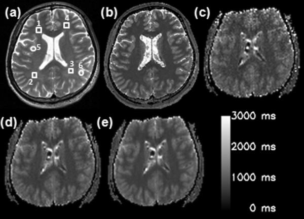
(a) T2–weighted image, and T1 maps using (b) IR-TSE and 2D ss-SESTEPI with signal averages of (c) 1, (d) 4, and (e) 16. ROIs are indicated by the square (white matter) and circles (gray matter). ROIs (1~4) and (5, 6) indicate white and gray matter, respectively
Table 1.
T1 relaxation time of gray and white matter at different regions of interest shown in Figure 7. 1 avg, 4 avg and 16 avg indicate multiple repetition average for SEPI and STEPI obtained by 2D ss-SESTEPI.
| Region | IR-TSE (ms) | 2D ss-SESTEPI (ms) | |||
|---|---|---|---|---|---|
| 1 avg | 4 avg | 16 avg | |||
| White matter |
1 | 722±33 | 799±58 | 721±41 | 728±20 |
| 2 | 716±26 | 727±68 | 726±30 | 722±20 | |
| 3 | 733±32 | 772±78 | 747±29 | 744±27 | |
| 4 | 685±33 | 742±89 | 725±40 | 715±27 | |
| Gray matter |
5 | 1276±90 | 1149±54 | 1101±61 | 1116±81 |
| 6 | 1177±90 | 1069±71 | 1087±80 | 1088±58 | |
In-vivo measurement of singleshot T1 in a mouse
Images in Fig. 8 are (a) T1 maps and (b) ΔR1 maps of selected time frames (every 30 sec.). T1 maps of 10 slices were obtained every 5 sec. Images in Fig. 8c are T1 weighted spin-echo images of pre-contrast and 10 min after contrast injection. Brightness indicates the larger values in T1 and ΔR1 maps. ΔR1 was plotted in Fig. 8c for several selected ROIs of 9 pixels and all at the 10 minute time point. Regions of 3×3 pixels (18 μL volume) were selected at kidney, tumor periphery, tumor core, and muscle. These data can be used for further pharmacokinetic evaluation pixel-by-pixel or by organ.
Figure 8.

Selected images of singleshot T1 mapping using 2D ss-SESTEPI in a tumor bearing nude mouse: (a) T1 maps, (b) ΔR1 map, (c) T1 weighted spin-echo images of various time points. The temporal resolution (TR) was 5 sec, with 1×1 mm2 resolution and 2 mm slice thickness. (d) Time curves of selected ROIs in (e) ΔR1 maps in a tumor bearing nude mouse. Numbered labels in the plots indicate the 9-pixel (18 μL) ROIs on ΔR1 maps; 1/kidney, 2/tumor periphery, 3/tumor core, and 4/noise.
DISCUSSION
B1 inhomogeneity correction was very successful with an experimentally measured correction map using the 2D ss-SESTEPI pulse sequence. Eq. 4, which describes the error in the T1 estimation using SEPI and STEPI without correction of B1 inhomogeneity, includes only the transmit function without signal reception. The measured B1 correction map, however, reflects all inhomogeneity causes including RF transmission and NMR signal reception, except for T1 and diffusion-weighted decays. The simulated plots in Fig. 2 agreed very well with the measured T1 in Fig. 4, which indicates that the correction method for B1 inhomogeneity is very robust. The only difference is a systematic underestimation. This probably results from diffusion-induced signal decay with the long diffusion time.
The accuracy of the resultant T1 value using 2D ss-SESTEPI decreased with a lower TM/T1 ratio, because there is not enough change in the T1 decay with a short TM, as shown in Fig. 5. Although the plots indicate that the measured T1 is more accurate with increased TM/T1, we have observed greatly decreased accuracy for very short T1 and large TM. This is because there was no signal left when TM is greater than 2~3 times T1. The choice of mixing time, therefore, depends on the spin-lattice relaxation time of interest. For instance, one may be interested in T1 < 1 s in DCE-MRI and T1 decreases with increased local concentration of MRI contrast agent. 0.4~0.5 s TM may be suitable for dynamic T1 mapping using paramagnetic-ion based contrast agents.
The T1 value was greatly underestimated for an increased spoiler area, as shown in Fig. 6. This diffusion-induced error in the T1 calculation is reduced by minimizing the zeroth moment A0 of the spoiler gradients. However, the minimum area of the spoiler gradient must be sufficient to spread the spin phase more than 2π within an imaging voxel, as in γA0.Δx > 2π for a smallest voxel dimension Δx. The b-factor was within the range of 10 ~ 30 s/mm2 for TM 0.4 s and 1~2 mm pixel dimension. For a typical diffusivity of 1.0×10⁻³ mm2/s in tissue water, the diffusion-weighted decay was 1~3 %, which may be ignored because it is within the noise level for STEPI images with SNR = ~ 30.
The important advantages of using 2D singleshot EPI are that the resultant images are free from motion-related artifact and have the highest signal-to-noise ratio (SNR) per fixed imaging time, which are crucial for quantitative MRI. However, 2D ss-EPI is very sensitive to the local variation of a non-linear background gradient caused by magnetic susceptibility at or near the tissue/air and tissue/bone interfaces, as in mouse images in Fig. 8. The resultant images suffer greatly from major geometric distortion that renders them useless. For singleshot EPI type acquisition, geometric distortion often becomes the largest limitation and its application is mostly restricted to diffusion and functional MRI of the intracranial brain, far from the sinus and the temporal bone. Therefore, it is crucial to reduce the susceptibility artifact in EPI images using 2D ss-SESTEPI before it may be useful for other applications. Because the degree of geometric distortion in 2D ss-EPI is proportional to the imaging field-of-view (FOV) in the phase-encoding direction, it can be reduced by using a reduced phase FOV. However, imaging a limited FOV in large surroundings induces aliasing in the phase-encoding direction in conventional MR imaging. The aliasing artifact can be completely removed while accomplishing interleaved multi-slice imaging by using double inversion/refocusing RF pulses with slice selection gradients applied perpendicular to the imaging RF pulses (19,22-24) or 2D spatially selective excitation (25).
Although the technique measures T1 in a singleshot in only a few seconds and the source images have low SNR, the resultant T1 was comparable to those measured using the inversion-recovery TSE. Average T1 values of GM and WM using 2D ss-SESTEPI and IR-TSE are summarized with other reported values (26-29) in Table 2. There is large variation among different reports, which may be because of different acquisition techniques. T1 in GM measured using 2D ss-SESTEPI was about 10 % lower than that using IR-TSE, while T1s in WM were similar to each other. This underestimation may result from the diffusion-induced signal decay in STE of SESTEPI. According to the literature (30), mean apparent diffusion coefficients (ADC) in posterior left white matter are 0.67×10⁻³ mm2 /s, while typical ADC in cortical gray matter are described as 1.0×10×3 mm2/s. Theoretical underestimation of T1 was calculated as 0.69 s and 1.169 s for GM and WM, respectively, using Eq. 4 with TM=0.6 s and b=23.8 s/mm2, assuming the true T1 values are 0.714 s (WM) and 1.226 s (GM) obtained using IR-TSE. These values are 3.0% and 4.6% different from T1s measured using IR-TSE.
Table 2.
Comparison of measured T1 values with previously reported values for gray and white matter in the brain at 3T.
As presented, rapid T1 mapping may be useful for non-invasive measurement of the concentration of the paramagnetic ion-based contrast agent. In our preliminary application of the technique for DCE-MRI on mice, the limiting factor for increased temporal resolution was signal-to-noise ratio. If a sufficient SNR is available by using a high-sensitivity RF coil or high-field MRI system, both temporal and spatial resolution can be improved.
CONCLUSIONS
2D ss-SESTEPI successfully measured both spin-echo and stimulated-echo in a singleshot. The magnitudes of both images are sensitive to the B1 variation within the imaging FOV, therefore correction for the B1 inhomogeneity is critical for T1 measurement. B1 inhomogeneity correction was successfully achieved by acquiring an additional stimulated-echo with minimal mixing time during the prescan, calculating the ratio between the spin-echo and the stimulated-echo and multiplying the stimulated-EPI by the inverse of the functional map. Realtime T1 measurement was possible using two images and an online image reconstruction program. It was possible to rapidly acquire T1 mapping in a few seconds, only limited by SNR of the source spin- and stimulated-EP images. The measured T1 agreed with those measured using conventional IR-TSE. 2D ss-SESTEPI may be an important tool for real-time in-vivo estimation of the concentration of paramagnetic-ion based contrast agent in DCE-MRI, because it is rapid and the resultant images are free-from motion-related artifacts.
ACKNOWLEDGEMENTS
This work was supported by the Benning Foundation, the Ben B. and Iris M. Margolis Foundation, a University of Utah VP Seed Grant, and NIH grants R21EB005705 and R01 EY015181. The authors thank Oliver Jeong for construction of the mouse coil and Dr. Yong-En Sun for mouse tail vein injections. The authors also are grateful to Dr. Roy Rowley for his help in proofreading the manuscript.
REFERENCES
- 1.Merboldt KD, Hanicke W, Bruhn H, Gyngell ML, Frahm J. Diffusion imaging of the human brain in vivo using high-speed STEAM MRI. Magn Reson Med. 1992;23(1):179–192. doi: 10.1002/mrm.1910230119. [DOI] [PubMed] [Google Scholar]
- 2.Farrell JA, Smith SA, Gordon-Lipkin EM, Reich DS, Calabresi PA, van Zijl PC. High b-value q-space diffusion-weighted MRI of the human cervical spinal cord in vivo: feasibility and application to multiple sclerosis. Magn Reson Med. 2008;59(5):1079–1089. doi: 10.1002/mrm.21563. [DOI] [PMC free article] [PubMed] [Google Scholar]
- 3.Aletras AH, Ding S, Balaban RS, Wen H. DENSE: displacement encoding with stimulated echoes in cardiac functional MRI. J Magn Reson. 1999;137(1):247–252. doi: 10.1006/jmre.1998.1676. [DOI] [PMC free article] [PubMed] [Google Scholar]
- 4.Frahm J, Bruhn H, Gyngell ML, Merboldt KD, Hanicke W, Sauter R. Localized high-resolution proton NMR spectroscopy using stimulated echoes: initial applications to human brain in vivo. Magn Reson Med. 1989;9(1):79–93. doi: 10.1002/mrm.1910090110. [DOI] [PubMed] [Google Scholar]
- 5.Slichter C. Principles of Magnetic Resonance. Springer-Verlag; Heidelberg: Germany: 1990. [Google Scholar]
- 6.Haacke E, Thompson M, Brown R. Magnetic Resonance Imaging, Physical Principles and Sequence Design. Wiley-Liss; 1999. [Google Scholar]
- 7.Haase A, Frahm J, Matthaei D, Hanicke W, Bomsdorf H, Kunz D, Tischler R. MR imaging using stimulated echoes (STEAM) Radiology. 1986;160(3):787–790. doi: 10.1148/radiology.160.3.3737918. [DOI] [PubMed] [Google Scholar]
- 8.Bornert Peter, Jensen Dye. Single-shot-double-echo EPI. Magn Reson Imaging. 1994;12(7):1033–1038. doi: 10.1016/0730-725x(94)91234-n. [DOI] [PubMed] [Google Scholar]
- 9.Feng Y, Jeong EK, Mohs AM, Emerson L, Lu ZR. Characterization of tumor angiogenesis with dynamic contrast-enhanced MRI and biodegradable macromolecular contrast agents in mice. Magn Reson Med. 2008;60(6):1347–1352. doi: 10.1002/mrm.21791. [DOI] [PMC free article] [PubMed] [Google Scholar]
- 10.Nicolle GM, Toth Eva, Schmitt-Willich Heribert, Raduchel Bernd, Merbach AE. The Impact of Rigidity and Water Exchange on the Relaxivity of Dendritic MRI Contrast Agent. Chem Eur J. 2002;8(5):9. doi: 10.1002/1521-3765(20020301)8:5<1040::aid-chem1040>3.0.co;2-d. [DOI] [PubMed] [Google Scholar]
- 11.Deoni SC, Rutt BK, Peters TM. Rapid combined T1 and T2 mapping using gradient recalled acquisition in the steady state. Magn Reson Med. 2003;49(3):515–526. doi: 10.1002/mrm.10407. [DOI] [PubMed] [Google Scholar]
- 12.Tofts PS, editor. Quantitative MRI of the Brain: measuring changes caused by disease. West Sussex, England: 2004. [Google Scholar]
- 13.Gowland P, Mansfield P. Accurate measurement of T1 in vivo in less than 3 seconds using echo-planar imaging. Magn Reson Med. 1993;30(3):351–354. doi: 10.1002/mrm.1910300312. [DOI] [PubMed] [Google Scholar]
- 14.Look DC, Locker DR. Time Saving in Measurement of NMR and EPR Relaxation Times. Review of Scientific Instruments. 1970;41(2):2. [Google Scholar]
- 15.Guo JY, Kim SE, Parker DL, Jeong EK, Zhang L, Roemer RB. Improved accuracy and consistency in T1 measurement of flowing blood by using inversion recovery GE-EPI. Medical physics. 2005;32(4):1083–1093. doi: 10.1118/1.1879732. [DOI] [PubMed] [Google Scholar]
- 16.Liu X, Feng Y, Lu ZR, Jeong EK. ISMRM. Berlin, Germany: 2007. Rapid Simultaneous Data acquisition of T1 and T2 Mapping, using Multishot EPI and Automated Variations of TR and TE at 3T; p. 1787. [DOI] [PMC free article] [PubMed] [Google Scholar]
- 17.Liu X, Feng Y, Lu ZR, Morrell G, Jeong EK. Rapid Simultaneous Acquisition of T1 and T2 Mapping Images using Multishot Double Spin-Echo EPI and Automated Variations of TR and TE (ms-DSEPI-T12) NMR Biomed. 2009 doi: 10.1002/nbm.1440. in print. [DOI] [PMC free article] [PubMed] [Google Scholar]
- 18.Norris DG. Implications of Bulk Motion for Diffusion-Weighted Imaging Experiments: Effects, Mechanisms, and Solutions. J Magn Reson Imag. 2001;13:486–495. doi: 10.1002/jmri.1072. [DOI] [PubMed] [Google Scholar]
- 19.Jeong EK, Kim SE, Kholmovski EG, Parker DL. High-resolution DTI of a localized volume using 3D single-shot diffusion-weighted STimulated echo-planar imaging (3D ss-DWSTEPI) Magn Reson Med. 2006;56(6):1173–1181. doi: 10.1002/mrm.21088. [DOI] [PubMed] [Google Scholar]
- 20.Liang ZP, Lauterbur PC. Principles of Magnetic Resonance Imaging: A Signal Processing Perspective. Wiley-IEEE Press; New York: 2000. [Google Scholar]
- 21.Wang Y, Ye F, Jeong EK, Sun Y, Parker DL, Lu ZR. Noninvasive visualization of pharmacokinetics, biodistribution and tumor targeting of poly[N-(2-hydroxypropyl)methacrylamide] in mice using contrast enhanced MRI. Pharmaceutical research. 2007;24(6):1208–1216. doi: 10.1007/s11095-007-9252-1. [DOI] [PubMed] [Google Scholar]
- 22.Feinberg DA, Turner R, Jakab PD. Echo-Planar Imaging with Asymmetric Gradient Modulation and Inner-Volume Excitation. Magn Reson Med. 1990;(13):162–169. doi: 10.1002/mrm.1910130116. [DOI] [PubMed] [Google Scholar]
- 23.Jeong EK, Kim SE, Guo J, Kholmovski EG, Parker DL. High-resolution DTI with 2D interleaved multislice reduced FOV single-shot diffusion-weighted EPI (2D ss-rFOV-DWEPI) Magn Reson Med. 2005;54(6):1575–1579. doi: 10.1002/mrm.20711. [DOI] [PubMed] [Google Scholar]
- 24.Feinberg D, Hoenninger J, Crooks L, Kaufman L, Watts J, Arakawa M. Inner volume MR imaging: technical concepts and their application. Radiology. 1985;156:743–747. doi: 10.1148/radiology.156.3.4023236. [DOI] [PubMed] [Google Scholar]
- 25.Saritas EU, Cunningham CH, Lee JH, Han ET, Nishimura DG. DWI of the spinal cord with reduced FOV single-shot EPI. Magn Reson Med. 2008;60(2):468–473. doi: 10.1002/mrm.21640. [DOI] [PubMed] [Google Scholar]
- 26.Wansapura JP, Holland SK, Dunn RS, RT, Ball WS. NMR Relaxation Times in the Human Brain at 3.0 Tesla. J Magn Reson Imaging. 1999;9:531–538. doi: 10.1002/(sici)1522-2586(199904)9:4<531::aid-jmri4>3.0.co;2-l. [DOI] [PubMed] [Google Scholar]
- 27.Stanisz GJ, Odrobina EE, Pun J, Escaravage M, Graham SJ, Bronskill MJ, Henkelman RM. T1, T2 Relaxation and Magnetization Transfer in Tissue at 3T. Magn Reson Med. 2005;54:507–512. doi: 10.1002/mrm.20605. [DOI] [PubMed] [Google Scholar]
- 28.Ethofer T, Mader I, Seeger U, Helms G, Erb M, Grodd W, Ludolph A, Klose U. Comparison of longitudinal metabolite relaxation times in different regions of human brain at 1.5 and 3 tesla. Magn Reson Med. 2003;50:1296–1301. doi: 10.1002/mrm.10640. [DOI] [PubMed] [Google Scholar]
- 29.Preibisch C, Deichmann R. T1 Mapping Using Spoiled FLASH-EPI Hybrid Sequences and Varying Flip Angle. Magn Reson Med. 2009;62:240–246. doi: 10.1002/mrm.21969. [DOI] [PubMed] [Google Scholar]
- 30.Chien Daisy, Buxton Richard B., Kwong Kenneth K., Brady Thomas J., Rosen BR. MR Diffusion Imaging of the Human Brain. Journal of Computer Assisted Tomography. 1990;14(4):514–520. doi: 10.1097/00004728-199007000-00003. [DOI] [PubMed] [Google Scholar]