Textural Kinetics: A Novel Dynamic Contrast-Enhanced (DCE)-MRI Feature for Breast Lesion Classification

Abstract

Dynamic contrast-enhanced (DCE)-magnetic resonance imaging (MRI) of the breast has emerged as an adjunct imaging tool to conventional X-ray mammography due to its high detection sensitivity. Despite the increasing use of breast DCE-MRI, specificity in distinguishing malignant from benign breast lesions is low, and interobserver variability in lesion classification is high. The novel contribution of this paper is in the definition of a new DCE-MRI descriptor that we call textural kinetics, which attempts to capture spatiotemporal changes in breast lesion texture in order to distinguish malignant from benign lesions. We qualitatively and quantitatively demonstrated on 41 breast DCE-MRI studies that textural kinetic features outperform signal intensity kinetics and lesion morphology features in distinguishing benign from malignant lesions. A probabilistic boosting tree (PBT) classifier in conjunction with textural kinetic descriptors yielded an accuracy of 90%, sensitivity of 95%, specificity of 82%, and an area under the curve (AUC) of 0.92. Graph embedding, used for qualitative visualization of a low-dimensional representation of the data, showed the best separation between benign and malignant lesions when using textural kinetic features. The PBT classifier results and trends were also corroborated via a support vector machine classifier which showed that textural kinetic features outperformed the morphological, static texture, and signal intensity kinetics descriptors. When textural kinetic attributes were combined with morphologic descriptors, the resulting PBT classifier yielded 89% accuracy, 99% sensitivity, 76% specificity, and an AUC of 0.91.

Introduction

Magnetic resonance imaging (MRI) is currently used as a complement to conventional X-ray mammography in diagnosis of breast lesions.¹ X-ray mammography remains the gold standard for breast cancer screening and offers high two-dimensional (2D) resolution, which is advantageous for detecting small variations in tissue composition, such as microcalcifications.² However, due to the constraints of imaging a three-dimensional (3D) structure in a single plane, ultrasound or breast dynamic contrast-enhanced (DCE)-MRI is often used as a secondary imaging technique when a suspicious lesion is found on mammography.² Ultrasound is very good at detecting tissue composition and hence is able to provide additional information to the mammogram in situations where the breast tissue is dense or a cystic mass needs to be ruled out.³ DCE-MRI is also very good at imaging dense breasts, but its major advantages over mammography and ultrasound are the ability to (a) image the entire breast as thin slices that comprise the entire breast volume and (b) measure variations in contrast uptake that provide information about the vascularity of the breast tissue. Since malignant tumors often have a high density of blood vessels that are poorly formed and thus leaky, they take up contrast dye at a different rate from benign lesions, allowing radiologists to distinguish malignant from benign lesions based on corresponding differences in contrast kinetics.^1,4

On account of breast DCE-MRI's high 3D resolution and its ability to acquire kinetic contrast information, its lesion detection sensitivity is close to 100%,⁵ much higher than that of either mammography or ultrasound.¹ However, specificity of breast DCE-MRI is low, with rates of between 30% and 70%^5,6 having been reported. High false positive detection rates on MRI often lead not only to anxiety for the patient but may also result in an unnecessary invasive biopsy.^1,5 In a review of the literature, Saslow et al.¹ found biopsy rates were between 3% and 15% when MRI was used for breast cancer screening in a high risk population, whereas the biopsy rates for mammography were 1–2%. In addition to the problem of low specificity, another shortcoming of breast MRI is that only experienced radiologists are able to accurately distinguish benign from malignant tumors.^1,7 This often leads to high rates of interobserver variability.⁷ Ikeda et al.⁷ reported this variability with kappa statistics between 0.21 and 0.40, where 1.0 represents complete agreement and 0.0 represents no agreement above the level expected by random chance. Therefore, one of the challenges in facilitating increased acceptance of breast DCE-MRI as a screening modality is reducing false positive detection errors, thereby boosting detection specificity. Additionally, the interobserver variability for breast DCE-MRI must be minimized.

To address the issues of low specificity and high interobserver variability in breast DCE-MRI, the American College of Radiology proposed the Breast Imaging Reporting and Data System (BIRADS),⁸ a semi-quantitative classification protocol for evaluating breast lesions. Lesions are evaluated on the basis of shape, margin morphology, internal enhancement, and kinetic or time–intensity curve characteristics.^9,10 Assuming that the imaging is complete, the radiologist gives each lesion seen on DCE-MRI a score between 1 and 6, where 1 is negative and 6 is known cancer⁸ based on the combination of lesion characteristics. Although the BIRADS system has helped to standardize the diagnosis of breast lesions, studies^1,7,9 continue to report significant variability in lesion interpretation among radiologists.

The remainder of this paper is organized as follows. In “Previous Work and Motivation,” we discuss the previous work in the analysis of breast DCE-MRI and computer-aided diagnosis (CAD) for breast DCE-MRI, as well as the motivation for the methods proposed in this paper. In “Materials and Methods,” we provide a description of the data and notational conventions employed and also describe our feature extraction schemes. We also provide details on the classifier methods used to quantify feature performance in “Materials and Methods.” In “Experiments and Performance Measures,” the experiments performed and the metrics used to evaluate the features are described. Quantitative and qualitative results showing the performance of the individual descriptors, as well as a combination of descriptors via two different classifiers, are presented in “Results.” Concluding remarks and future directions are presented in “Concluding Remarks.”

Previous Work and Motivation

In clinical decision-making, changes in signal intensity kinetics are an important descriptor for breast lesion characterization in DCE-MRI.^2,4,7,9–11 DCE-MRI involves first injecting a contrast agent such as gadolinium diethylenetriamine-pentaacid (Gd-DTPA) into the patient's bloodstream and concurrently acquiring a time series of MR images of the breast. Since malignant lesions tend to grow leaky blood vessels in abundance, the contrast agent is taken up by tumors preferentially.¹² Kuhl et al.⁴ found that data in the time series MRI could be plotted as single data points on a temporal curve, where the shape of the curve is reflective of the lesion class. It was shown⁴ that malignant lesions had a characteristic curve with a steep positive initial slope indicating rapid uptake of contrast agent and a subsequent negative slope indicating rapid washout. Benign lesions had slow contrast uptake (small positive initial slope) and then plateaued or did not reach peak intensity during the image acquisition period. Although signal intensity kinetics offer a great advantage to DCE-MRI for studying the functional attributes of breast lesions compared to other modalities, features derived from contrast enhancement data contribute to the high false positive rates reported for breast DCE-MRI.⁵ For instance, while both benign and malignant neoplastic tissue frequently have contrast enhancement patterns that differ from normal breast tissue, it is often difficult for radiologists to differentiate between benign and malignant lesions simply by visually inspecting the contrast-enhanced lesion on the postcontrast MRI. Consequently, several quantitative and semi-quantitative models have been proposed to measure the manner in which a lesion takes up the contrast dye.^11,13–28

Several computer-based image analysis systems have been proposed^{13–26,29,30} with the aim of reducing interobserver variability on breast DCE-MRI. CAD approaches for breast MRI are typically either for automatically (a) detecting a lesion (computer-aided detection (CADe))^{13–18,29,30} or (b) classifying a lesion as benign or malignant (computer-aided diagnosis (CADx)).^{13,15,19–26} Automated CADe approaches usually exploit the fact that malignant lesions typically have different signal intensity kinetic profiles on DCE-MRI compared to normal parenchyma.^{13–18,29,30} Some of these methods have been shown to have a detection accuracy comparable to manual detection.^{13–18,29,30} However, a CADx system assumes that the lesion detection has been solved either manually or via CADe, and it is typically comprised of two modules: (1) a quantitative feature extractor and (2) a classifier that employs the attributes extracted from the lesion to discriminate lesion classes. Several different CADx classifiers for DCE-MRI have been proposed including linear discriminant analysis (LDA),¹⁷ artificial neural networks,^6,15,19,20 and support vector machine (SVM) classifiers.²¹ Feature descriptors employed by CADx systems have typically included morphological,²⁰ lesion texture,^17,23 contrast enhancement,^13,15,21 or a combination of morphological and contrast enhancement descriptors.^6,19,22 Meinel et al.²⁰ found mean volume, area, radial length, spiculation, perimeter length, and compactness to be among the best morphological features, and their results with a back-propagation neural network classifier yielded an area under the curve (AUC) of 0.9748 on a dataset of 80 lesions using the leave-one-out method. Zheng et al.¹⁷ reported an AUC of 0.97 using temporal enhancement texture features on a cohort of 36 lesions. Gibbs et al.²³ reported an AUC of 0.80 using co-occurrence texture features on a cohort of 79 patients. However, by including patient data in the regression model, Gibbs et al.²³ achieved an accuracy of 92% and an AUC of 0.92. Using contrast enhancement alone, Chen et al.¹³ achieved an AUC of 0.85 over 121 studies, and Levman et al.²¹ obtained an AUC of 0.74 using empirical enhancement features such as signal enhancement ratio and time to peak enhancement over a cohort of 94 studies.

The three-time-point (3TP) model²⁴ and the pharmacokinetic (PK) model²⁷ are two common classifier-based approaches that focus on the kinetic contrast enhancement data and have been proposed for automated lesion diagnosis on DCE-MRI. The 3TP model developed by Degani et al.²⁴ assigns a color (red, green, or blue) to the slope of the contrast uptake portion of the kinetic curve and a color intensity between 0.0 and 1.0 to the contrast washout portion of the kinetic curve. The colormaps allow for a parametric visualization of the contrast enhancement profile by displaying each pixel as red if malignant, blue if benign, and green if suspicious for malignancy. Recently, on a dataset of 127 lesions,²⁶ the 3TP model yielded a sensitivity of 75.0% and a specificity of 83.1%, improving somewhat upon previously reported specificity results,^5,6 but sacrificing sensitivity. PK models differ from the 3TP method in that their objective is to provide a physiologic interpretation of the data by determining parameters such as K^trans (the transfer constant between the plasma and tissue compartments), υ_e (the extracellular extravascular volume fraction), and k_ep (the ratio of K^trans/υ_e).²⁷ Szabo et al.¹⁵ reported 71% sensitivity and 100% specificity using features derived from the Hayton PK model on a cohort of ten patients using a pixel-wise classifier. Veltman et al.³¹ reported an AUC of 0.83 with the Tofts PK model on a cohort of 102 lesions in 96 patients. While K^trans, υ_e, and k_ep have been shown to discriminate between lesion classes,²⁷ the computed values are highly sensitive to the choice of initial conditions.²⁸ Moreover, it has been noted in some recent studies^2,5,13 that the heterogeneity of lesion enhancement poses problems for the correct selection of pixels for the calculation of signal enhancement features.

The use of signal intensity kinetic profiles for lesion classification is also limited by other technical hurdles including MR artifacts such as bias field inhomogeneity³² and intensity nonlinearity.³³ An alternative to using temporal signal intensity profiles to characterize the lesion is to quantify the lesion texture, a somewhat nebulous term broadly used to refer to localized spatial variations in signal intensity. Lesion texture has also been acknowledged as an important lesion descriptor as evidenced by the incorporation of internal enhancement as a BIRADS descriptor for breast MRI lesion classification.⁸ While internal enhancement is intended for the assessment of the MRI at a single time point after contrast injection, it may also be useful to capture a measure of the change in this feature as a function of contrast enhancement. The concept of studying spatiotemporal textural patterns has been previously explored in Zheng et al.¹⁷ and Woods et al.¹⁸ Zheng et al.¹⁷ computed the discrete Fourier transform coefficients of kinetic changes in Gabor filter features to create parametric maps of the lesions. The authors reported an AUC of 0.97 using a leave-one-out LDA classifier on a cohort of 36 lesions. Woods et al.¹⁸ computed a four-dimensional co-occurrence matrix to calculate texture features in a pixel-wise fashion to differentiate between normal and malignant tissue. They were able to distinguish malignant and benign tissue areas with a sensitivity of 96.22% and a specificity of 99.85% on a dataset comprising four invasive ductal carcinomas and four benign lesions.

In this paper, a scheme is presented to analyze textural kinetic¹ curves, which quantify the spatiotemporal patterns of lesion texture during contrast uptake and diffusion. Instead of reducing the data into a single 2D image representation as in Zheng et al.¹⁷ and Woods et al.,¹⁸ the data here is presented in a manner familiar to radiologists and analogous to the signal intensity kinetic curves. Hence, the texture measures associated with the lesion at each pre- and postcontrast enhancement time point are plotted on a time series curve. Unlike previous studies,^17,18 the textural kinetic curves can be defined in multiple different parametric spaces (including Gabor, first-order statistical, and Haralick). Parameters obtained from model fitting these textural kinetic curves are employed in conjunction with a classifier to distinguish lesion classes. This allows for powerful multi-feature classifiers involving parameters from multiple textural and morphological representations to be easily constructed, unlike in previous studies,^17,18 which only consider spatiotemporal changes of certain attributes (Gabor¹⁷ and Haralick¹⁸). To illustrate the discriminability associated with the textural kinetic features, the signal intensity and corresponding textural kinetic curves for a second-order textural kinetic feature (contrast entropy) for ten benign (blue curves) and ten malignant lesions (red curves) are shown plotted in Figure 1(a) and (b), respectively. Each lesion was first manually segmented by an expert radiologist. The mean signal intensity, as well as the texture at each pre- and postcontrast time point, was calculated and then plotted. Figure 1(a) and (b) reveal that the textural kinetic feature was able to separate the benign from the malignant lesions better than signal intensity kinetics. The improved separation of lesion classes using the textural kinetic features appears to reinforce the fact that textural attributes may be more robust to bias field and intensity non-standardness³³ than image signal intensity.

Fig 1.

(a) Signal intensity and (b) a second-order textural kinetic curves (contrast entropy) for ten malignant (dotted red line) and ten benign (solid blue line) tumors over the course of contrast administration. Time = 0 is precontrast; progression along the normalized time axis denotes postcontrast time points. Time is normalized due to variability in the number of postcontrast time points among the datasets.

The main components of our methodology for assessing the performance of textural kinetic features as a lesion classifier on breast DCE-MRI are illustrated in the flowchart shown in Figure 2. Textural kinetic features are compared to signal intensity kinetic, morphologic, and pre- and peak contrast static texture descriptors of the lesion in distinguishing between benign and malignant breast lesions. The texture operators used include Gabor filters, first-order textural features, and second-order textural features. Gabor filters have been modeled on the patterning of the human visual cortex³⁴ and have found widespread application in image analysis.^17,33,34 First-order textural features (mean and median) give a global picture of lesion enhancement, whereas standard deviation and range yield insight into lesion heterogeneity. Second-order textural features, calculated via co-occurrence matrices,³⁵ reflect regional heterogeneity in the lesion. This may be particularly important, for example, in deciding if the malignant-type signal enhancement in a single pixel location in a lesion is an artifact or if there are neighboring pixels with similar signal intensities that corroborate the enhancement characteristics of a malignant lesion. Since both the SVM and probabilistic boosting tree (PBT) classifiers have been successfully employed for a variety of biomedical applications,³⁶ the classification performance of each feature is assessed with both an SVM classifier, which yields a hard benign or malignant classification, and a PBT classifier, which assigns a probability of malignancy to each lesion. In addition to the classifiers, graph embedding³⁷ is used to observe the clustering of the different lesions in a reduced-dimensional embedding space. After evaluating the individual features' performance, the features are combined to build a multi-feature classifier that aims to further improve lesion classification.

Fig 2.

Flowchart illustrating the steps comprising the methodology presented in this paper. Following manual lesion detection and segmentation, four different feature classes are extracted (morphological, signal intensity kinetics, precontrast texture, and peak contrast texture) to compare against textural kinetics. Quantitative evaluation of the five feature classes is done via support vector machine and probabilistic boosting tree classifier accuracy, while graph embedding is used for qualitative evaluation.

Materials and Methods

Data Description

A total of 41 (24 malignant and 17 benign) breast DCE-MRI studies were obtained from the Hospital at the University of Pennsylvania. All of these were clinical cases where a screening mammogram revealed a lesion suspicious for malignancy. All studies were collected under Institutional Review Board approval, and lesion diagnosis was confirmed by biopsy and histological examination. Sagittal T1-weighted, spoiled gradient echo sequences with fat suppression consisting of one series before contrast injection of Gd-DTPA (precontrast) and three to eight series after contrast injection (postcontrast) were acquired at either 1.5 Tesla or 3 Tesla (Siemens Magnetom or Trio, respectively). Single slice dimensions were 384 × 384, 512 × 512, or 896 × 896 pixels with a slice thickness of 3 mm. Temporal resolution between postcontrast acquisitions was a minimum of 90 s. The region of interest (ROI) associated with the lesion was then manually segmented via MRIcro imaging software³⁸ by an attending radiologist with expertise in MR mammography. The radiologist selected a 2D slice of the MRI volume that was most representative of each lesion, and the analyses were performed only for that 2D slice.

General Notation Used

We define a 2D section of a 3D MRI volume as  = (C,f^t), where C is a spatial grid of pixels c ∈ C, and f^t is the function that assigns a signal intensity value at every pixel c ∈ C and at each time point t ∈ {0, 1, 2,..., T − 1} in the DCE-MRI time series. t = 0 refers to the time at which the precontrast image is acquired, and t ∈ {1,..., T − 1} refers to the times at which the subsequent postcontrast images are acquired. The segmentation performed by the radiologist defines the boundary of the lesion, where the set of boundary points, , is a subset of the pixels contained in the lesion, , where  ⊂ C. The set of pixels in constitutes an eight-connected boundary such that for , , and , assuming unit spacing between the pixels in C. The coordinates of the centroid of are defined as , where , and || is the cardinality of set . Notation and symbols commonly used in this paper are shown in Table 1.

Table 1.

List of Notation and Symbols Commonly Used in This Paper

Symbol	Description	Symbol	Description
	2D MRI scene		Texture feature value for
C	2D grid of pixels,		Square neighborhood of length associated with each
	Spatial location of a pixel in C, where		Feature operator, where
	Set pixels corresponding to a lesion		Average feature value for operator over all
	A set of pixels defining the boundary of a lesion,		Classifier type
	Centroid of a lesion, defined by the 2D center of mass		Classifier output where
	Maximum radial distance of the lesion		Number of lesions identified as true positive, true negative, false positive, and false negative, respectively, using classifier
	A time point in the MRI time series,		Ground truth label of lesion,
	Signal intensity value associated with a pixel, , at time point,		Dataset comprised of lesions

Feature Extraction

Texture Features

A total of 92 precontrast texture features, 92 peak contrast texture features, and 92 textural kinetic features are calculated to describe the texture of each lesion in the dataset. After rescaling each image to a fixed grayscale intensity range, multiple different texture operators, , where represents the total number of features, are explored. The application of to each lesion yields a unique feature value, , associated with that lesion. The texture of the lesion before contrast agent injection (precontrast texture), the lesion texture at peak contrast enhancement, and the textural kinetic feature classes are obtained via application of several steerable, non-steerable, and statistical filters. Table 2 summarizes all texture features employed in this work.

Table 2.

Summary of All Textural Features Considered in This Paper with Associated Parameter Values

Texture feature class	Individual attributes	Parameters
Gabor filters	6 scales	,
	8 orientations
Kirsch filters	X-direction	Window size,
	Y-direction
	XY-diagonal
Sobel filters	X-direction	Window size,
	Y-direction
	XY-diagonal
	YX-diagonal
Gray level (first-order textural)	Mean	Window size,
	Median
	Standard deviation
	Range
	x-Gradient
	y-Gradient
	Magnitude of gradient
	Diagonal gradient
Haralick (second-order textural)	Contrast energy	Window size,
	Contrast inverse moment
	Contrast average	Maximum intensity,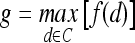
	Contrast variance
	Contrast entropy
	Intensity average
	Intensity variance
	Intensity entropy
	Entropy
	Energy
	Correlation
	Info. measure of correlation 1
	Info. measure of correlation 2

These features were used in the calculation of precontrast, peak contrast, and textural kinetics features

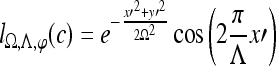
Gradient features Eleven non-steerable gradient features are obtained using Sobel and Kirsch edge filters and first-order spatial derivative operations. The Gabor filters, comprising the steerable class of gradient features, are defined by the convolution of a 2D Gaussian function with a cosine.³⁹ Hence, for every c ∈ , where ,^40,41 the Gabor filter bank response can be expressed as

1

where Λ is the wavelength of the sinusoid which controls the spatial frequency (scale) of the oscillations. The width of the Gaussian envelope Ω is used to define filters as a function of Λ such that Ω = 0.56Λ as derived in Kruizinga et al.³⁴ Filter orientation, φ, dictates the coordinate transformations: and . Six different scales and eight orientations are considered in constructing the Gabor filter bank.

First-order statistical features Four first-order statistical features (mean, median, standard deviation, and range) for three different square window sizes, s ∈ {3, 5, 7}, are calculated for the gray values of pixels within the sliding window . At every , and is the L₂ norm. Hence, average intensity, , within window is calculated as

2

where c ∈ C is the center pixel of the square window . Median, standard deviation, and range of image intensities within each for each c ∈ C are also calculated.

Second-order statistical features To calculate the second-order statistical (Haralick) feature scenes,³⁵ a pixel window, , s = 3, is defined. The parameter s = 3 is chosen to capture spatial variations at a high resolution because some of the smaller lesions in the dataset have an area just above 100 pixels. We then compute from each , c ∈ C, a g × g spatial gray level co-occurrence matrix G_c, where g is the maximum grayscale intensity of the image . The value at any location, , represents the frequency with which two distinct pixels, , with associated image intensities, , are adjacent (i.e., within the same 8-pixel neighborhood of ). A total of 13 second-order statistical³⁵ features (see Table 2) are extracted within each for every pixel for s = 3.

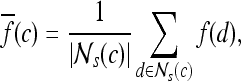
Textural Kinetic Features

For each , represents each of the different pixel-based pre- and postcontrast texture feature values, where and . The mean feature value, , within each lesion and at each time point t is then expressed as , and a corresponding textural kinetic vector, , is created. A third-order polynomial is fitted to to characterize its shape as

3

where are the model coefficients obtained by minimizing the root mean squared difference error between and , where and .

Signal Intensity Kinetic Feature

Signal intensity kinetic curves are calculated from the mean signal intensity within the lesion ROI in a manner similar to the curve generated and described in “Textural Kinetic Features.” The average lesion intensity is obtained as . The model coefficients of a third-order polynomial are obtained by the minimization procedure described in “Textural Kinetic Features.”

Morphological Features

For mass-like lesions, two important lesions descriptors in the BIRADS lexicon are lesion shape (e.g., round, oval, lobular, and irregular) and lesion margin (e.g., smooth, irregular, and spiculated).⁸ In this study, we consider six different quantitative descriptors modeled on the BIRADS attributes (Table 3 and Fig. 3).^42,43 The Area overlap ratio is a measure of lesion roundness, and the normalized average radial distance ratio, standard deviation of normalized distance ratio, variance of distance ratio, compactness, and smoothness are all descriptors for quantifying irregularity of the lesion boundary.

Table 3.

List of Morphological Features and Their Mathematical Descriptions

Morphological feature	Description
Area overlap ratio	where (see Fig. 3(a))
Normalized average radial distance ratio
Standard deviation of normalized distance ratio	,
	where and
Variance of distance ratio
Compactness	where ,
Smoothness	, where
	(see Fig. 3(b))

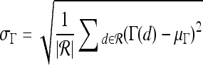
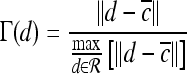
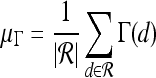
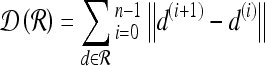
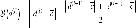
Fig 3.

Schematics illustrating the calculation of morphological features: (a) lesion boundary (red) and circle enclosing it (green) used to calculate area overlap ratio; (b) vectors used for calculation of lesion smoothness. is the lesion centroid, and are consecutive points on the lesion boundary.

Classification

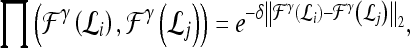
Support vector machine (SVM) The SVM classifier, , is employed to evaluate the ability of the lesion descriptors to discriminate between benign and malignant breast lesions on DCE-MRI. We construct by using a kernel function (∏) to project training data , where is the set of all lesions, onto a higher-dimensional space. This higher-dimensional space allows the SVM to construct a hyperplane to separate the two data classes (benign and malignant in our case). The is then evaluated by projecting testing data, , where into the same space and recording the location of the newly embedded datapoint with respect to the hyperplane. In our implementation, the radial basis function (RBF) kernel was employed to project the attributes with and , , where and , into a higher-dimensional space. The functional form of the RBF is given by⁴⁴

4

where δ is a scaling parameter. The general form of the SVM classifier is given as

5

where 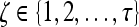represents the marginal training samples (i.e., support vectors), b is the hyperplane bias estimated for , and is the model parameter determined by maximizing an objective function subject to constraints which control the trade-off between empirical risk and model complexity.^45,46 represents the class labels, malignant and benign, respectively. represents the displacement from image to the hyperplane, and the output of the SVM classifier, , is equal to .

Probabilistic boosting tree (PBT) AdaBoost⁴⁷ is a popular ensemble machine-learning algorithm which yields a class label prediction by combining the outputs from several weak classifiers. However, in AdaBoost, the weighting scheme sometimes penalizes samples that are misclassified by a weak classifier even if they were previously correctly classified by a different weak classifier. Additionally, the order of features considered during classification is not preserved via Adaboost. The PBT algorithm⁴⁸ addresses these issues by iteratively generating a tree structure of length, B, in the training stage where each node of the tree is boosted with H weak classifiers. The hierarchical tree is obtained by dividing training samples, , into two subsets of and based on the learned strong classifier at each node using the standard AdaBoost algorithm⁴⁷ and recursively training the left and right subtrees. To avoid overfitting, the error parameter ϵ is introduced such that samples falling in the range are assigned to both subtrees with probabilities and , where the function represents the posterior class conditional probability of belonging to class +1 (malignant lesion). The algorithm stops when misclassification error hits a predefined threshold, θ. ϵ is set to 0.1 and as suggested in Tu.⁴⁸ During testing, the posterior class conditional probability of the sample being malignant is calculated at each node based on the learned hierarchical tree. The discriminative model is obtained at the top of the tree by combining the probabilities associated with probability propagation of the sample at various nodes. The output of the PBT classifier, , is defined such that if , then , else , where .For both the and , we use leave-one-out strategy for classifier training and evaluation. The training dataset, , is related to the test dataset, , by . During each iteration, contains only one lesion, one that was not considered as during previous iterations.

Three-time-point (3TP) modeling We compare our kinetic texture classifier to the popular 3TP classifier . The methods described in Degani et al., Weinstein et al., and Hauth et al.^24–26 are used to create a parametric map of signal intensity kinetics in the hue, saturation, and value (HSV) color space for each pixel in each lesion . Thus, the contrast washout rate is assigned to the hue channel, and the contrast uptake rate is assigned twice to both the saturation and value channels. Each pixel, , is assigned a red hue when representing highest likelihood of malignancy, green when representing moderate likelihood of malignancy, or blue when representing a low likelihood of malignancy. At each pixel, , 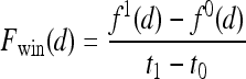and 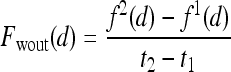, where is the precontrast time point, is the first postcontrast time point, and is the second postcontrast time point. and are rescaled between 0 and 1 for all . The empirical thresholds for the hue channel are as follows: if , then is assigned red (0 rad); if , then is assigned blue ; else if 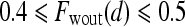then is assigned green . Both the saturation and value channels are set equal to the normalized value. A lesion is classified as malignant if it contains any red pixels and benign if it contains no red pixels .

Experiments and Performance Measures

Experiments

Discriminating Benign vs. Malignant Lesions Based on Individual Attributes from Morphological, Signal Intensity Kinetics, Precontrast Texture, Peak Contrast Texture, and Textural Kinetics Feature Classes

A total of 41 images (17 benign and 24 malignant) were analyzed. The separability of lesion classes (17 benign and 24 malignant) using individual descriptors from the feature classes (textural kinetic, precontrast texture, peak contrast texture, morphological, and signal intensity kinetics) was first qualitatively evaluated using graph embedding, a nonlinear dimensionality reduction technique.³⁷ We then compared the 283 individual descriptors to discriminate between benign and malignant lesions using two different quantitative classifiers, SVMs and PBTs. We also compare the SVM and PBT classification results to the 3TP classifier.

Discriminating Benign vs. Malignant Breast Lesions Based on a Combination of Features

Following identification of the top-performing features (“Discriminating Benign vs. Malignant Lesions Based on Individual Attributes from Morphological, Signal Intensity Kinetics, Precontrast Texture, Peak Contrast Texture, and Textural Kinetics Feature Classes”), all 283 individual attributes are combined in a pair-wise fashion to construct both a combined SVM and a combined PBT classifier. The performance of each combined multi-feature classifier (SVM and PBT) is then evaluated against individual attributes.

Performance Measures

Qualitative evaluation via graph embedding Graph embedding is a nonlinear dimensionality reduction scheme that is used to transform the high-dimensional set of image features into a low-dimensional embedding while preserving relative distances between images in the original feature space.^37,45 Given lesions and with corresponding feature vectors and , where and , an confusion matrix is constructed. The optimal embedding vector, X, is obtained from the maximization of the following function:

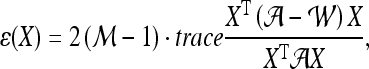6

where is the diagonal matrix where each diagonal element is defined as . The lower-dimensional embedding space is defined by the Eigenvectors corresponding to the smallest Eigenvalues of 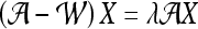. The matrix of the first Eigenvectors is constructed such that . In our case, so that the embedding basis vectors can be denoted, for any , where . Embedding plots of the data reduced to three dimensions were used to visualize each feature's ability to cluster the lesions into distinct categories.

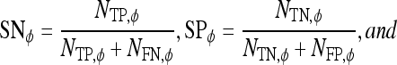
Quantitative evaluation For all three classifiers, , where , each lesion is identified as either a true positive (TP), false positive (FP), false negative (FN), or a true negative (TN) by comparing the classifier output, , to the true label, . If , lesion is identified as a TN; if , lesion is identified as a TP; if and , lesion is identified as an FP error; and if and , lesion is identified as an FN error. For each classifier, , the number of TP , TN , FP , and FN lesions over the entire set are calculated. Sensitivity , specificity , and accuracy for each classifier are then calculated as

7

8

where is the cardinality of set, E.

Receiver operator characteristic curves Receiver operating characteristic (ROC) curves representing the trade-off between sensitivity and specificity for breast cancer diagnosis were generated for both and . For _, a true ROC curve is generated since α, the probability decision threshold of the PBT, can be varied. Each point on the ROC curve corresponds to the sensitivity and 1-specificity over for some probability threshold , where the interval between α values, , is 0.05. In contrast to PBTs, SVM classifiers are typically used to generate a hard decision.⁴⁶ However, a pseudo-threshold can be generated for the SVM by converting the distance of each object to be classified from the SVM decision hyperplane into a soft likelihood of belonging to the object class. Thus, the greater the distance of the object from the hyperplane, the higher the likelihood that it belongs to a particular class; the proximity of an object to the hyperplane reflects higher ambiguity in the class assignment. The ROC curves for SVMs can be generated by varying the location of the decision hyperplane. As the distance of the objects from the decision hyperplane changes, the corresponding object-class probabilities also change. At each location of the decision hyperplane, classification sensitivity and specificity estimates are obtained. The trade-off between sensitivity and specificity obtained at each of the different locations of the hyperplane is used to generate an ROC curve.

Results

Qualitative Results

Figure 4 shows the embedding plots for the two features that separated the benign from malignant lesions best. The morphologic features and precontrast texture features did not clearly segregate the lesions, whereas the signal intensity kinetic feature and various textural kinetic features did indeed separate the data reasonably well into benign and malignant lesion categories. Although signal intensity kinetics produces a clustering of data classes that is similar to textural kinetic features (Figure 4(a)), the clusters appear better separated in the textural kinetic embedding space (Figure 4(b)).

Fig 4.

Embedding plots obtained by plotting the three dominant graph embedding vectors for (a) signal intensity kinetics and (b) gradient kinetics in the X-direction. Note that the increased separation of benign (blue) and malignant (red) lesions for the textural kinetics feature (b) compared to signal intensity kinetics (a).

Parametric maps Figure 5 shows representative images for two types of benign lesions and one type of malignant lesion. Each row shows the precontrast image (Fig. 5a, e, i), the postcontrast image corresponding to the peak lesion enhancement (maximum signal intensity across the time series) (Fig. 5b, f, j), the 3TP parametric map (Fig. 5c, g, k), and a parametric map for the textural kinetics feature for median, a first-order statistical feature (Fig. 5d, h, l). Note the differences in internal intensity in the textural kinetics maps (see Fig. 5d, h, l), especially between the malignant lesion and the two benign lesions. The malignant lesion in Figure 5(l) appears more heterogeneous in color than the two benign lesions, suggesting a higher heterogeneity in lesion enhancement patterns. In addition, the textural kinetic map of the malignant lesion in Figure 5(l) illustrates the difference between the enhancement pattern at the center of the lesion and at the periphery of the lesion.

Fig 5.

Examples of the contrast enhancement patterns associated with (a–d) a benign fibroadenoma, (e–h) a benign sclerosing adenosis, and (i–l) a malignant invasive ductal carcinoma. a, e, i Precontrast image. b, f, j Postcontrast image at peak enhancement. c, g, k 3TP maps corresponding to the studies in a, e, and i. d, h, l Textural kinetic maps for the median filter feature. The third and fourth columns are magnified to illustrate details of the lesion. Note that d, h, and l appear to capture heterogeneity of lesion enhancement (highest in l).

Quantitative Results

Classification of Lesions Using Individual Features with a Support Vector Machine Classifier

Table 4 shows that in conjunction with the SVM classifier, the best textural kinetic feature, contrast inverse moment, had greater values of accuracy than the best-performing morphology feature, smoothness, and signal intensity kinetics performed worse than smoothness. We also observed that textural kinetics of some of the Gabor filter features as well as some of the gray level features performed best in classifying the lesions. Note that when the was employed, the best-performing first-order (Gabor filters and median gray level) textural kinetic features also outperformed signal intensity kinetics in terms of accuracy, sensitivity, specificity, and AUC (Tables 4 and 5). These results are also reflected in the ROC curves shown in Figure 6, which correspond to the features shown in Table 5.

Table 4.

Results of Support Vector Machine Classifier for Top Five Performing Individual Features in Distinguishing Benign from Malignant Lesions Using Leave-One-Out Validation

Feature class	Feature
Morphological	Smoothness	0.73	0.88	0.53	0.77
First-order textural kinetics	Gabor filter	0.71	0.67	0.76	0.73
	Gabor filter	0.76	0.75	0.76	0.78
	Median gray level	0.76	0.75	0.76	0.78
Second-order textural kinetics	Contrast inverse moment	0.73	0.88	0.52	0.70

Table 5.

Results of Support Vector Machine Classifier for Top-Performing Individual Attributes from Each Feature Class in Distinguishing Benign from Malignant Lesions Using Leave-One-Out Validation

Feature class	Feature
Morphological	Smoothness	0.73	0.88	0.53	0.77
Precontrast texture	Gabor filter	0.63	0.90	0.25	0.65
Postcontrast texture	Intensity variance	0.68	0.83	0.47	0.70
Signal intensity	Signal intensity kinetics	0.63	0.67	0.59	0.75
First-order textural kinetics	Gabor filter	0.76	0.75	0.76	0.78
Second-order textural kinetics	Contrast inverse moment	0.73	0.88	0.52	0.70

Fig 6.

For the top-performing feature in each feature class, the receiver operating characteristic (ROC) curves for were generated by varying the distance of each lesion to be classified from the decision hyperplane. The individual features for which ROC curves have been plotted are second-order textural kinetic feature, contrast inverse moment; first-order textural kinetic feature, Gabor filter channel corresponding to ; morphology feature, smoothness; the Gabor filter channel corresponding to for the precontrast image; peak postcontrast texture, intensity variance; and kinetic signal intensity.

Classification of Lesions Using Individual Features with Probabilistic Boosting Trees

For , we found similar results to those obtained using . Using results from the operating point on the ROC curve (defined by the point on the curve that minimizes the Euclidean distance from the feature's ROC curve to the ideal 100% sensitivity, 100% specificity point on the graph) and the AUC, Tables 6 and 7 show that the kinetic second-order statistical feature, contrast inverse moment, performed the best from among both the top-performing features overall for (Table 6) and for each feature class (Table 7). The ROC curves in Figure 7 show that contrast inverse moment had the highest accuracy, sensitivity, and specificity at the operating point among the different feature classes.

Table 6.

Results of Probabilistic Boosting Tree Classifier for Top Five Performing Individual Features in Distinguishing Benign from Malignant Lesions Using Leave-One-Out Validation

Feature class	Feature
Morphological	Smoothness	0.85	0.91	0.76	0.91
First-order textural kinetics	Gabor filter	0.89	0.98	0.76	0.78
	Gabor filter	0.89	0.99	0.74	0.86
	Median gray level	0.90	0.97	0.81	0.83
Second-order textural kinetics	Contrast inverse moment	0.90	0.95	0.82	0.92

Table 7.

Results of Probabilistic Boosting Tree Classifier for Top-Performing Individual Attributes in Distinguishing Benign from Malignant Lesions Using Leave-One-Out Validation

Feature class	Feature
Morphological	Smoothness	0.85	0.91	0.76	0.91
Precontrast texture	Gabor filter	0.84	0.94	0.71	0.86
Postcontrast Texture	Intensity variance	0.70	0.92	0.41	0.58
Signal intensity	Signal Intensity kinetics	0.79	0.94	0.59	0.78
First-order textural kinetics	-gradient	0.83	0.88	0.76	0.85
Second-order textural kinetics	Contrast inverse moment	0.90	0.95	0.82	0.92

Note that the , , and values reported here are for the operating point on each feature's respective receiver operating characteristic curve. The operating point is defined as the point on the curve that minimizes the distance between the curve and the point (0,1), which corresponds to 100% sensitivity and 100% specificity on the graph

Fig 7.

Receiver operating characteristic (ROC) curves generated for by varying probability threshold, α ∈ [0, 1], for the top-performing feature in each feature class. ROC curves for second-order textural kinetic feature, contrast inverse moment; first-order textural kinetic feature, median gray level; morphology feature, smoothness; the Gabor filter channel corresponding to for the precontrast image; peak postcontrast texture, intensity variance, and kinetic signal intensity are shown.

Classification of Lesions Using 3TP Parametric Maps

The classification of all lesions in the dataset using the 3TP parametric maps produced an accuracy of 78%, sensitivity of 92%, and specificity of 59%.

Performance of Multi-feature Classifiers

We created multi-feature classifiers by combining each texture (pre-, peak contrast, and kinetic), kinetic signal intensity, and morphological feature in pair-wise combinations in conjunction with the SVM and PBT classifiers. The top-performing combination for both and are shown in Table 8. By combining smoothness and the textural kinetic feature for the Sobel filter oriented along the X-direction (X-direction Sobel filter) in conjunction with an SVM classifier , a classification accuracy of 82%, sensitivity of 85%, specificity of 71%, and an AUC of 0.78 using the leave-one-out strategy was obtained. By combining smoothness and the textural kinetic feature, contrast inverse moment kinetics, in conjunction with a PBT classifier , a classification accuracy of 89%, sensitivity of 99%, specificity of 76%, and an AUC = 0.91 using the leave-one-out strategy was obtained. In Figure 8, the embedding plot of the reduced feature space of a multi-feature classifier using graph embedding is shown. The embedding plot combining the textural kinetic feature X-gradient with the morphological feature, smoothness, appears to show good separation between the lesion classes and corroborates the performance of the multi-feature SVM and PBT classifiers.

Table 8.

Results of Classifiers Obtained by Combination of Multiple Attributes in Distinguishing Benign from Malignant Lesions Using Leave-One-Out Validation

Classifier combination
Smoothness + X-direction Sobel filter +	0.82	0.92	0.71	0.78
Smoothness + contrast inverse moment +	0.89	0.99	0.76	0.91

Fig 8.

Embedding plot obtained by plotting the three dominant graph embedding vectors for the combination of the morphology feature, smoothness, with the first-order textural kinetic feature, X-gradient. Note that the lesion classes appear to be better separated compared to Fig. 4.

Concluding Remarks

In this paper, we presented a new attribute, textural kinetics, for discriminating between benign and malignant lesions on breast DCE-MRI by quantifying the spatiotemporal patterns of lesion texture during the contrast enhancement time series. We showed that textural kinetic features outperformed the signal intensity kinetics feature on a dataset of 41 (17 benign and 24 malignant) breast lesions in terms of accuracy, sensitivity, and specificity. An SVM classifier in conjunction with the textural kinetic descriptors yielded an accuracy of 76%, sensitivity of 75%, specificity of 76%, and an AUC of 0.78, and the PBT classifier yielded accuracy of 90%, sensitivity of 95%, specificity of 82%, and AUC of 0.92. Textural kinetics appear to perform comparably to other texture-based approaches for lesion classification such as enhancement variance dynamics introduced by Chen et al.⁴⁹ and spatiotemporal enhancement profiles introduced in Zheng et al.¹⁷ Chen et al.⁴⁹ reported an AUC of 0.85 on a cohort of 121 datasets, whereas Zheng et al.¹⁷ reported an AUC of 0.97 on a cohort of 36 patients. Although textural kinetic features performed marginally worse than spatiotemporal enhancement profiles introduced in Zheng et al.,¹⁷ the study in Zheng et al.¹⁷ employed a smaller dataset (36 lesions), and the accuracy of their classifier decreased to less than 90% when the dataset decreased by five lesions, suggesting that the scheme might be sensitive to the composition of the dataset. The textural kinetic features yielded consistently good classification performance for both the SVM and PBT classifiers. When the textural kinetic attributes were combined with morphologic descriptors, the resulting SVM classifier yielded an 82% accuracy, sensitivity of 92%, specificity of 71%, and an AUC of 0.78, and the resulting PBT classifier yielded an 89% accuracy, sensitivity of 99%, specificity of 76%, and an AUC of 0.91, suggesting that pairing of morphology and signal intensity kinetic features with orthogonal lesion attributes such as textural kinetics could result in improved diagnosis of breast cancer on breast DCE-MRI. Previous studies^33,50 have suggested that textural attributes are likely more robust to MRI artifacts such as bias field and intensity non-standardness, which may explain the superior performance of our classifiers. The fact that textural kinetics appeared to outperform the classical BIRADS descriptors (albeit on a small cohort) suggests that this attribute should be considered when building a CAD system. It is important to note that what is presented here is not a full-fledged CAD system, but rather a study in the utility of textural kinetics in distinguishing benign from malignant lesions. In future work, we plan to more rigorously test the robustness of the features and combinations of features on a larger cohort. We also plan to incorporate automated lesion detection and segmentation into the current workflow.

References

- 1.Saslow D, Boetes C, Burke W, Harms S, Leach MO, Lehman CD, Morris E, Pisano E, Schnall M, Sener S, Smith RA, Warner E, Yaffe M, Andrews KS, Russell CA. American Cancer Society guidelines for breast screening with MRI as an adjunct to mammography. CA Cancer J Clin. 2007;57:75–89. doi: 10.3322/canjclin.57.2.75. [DOI] [PubMed] [Google Scholar]
- 2.Heywang-Kobrunner SH, Viehweg P, Hienig A, Kuchler C. Contrast-enhanced MRI of the breast: accuracy, value, controversies, solutions. Eur J Radiol. 1997;24:94–108. doi: 10.1016/S0720-048X(96)01142-4. [DOI] [PubMed] [Google Scholar]
- 3.Sickles EA, Filly RA, Callen PA. Benign breast lesions: ultrasound detection and diagnosis. Radiology. 1984;151:467–470. doi: 10.1148/radiology.151.2.6709920. [DOI] [PubMed] [Google Scholar]
- 4.Kuhl CK, Mielcareck P, Klaschik S, Leutner C, Wardelmann E, Gieske J, Schild HH. Dynamic breast MR imaging: are signal intensity time course data useful for differential diagnosis of enhancing lesions. Radiology. 1999;211:101–110. doi: 10.1148/radiology.211.1.r99ap38101. [DOI] [PubMed] [Google Scholar]
- 5.Piccoli CW. Contrast-enhanced breast MRI: factors affecting sensitivity and specificity. Eur Radiol. 1997;7(Suppl. 5):S281–S288. doi: 10.1007/PL00006909. [DOI] [PubMed] [Google Scholar]
- 6.Nie K, Chen J-H, Yu HJ, Chu Y, Nalcioglu O, Su M-Y. Quantitative analysis of lesion morphology and texture features for diagnostic prediction in breast MRI. Acad Radiol. 2008;15:1513–1525. doi: 10.1016/j.acra.2008.06.005. [DOI] [PMC free article] [PubMed] [Google Scholar]
- 7.Ikeda DM, Hylton N, Kinkel K, Hochman MG, Kuhl C, Kaiser WA, Weinreb JC, Smazal SF, Degani H, Viehweg P, Barclay J, Schnall MD. Development, standardization, and testing of a lexicon for reporting contrast-enhanced breast magnetic resonance imaging. J Magn Reson Imaging. 2001;13:889–895. doi: 10.1002/jmri.1127. [DOI] [PubMed] [Google Scholar]
- 8.Breast imaging reporting and data system atlas (BIRADS Atlas) Reston: American College of Radiology; 2003. [Google Scholar]
- 9.Kinkel K, Helbich TH, Esserman LJ, Barclay J, Schwerin E, Sickles EA, Hylton NM. Dynamic high-spatial-resolution MR imaging of suspicious breast lesion: diagnostic criteria and interobserver variability. AJR Am J Roentgenol. 2000;175(1):35–43. doi: 10.2214/ajr.175.1.1750035. [DOI] [PubMed] [Google Scholar]
- 10.Schnall MD, Blume J, Bleumke DA, DeAngelis GA, DeBruhl N, Harms S, Heywang-Kobrunner SH, Hylton N, Kuhl C, Pisano ED, Causer P, Schnitt SJ, Thickman D, Stelling CB, Weatherall PT, Lehman C, Gastonis CA. Diagnostic architectural and dynamic features at breast MR imaging: multicenter study. Radiology. 2006;238(1):42–53. doi: 10.1148/radiol.2381042117. [DOI] [PubMed] [Google Scholar]
- 11.Li K-L, Henry R, Wilmes LJ, Gibbs J, Zhu X, Lu Y, Hylton NM. Kinetic assessment of breast tumors using high spatial resolution signal enhancement ratio (SER) imaging. Magn Reson Med. 2007;58(3):572–581. doi: 10.1002/mrm.21361. [DOI] [PMC free article] [PubMed] [Google Scholar]
- 12.Kuhl C. MRI of breast tumors. Eur J Radiol. 2000;10:46–58. doi: 10.1007/s003300050006. [DOI] [PubMed] [Google Scholar]
- 13.Chen W, Giger ML, Bick U, Newstead GM. Automatic identification and classification of characteristic kinetic curves of breast lesion on DCE-MRI. Med Phys. 2006;33(8):2878–2887. doi: 10.1118/1.2210568. [DOI] [PubMed] [Google Scholar]
- 14.Stoutjesdijk MJ, Veltman J, Huisman H, Karssemeijer N, Barentsz JO, Blickman JG, Boetes C. Automated analysis of contrast enhancement in breast MRI lesions using mean shift clustering for ROI selection. J Magn Reson Imaging. 2007;26(3):606–614. doi: 10.1002/jmri.21026. [DOI] [PubMed] [Google Scholar]
- 15.Szabo BK, Aspelin P, Wiberg MK. Neural network approach to the segmentation and classification of dynamic magnetic resonance images of the breast: comparison with empiric and quantitative kinetic parameters. Acad Radiol. 2004;11:1344–1354. doi: 10.1016/j.acra.2004.09.006. [DOI] [PubMed] [Google Scholar]
- 16.Twellmann T, Meyer-Baese A, Lange O, Foo S, Nattkemper TW. Model-free visualization of suspicious lesions in breast MRI based on supervised and unsupervised learning. Eng Appl Artif Intell. 2008;21:129–140. doi: 10.1016/j.engappai.2007.04.005. [DOI] [PMC free article] [PubMed] [Google Scholar]
- 17.Zheng Y, Englander S, Baloch S, Zacharaki EI, Fan Y, Schnall MD, Shen D. STEP: spatiotemporal enhancement pattern for MR-based breast tumor diagnosis. Med Phys. 2009;37(7):3192–3204. doi: 10.1118/1.3151811. [DOI] [PMC free article] [PubMed] [Google Scholar]
- 18.Woods BJ, Clymer BD, Kurc T, Heverhagen JT, Stevens R, Orsdemir A, Bulan O, Knopp MV. Malignant-lesion segmentation using 4D co-occurrence texture analysis applied to dynamic contast-enhanced magnetic resonance breast image data. J Magn Reson Imaging. 2007;25:495–501. doi: 10.1002/jmri.20837. [DOI] [PubMed] [Google Scholar]
- 19.McLaren CE, Chen W-P, Nie K, Su M-Y. Prediction of malignant breast lesions from mri features: a comparison of artificial neural network and logistic regression techniques. Acad Radiol. 2009;16:842–851. doi: 10.1016/j.acra.2009.01.029. [DOI] [PMC free article] [PubMed] [Google Scholar]
- 20.Meinel LA, Stolpen AH, Berbaum KS, Fajardo LL, Reinhardt JM. Breast MRI lesion classification: improved performance of human readers with a backpropagation neural network computer-aided (CAD) system. J Magn Reson Imaging. 2007;25(1):89–95. doi: 10.1002/jmri.20794. [DOI] [PubMed] [Google Scholar]
- 21.Levman J, Leung T, Causer P, Plewes D, Martel AL. Classification of dynamic contast-enhanced magnetic resonance breast lesions by support vector mechines. IEEE Transact Med Imaging. 2008;27:688–696. doi: 10.1109/TMI.2008.916959. [DOI] [PMC free article] [PubMed] [Google Scholar]
- 22.Penn A, Thompson S, Brem R, Lehman C, Weatherall P, Schnall M, Newstead G, Conant E, Ascher S, Morris E, Pisano E. Morphologic blooming in breast MRI as a characterization of margin for discriminating benign from malignant lesions. Acad Radiol. 2006;13:1344–1354. doi: 10.1016/j.acra.2006.08.003. [DOI] [PMC free article] [PubMed] [Google Scholar]
- 23.Gibbs P, Turnbull LW. Texture analysis of contast-enhanced MR images of the breast. Magn Reson Med. 2003;50:92–98. doi: 10.1002/mrm.10496. [DOI] [PubMed] [Google Scholar]
- 24.Degani H, Gusis V, Weinstein D, Fields S, Strano S. Mapping pathophysiological features of breast tumors by MRI at high spatial resolution. Nat Med. 1997;3(7):780–782. doi: 10.1038/nm0797-780. [DOI] [PubMed] [Google Scholar]
- 25.Weinstein D, Strano S, Cohen P, Fields S, Gomori JM, Degani H. Breast fibroadenoma: mapping of pathophysiologic features with three-time-point, contrast-enhanced MR imaging—pilot study. Radiology. 1999;210(1):233–240. doi: 10.1148/radiology.210.1.r99ja18233. [DOI] [PubMed] [Google Scholar]
- 26.Hauth EAM, Jaeger H, Maderwald S, Muhler A, Kimmig R, Forsting M. Quantitative 2- and 3-dimensional analysis of pharmacokinetic model-derived variables for breast lesions in dynamic, contrast-enhanced MR mammography. Eur J Radiol. 2008;66(6):300–308. doi: 10.1016/j.ejrad.2007.05.026. [DOI] [PubMed] [Google Scholar]
- 27.Tofts PS, Berowitz B, Schnall MD. Quantitative analysis of dynamic Gd-DTPA enhancement in breast tumors using a permeability model. Magn Reson Med. 1995;33:564–568. doi: 10.1002/mrm.1910330416. [DOI] [PubMed] [Google Scholar]
- 28.Martel AL. A fast method of generating pharmacokinetic maps from dynamic contrast-enhanced images of the breast. Int Conf Med Image Comput Comput Assist Interv. 2006;9(Pt 2):101–108. doi: 10.1007/11866763_13. [DOI] [PubMed] [Google Scholar]
- 29.Vignati A, Giannini V, Bert A, Deluca M, Morra L, Persano D, Martincich L, Regge D: A fully automatic lesion detection method for DCE-MRI fat-suppressed breast images. Proceedings of SPIE Medical Imaging, 2009
- 30.Coto E, Grimm S, Bruckner S, Groller ME, Kanitsar A, Rodriguez O. MammoExplorer: an advanced CAD application for breast DCE-MRI. Proceedings of Vision, Modeling and Visualization, 2005
- 31.Veltman J, Stoutjesdijk M, Mann R, Huisman HJ, Barentsz JO, Blickman JG, Boetes C. Contrast-enhanced magnetic resonance imaging of the breast: the value of pharmacokinetic parameters derived from fast dynamic imaging during initial enhancement in classifying lesions. Eur Radiol. 2008;18(6):1123–1133. doi: 10.1007/s00330-008-0870-8. [DOI] [PMC free article] [PubMed] [Google Scholar]
- 32.Madabhushi A, Udupa JK, Souza A. Generalized scale: theory, algorithms, and application to image inhomogeneity. Comput Vis Image Underst. 2006;101(2):100–121. doi: 10.1016/j.cviu.2005.07.010. [DOI] [Google Scholar]
- 33.Madabhushi A, Feldman M, Metaxas DN, Tomaszewski J, Chute D. Automated detection of prostate adenocarcinoma from high-resolution ex vivo MRI. IEEE Transact Med Imaging. 2005;24(12):1611–1625. doi: 10.1109/TMI.2005.859208. [DOI] [PubMed] [Google Scholar]
- 34.Kruizinga P, Petkov N. Nonlinear operator for oriented texture. IEEE Transact Image Process. 1999;8(10):1395–1407. doi: 10.1109/83.791965. [DOI] [PubMed] [Google Scholar]
- 35.Haralick RM, Shanmugam K, Dinstein IH. Textural features for image classification. IEEE Transact Syst Man Cybernet. 1973;3(6):610–621. doi: 10.1109/TSMC.1973.4309314. [DOI] [Google Scholar]
- 36.Tiwari P, Rosen M, Madabhushi A. Dimensionality reduction scheme for detection of prostate cancer from magnetic resonance spectroscopy (MRS) Med Phys. 2009;36(9):3927–3939. doi: 10.1118/1.3180955. [DOI] [PMC free article] [PubMed] [Google Scholar]
- 37.Shi J, Malik J. Normalized cuts and image segmentation. IEEE Transact Pattern Anal Mach Intel. 2000;22(8):888–905. doi: 10.1109/34.868688. [DOI] [Google Scholar]
- 38.Rorden C, Brett M. Stereotaxic display of brain lesions. Behav Neurol. 2000;12(4):191–200. doi: 10.1155/2000/421719. [DOI] [PubMed] [Google Scholar]
- 39.Gabor D. Theory of communication. J Inst Elect Eng. 1946;93:429–457. [Google Scholar]
- 40.Grigorescu S, Petkov N, Kruizinga P. Comparison of texture features based on gabor filters. IEEE Transact Image Process. 2002;11:1160–1167. doi: 10.1109/TIP.2002.804262. [DOI] [PubMed] [Google Scholar]
- 41.Jain AK, Farrokhnia F: Unsupervised texture segmentation using Gabor filters. Proceedings IEEE International Conference on Systems, Man and Cybernetics, pp 14–19, 1990
- 42.Street WN, Wolberg WH, Mangasarian OL: Nuclear feature extraction for breast tumor diagnosis. IS&T/SPIE 1999 International Symposium on Electrical Imaging: Science and Technology, Vol. 1905, pp 861–70, 1993
- 43.Naik S, Doyle S, Feldman M, Tomaszewski J, Madabhushi A: Gland segmentation and computerized gleason grading of prostate histology by integrating low-, high-level and domain specific information. The Second International Workshop on Microscopic Image Analysis with Applications in Biology, 2007
- 44.Chapelle O, Haffner P, Vapnik V. Support vector machines for histogram-based image segmentation. IEEE Transact Neural Network. 1999;10:1055–1064. doi: 10.1109/72.788646. [DOI] [PubMed] [Google Scholar]
- 45.Lee G, Rodriguez C, Madabhushi A. Investigating the efficacy on nonlinear dimensionality reduction schemes in classifying gene and protein expression studies. IEEE/ACM Transact Comput Biol Bioinform. 2008;5:368–384. doi: 10.1109/TCBB.2008.36. [DOI] [PMC free article] [PubMed] [Google Scholar]
- 46.Cortes C, Vapnik V. Support-vector networks. Mach Learn. 1995;20(3):273–297. [Google Scholar]
- 47.Freund Y, Schapire RE. A decision-theoretic generalization of on-line learning and an application to boosting. J Comput Syst Sci. 1997;55:119–139. doi: 10.1006/jcss.1997.1504. [DOI] [Google Scholar]
- 48.Tu Z: Probabilistic boosting-tree: learning discriminative models for classification, recognition, and clustering. Proceedings of the Tenth IEEE International Conference on Computer Vision, Vol. 2, pp 1589–1596, 2005
- 49.Chen W, Giger M, Lan L, Bick U. Computerized interpretation of breast MRI: investigation of enhancement-variance dynamics. Med Phys. 2004;31:1076–1082. doi: 10.1118/1.1695652. [DOI] [PubMed] [Google Scholar]
- 50.Unay D, Ekin A, Cetin M, Jasinschi R, Ercil A: Robustness of local binary patterns in brain MR image analysis. Proceedings of the 29th Annual International Conference of the IEEE EMBS, 2098–2101, 2007 [DOI] [PubMed]