T₁ Mapping of the Gadolinium-Enhanced Myocardium: Adjustment for Factors Affecting Interpatient Comparison

Abstract

Quantitative T₁ mapping of delayed gadolinium-enhanced cardiac magnetic resonance imaging has shown promise in identifying diffuse myocardial fibrosis. Despite careful control of magnetic resonance imaging parameters, comparison of T₁ times between different patients may be problematic because of patient specific factors such as gadolinium dose, differing glomerular filtration rates, and patient specific delay times. In this work, a model driven approach to account for variations between patients to allow for comparison of T₁ data is provided. Kinetic model parameter values were derived from healthy volunteer time-contrast curves. Correction values for the factors described above were used to normalize T₁ values to a matched state. Examples of pre- and postcorrected values for a pool of normal subjects and in a patient cohort of type 1 diabetic patients shows tighter clustering and improved discrimination of disease state.

Myocardial delayed enhanced (MDE) cardiac magnetic resonance imaging (MRI) is a well-established technique used to evaluate ischemic (1–5) and nonischemic (6–9) disease of the myocardium. The method uses inversion recovery prepared T₁ weighted images obtained 5–30 min after administration of a gadolinium contrast agent. The inversion recovery pulse is set to null normal myocardium, while gadolinium concentration is greater in regions of focal myocardial scar, resulting in high signal intensity (10).

Qualitative evaluation of focal myocardial scar (i.e., from myocardial infarction) is a robust technique that appears to be relatively insensitive to variation in MDE MRI acquisition parameters (11). Gadolinium dose, however, is likely to influence the appearance of myocardial scar (12). On the other hand, diffuse myocardial fibrosis (i.e., from nonischemic cardiomyopathy) may show only minimal variation in signal intensity on MDE MRI, as a single voxel contains a mixture of both normal myocardium and abnormal myocardium. Indeed, in the theoretical case of complete, uniform dispersion of myocardial fibrosis, the inversion pulses used with the MDE technique will uniformly suppress the entire myocardium despite substantial retention of gadolinium. However, measured T₁ times are likely to be reduced in the presence of diffuse fibrosis/collagen, as recently demonstrated in some heart failure subjects (13).

Unfortunately, the observed T₁ time of the myocardium is affected by multiple parameters besides the extent of collagen deposition. For example, a longer time between the start of the gadolinium injection to the time of measurement of the T₁ map results in longer T₁ values due to renal excretion of gadolinium (14). Renal function and the extravascular volume of distribution of gadolinium may vary between patients. Iron deposition in certain diseases such as haemochromatosis will shorten T₁ times. Cardiac amyloidosis is associated with accumulation of amyloid protein and gadolinium retention. Although factors such as the timing of injection and imaging, as well as gadolinium dose are frequently under the control of the investigator, variation in physiologic parameters will confound the comparison of T₁ values between patients.

Thus, the observed T₁ time of the myocardium after gadolinium administration is a function of both physiologic parameters and MRI acquisition parameters. To derive inferences regarding tissue composition of the myocardium using the gadolinium technique, it is necessary to understand the influence of physiologic and acquisition parameters. In this study, we determined the sensitivity of MDE T₁ maps to both physiologic and MRI acquisition parameters, to correct for changes in these parameters between patients. We derived T₁ model parameters from MDE MRI studies on normal volunteers. As an example of how the methods may be applied, we then used these parameters to correct the observed T₁ values in a patient population at risk for diffuse myocardial fibrosis.

Methods

Model

To predict changes in T₁ with respect to contrast dose, time, glomerular filtrate rate (GFR), and hematocrit, one can use a multicompartment model for delayed enhancement similar to kinetic models used in PET (15). It is based on the assumption that the tissue can be simplified into compartments through which the passage of contrast agent can be modeled. A three compartment model is used, accounting for blood plasma, extracellular extravascular space (EES), and a trapping compartment to account for altered kinetics in scarred myocardium. Following the terminology from (15), the total tissue concentration is then given by

$$C_{\text{t}}(t)=V_{\text{p}}\cdot C_{\text{p}}+V_{\text{e}}\cdot C_{\text{e}}+V_{\text{trap}}\cdot C_{\text{trap}}$$ [1]

where V_p: volume of distribution of blood plasma, V_e: volume of distribution of EES compartment, V_trap: volume of distribution of trapping compartment

The blood plasma concentration curve has a biexponential form (16):

$$C_{\text{p}}(t)=D[a_{1}exp(-m_1\cdot t)+a_{2}exp(-m_2\cdot t)]$$ [2]

a₁, a₂, m₁, m₂ are constants. This form is valid only after first pass of the contrast agent for time, t >∼ 1 min. The first term is a fast exponent corresponding to equilibration between plasma and EES, whereas the second slow component corresponds to a disposition and elimination phase through glomerular filtration. D is the contrast dose in mmol/kg. Ideally, the arterial input function would be measured for each individual patient. However, this usually calls for a dedicated study as measurements at several time points over a long time duration are required. Such data are usually not obtained with MDE MRI. As a result, values determined in literature may provide an alternative.

For example, Tofts and Kermode (17) have used data from Weinmann (16) to derive the constants in Eq. 2. The values for a₁, a₂, m₁, and m₂ were found to be

$$\begin{array}{l}{a}_1=3.99\text{kg}/\text{L}\\ a_2=4.78\text{kg}/\text{L}\\ m_1=0.144/min\\ m_2=0.0111\end{array}$$ [3]

Once determined, they used the arterial input function so defined to study the time course of tracer concentration in lesions in the brain. Note that the analytic calculation of the amplitudes and decay constants is straightforward only under the condition that the plasma compartment is better connected to the extracellular space than to the kidneys. For a fixed dose per body weight, Weinmann found normal variation in the plasma concentration (arterial input function) to be between 10 and 15%.

Dependence on GFR

The dependence of the second exponential rate constant (m₂) on GFR was explored in (18) and can be expressed as

$$m_2=\text{GFR}/\text{ECFV}$$ [4]

where ECFV is the extracellular fluid volume. Equation 4 assumes that the filtered plasma volume per unit time is a constant and equal to GFR for substances such as Gd-DTPA that are completely filtered without tubular reabsorption or secretion. This is generally true if kidney function has not been compromised. The ECFV can be approximately calculated as (19):

$$\text{ECFV}=0.02154\times W^{0.6469}\times H^{0.7236}$$

where W is the weight in kg and H the height is in cm.

Substituting Eqs. 3 and 4 into 2 defines C_p(t) analytically in terms of dose, time, and GFR. Going back to the three compartment model (of Eq. 1), if one assumes that the perfusion effects are fast compared to those of delayed contrast enhancement, an analytical form can be found for C_t(t), the total tissue concentration, based on analytical forms for C_e(t) and C_trap(t).

$$C_{\text{e}}(t)=D(b_{1}exp(-m_1\cdot t)+b_{2}exp(-m_2\cdot t)+b_{3}exp(-K_2\cdot t))$$ [5]

where b₁=(K₂·a₁)/(K₂−m₁); b₂=(K₂·a₂)/(K₂−m₂); b₃=−(b₁+b₂) and K₂ is the rate constant between blood plasma and EES.

$$C_{\text{trap}}(t)=D(c_{1}exp(-m_1\cdot t)+c_{2}exp(-m_2\cdot t)+c_{3}exp(-K_2\cdot t)c_{4}exp(-K_4\cdot t))$$ [6]

where c₁=(K₄·b₁)/(K₄−m₁); c₂=(K₄·b₂)/(K₄−m₂); c₃=(K₄·b₃)/(K₄−K₂); c₄=−(c₁+c₂+c₃).

In Eq. 6, K₄ is the rate constant between EES and trapped component. Substituting [2], [4], [5], and [6] into [1] gives the total tissue concentration explicitly in terms of dose (D), time (t), and GFR:

$$C_{\text{t}}(t)=D\cdot [V_{\text{p}}\cdot \{a_{1}exp(-m_1\cdot t)+a_{2}exp(-(\text{GFR}/\text{ECFV})\cdot t)\}+V_{\text{e}}{b}_{1}exp(-m_1\cdot t)+b_{2}exp(-(\text{GFR}/\text{ECFV})\cdot t)+b_{3}exp(-K_2\cdot t)+V_{\text{trap}}\cdot \{c_{1}exp(-m_1\cdot t)+c_{2}exp(-(\text{GFR}/\text{ECFV})\cdot t)+c_{3}exp(-K_2\cdot t)+c_{4}exp(-K_4\cdot t)\}]$$ [7]

C_t(t) can, therefore, be explicitly determined if the gadolinium dose, time of acquisition, GFR, height and weight are known. Finally, the relationship between T₁ and total tissue contrast is through the relaxivity of the contrast agent:

$$1/T_1=1/T_{1\text{pre}}+r_1\cdot C_{\text{t}}(t)$$ [8]

where T_1pre is the T₁ in myocardium prior to contrast. In cases where T₁ prior to contrast is not available, T₁ ≈ 1070 ms (20) at 1.5 T can be assumed. r₁ is Gd relaxivity and is assumed to be 3.5 (mmol·s)⁻¹ at 1.5 T (21). Note that the relationship between gadolinium contrast dose and T₁ is linear only for T₁ > ∼ 260 ms at 1.5 T (18).

Correction for dose is obtained by fixing time = 15 min and m₂ = 0.0064 min⁻¹, while varying dose in small steps of 0.01 mmol/kg and calculating T₁ values using Eqs. 7 and 8 (after substituting for determined values of K₂ and V_e). The T₁ values so obtained are normalized by dividing the value of T₁ at dose = 0.15 mmol/kg by the T₁ values at other doses. This array is then used to correct for T₁ values obtained at a different dose by obtaining the multiplying factor corresponding to that dose from the array. Similarly, correction values are obtained for time and m₂ by varying the relevant parameter while holding the other two constant. The correction factors for dose, time, and m₂ are independent of each other and can be multiplied together to obtain the total correction factor.

A limitation of the above model is that first pass perfusion effects are not described. The above discussion also assumes that the rate of change of C_e(t) is primarily dependent on K₂, the volume transfer constant between EES and blood plasma. This is valid as contrast exchange between blood plasma and EES is fast compared with delayed contrast enhancement implying K₂ > K₄. A third assumption is that the rate constants are related to the volume transfer constants.

Gadolinium is mainly water soluble and binds only minimally to plasma proteins. The hematocrit will, therefore, affect the rate of exchange between blood plasma and the EES and consequently the total contrast in myocardium. This effect of hematocrit on tissue contrast can be ascertained by comparing the model from (18) with (22). One finds the following relationship between K₁ and hematocrit [Hct]:

$$K_1=K_{\text{i}}(1-[\text{Hct}])$$ [9]

where K_i is the unidirectional influx and [Hct] is expressed as a fraction of blood. Note that K₂ (Eq. 5 above) = K₁/V_e.

Experimental Studies

Normal Volunteer Studies

To determine values for various parameters in the kinetic model defined by Eq. 7, 13 healthy volunteers were scanned under IRB approved protocols on 1.5 T Avanto MRI scanners (Siemens, Erlangen, Germany). The volunteers had no history or symptoms of heart disease and were not on any medication. Informed consent was obtained for all study subjects. Single-slice T₁ determinations were performed at five time points (5, 10, 15, 20, and 25 min) using an inversion recovery True FISP Look Locker sequence in the four chamber view with the following scanning parameters: FOV = 380 × 297 − 326 mm, matrix size = 192 × 75 − 87, slice thickness = 8 mm, TR/TE = 2.5/1.1 msec, phase interval = 23–25 msec, flip angle = 50°, 22–46 phases acquired every other R-R interval (determined by heart rate). Gadolinium dose (Magnevist; Bayer Healthcare Pharmaceuticals, New Jersey, USA) was 0.15 mmol/kg (n = 6 subjects), 0.19 mmol/kg (n = 2 subjects), and 0.2 mmol/kg (n = 5 subjects). The parameters derived for the kinetic model should be invariant of the differences in dose. A precontrast scout scan was also performed to determine T₁ before contrast injection. Parameters for the precontrast scout scan were the same as the postcontrast scan parameters above. All volunteers had measurements of height, weight, and serum creatinine. Estimated GFR was determined from serum creatinine using the Modification of Diet in Renal Disease Study equation.

Patient Scans

Patients with type 1 diabetes from the Epidemiology of Diabetes Interventions and Complications (EDIC) study (23,24) underwent myocardial delayed enhancement MRI during the 14th follow-up year of the ongoing study. All patients were evaluated under investigational review board approved protocols and signed informed consent. Patients with type 1 diabetes are at substantially increased risk for premature cardiovascular disease. EDIC patients who were scanned on Siemens 1.5 T scanners using gadopentetate dimeglumine (Magnevist, Bayer Healthcare Pharmaceuticals, New Jersey, USA) as a contrast agent were considered for inclusion. We hypothesized that EDIC patients with more cardiovascular risk factors were more likely to have increased interstitial fibrosis and thus shorter postgadolinium myocardial T₁ time than patients with low cardiovascular risk. In addition, any systematic errors resulting from the use of different T₁ acquisition schemes could be discounted by doing a within the group comparison. Two patient groups were evaluated: (a) High-risk patients had hypertension (all were on antihypertensive medication or had blood pressure ≥140/90 mmHg), hyperlipidemia (all were on lipid lowering medication or had fasting serum low density lipoproteins>100 mg/dL), and poor glycemic control (HbA1c > 7%) (25). (b) EDIC patients with none of the above risk factors were assigned to the low-risk group. Twenty nine patients (19 high risk and 10 at low risk) from seven institutions met the inclusion criteria. Demographic characteristics and serum creatinine levels were available for all patients. T₁ values were computed from TI scout scans. The TI scout scan used a true FISP Look-Locker acquisition sequence in the four chamber (n = 21) or short axis (n = 8) view which was positioned at the mid-ventricle level. Parameters for the true FISP acquisition sequence were: TR/TE = 2.5/1.2 msec, flip angle = 50°, matrix size = 192 × 72, FOV = 360 × 290 mm, slice thick. = 8 mm, 30–45 phases with temporal resolution ≅ 25 ms. Gadolinium dose varied between 0.1 mmol/kg and 0.22 mmol/kg. The time from gadolinium injection to TI scout was extracted from the DICOM header. None of the patients exhibited focal myocardial scar.

Image Analysis

All images were processed off-line using MASS research software ((MASS V2010-EXP, Leiden University Medical Center, Leiden, The Netherlands). Left ventricular endocardial and epicardial borders were traced semiautomatically at all phases in each sequence by a single reader. Typical pixel by pixel fit was performed to a three parameter model (A − B_exp[−TI/T₁*]) to obtain T₁ (as T₁ = (B/A − 1)T₁*). The location of a pixel position within the myocardium can be described by its relative position across the local wall thickness (relative distance to the endocardial and epicardial contour) and its relative position along the length of the defined myocardial contours (from basal septal, to apex, to basal lateral). (For short-axis images the longitudinal location is defined by the angular position relative to the posterior junction of the RV free wall with the LV.) Following this definition, signal intensity curves of matching pixels were reconstructed and used for T₁ fitting. Prior to fitting, the signal intensity of initial phases was inverted. The best fit for T₁ value (corresponding to the smallest fitting error) was determined iteratively by inverting initial phases up to a time corresponding to the zero crossing of the longest possible T₁ value and performing a fit for each case. The Levenberg-Marquardt algorithm was used to perform a nonlinear fit of the three parameter model to the measured data. Only pixels where the χ² test for goodness of fit (26) was significant with level of significance α = 0.05 were included in the final average T₁ value. An example showing the myocardial wall contouring and mean T₁ fit is shown in Fig. 1. Figure 1c shows the mean measured values at each phase and the T₁ fit corresponding to the mean fit across the delineated myocardium.

FIG. 1.

Example of multiphase images obtained from a volunteer. a: Source images obtained using an inversion recovery True FISP Look Locker sequence in the four chamber view with FOV = 380 × 297 mm, matrix size = 192 × 75, slice thickness = 8 mm, TR/TE = 2.5/1.1 msec, phase interval = 23 msec, flip angle = 50°. b: Myocardial wall contouring. c: T₁ fitting over the entire myocardium.

The precontrast T₁ values showed a strong linear dependence on the heart rate, and a correction was applied to normalize values to a heart rate of 60 bpm. No statistically significant relationship was found between postcontrast T₁ values and heart rate. This is similar to findings in reference (27).

Results

Analysis of Normal Volunteer Data

Demographic and physiological parameters for the healthy volunteers are given in Table 1. A linear fit for precontrast T₁ values and heart rate was determined (Pearson correlation coefficient r = −0.89 (P < 0.01) and is shown in Fig. 2. Correction for heart rate was then applied based on the linear fit. Table 2 shows T₁ values obtained for the 13 volunteers before and after application of the correction factors. Mean T₁ value before correction was T₁ = 986.4 ± 168.1 msec, whereas after normalization to 60 bpm, it was 983.3 ± 84.5 msec. Decrease in the standard deviation of the mean values after correction suggests correction for variation of acquisition/physiologic variation between study subjects. Heart rate correction accounted for the major correction factor in study subjects prior to gadolinium contrast injection.

Table 1. Demographical and Physiological Parameter Variation for 13 Volunteers Used to Determine Kinetic Model Parameter Values.

	Normal volunteer studies (n = 13) Mean ± SD or Percentage (%)
Age (years)	38.1 ± 11.1
Gender, Male	54%
Weight (kg)	80.9 ± 18.0
Height (cm)	170.4 ± 8.1
BMI (kg/m2)	27.8 ± 5.5
Creatinine (mg/dL)	0.8 ± 0.3
GFR (mL/min/1.73 m2)	99.0 ± 32.7

FIG. 2.

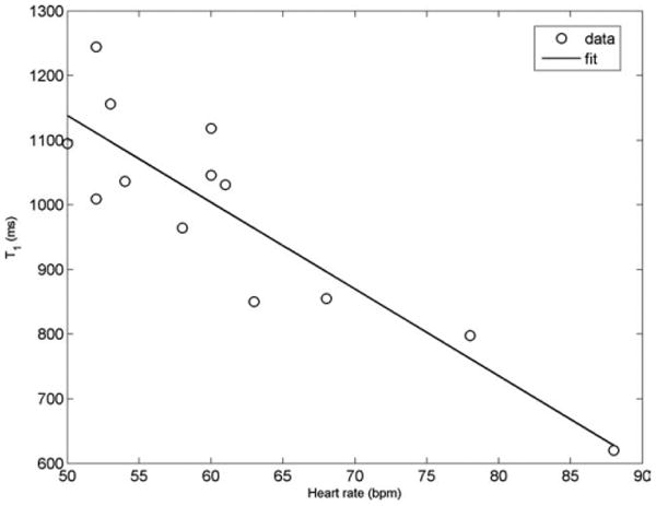
Precontrast T₁ values of the myocardium showed a strong negative linear correlation to heart rate (Pearson r = −0.89).

Table 2. Precontrast T₁ Values for 13 Normal Volunteers Before and After Correction for Variation in Heart Rate.

Study subject number	T1 (precontrast) (msec)	Heart rate (bpm)	T1 (precontrast), corrected (ms)
1	1036	54	953
2	1031	61	1045
3	1118	60	1118
4	620	88	853
5	1244	52	1111
6	850	63	885
7	1156	53	1048
8	1046	60	1046
9	855	68	946
10	964	58	939
11	1095	50	948
12	1009	52	901
13	798	78	990
mean ± standard deviation	986 ± 168	60a	983 ± 84

^aNormalized to heart rate of 60 bpm.

Postcontrast T₁ vs. time data were fit to Eq. 7 after determining C_t from Eq. 8. A multiparameter fit using Nelder-Mead unconstrained nonlinear minimization (Matlab^®) provided values for K₂ and K₄. Values for b₁, b₂, b₃, c₁, c₂, c₃, and c₄ were subsequently determined, and the set of Eqs. 5–7 were solved for V_e and V_trap after assuming V_p = 0.08 (18,22). The least squares fit resulted in values for V_trap that were close to 0 or negative. This indicated that the V_trap component was negligible. As a result, the trapping compartment was discarded by setting K₄ = 0 and performing the above process assuming the absence of a trapping component. Table 3 shows the T₁ values at the five time points and the corresponding values for the parameters (K₂ and V_e) derived from the resulting kinetic model. Mean and standard deviation values for K₂ and V_e were determined to be 8.05 ± 1.65 min⁻¹ and 0.26 ± 0.06. (These values are similar to the values reported in (15) where K₂ = 7.3 min⁻¹ and V_e = 0.30 for noninfarcted myocardium.)

Table 3. Measured T₁ Values (in msec) at time = 5, 10, 15, 20, and 25 min and the Corresponding Kinetic Model Values (K₂, V_e) for Normal Volunteers.

Study subject number	Delay time: t = 5min	10 min	15 min	20 min	25 min	Average T1 (precorrection) mean ± std	Average T1 (postcorrection) mean ± std	K2 (min−1)	Ve
1	420.1	499.4	535.5	552.2	581.2	517.7 ± 62.1	520.7±21	8.895	0.2715
2	379.8	457.1	513.0	552.7	572.5	497.4 ± 78.4	477.4 ± 29.4	10.151	0.3801
3	463.0	538.2	564.5	603.6	620.4	557.9 ± 62.1	569.7 ± 13.6	6.528	0.2645
4	346.8	421.0	441.4	465.4	509.8	494.4 ± 66.1	501.7 ± 29.3	6.583	0.2565
5	408.2	492.2	538.3	581.0	619.1	527.7 ± 81.9	524.2 ± 35.8	8.327	0.3307
6	374.9	420.0	459.0	462.0	491.1	441.4 ± 45	505.3 ± 12.8	8.32	0.2572
7	445.2	492.8	500.3	567.6	561.3	513.4 ± 51.2	596.6 ± 18.6	6.934	0.2125
8	356.2	415.4	442.2	451.2	473.9	427.8 ± 45.2	517 ± 10.4	9.284	0.3052
9	399.2	491.2	513.5	490.6	533.3	485.5 ± 51.4	492.7 ± 24.1	8.971	0.3077
10	413.1	456.3	500.0	549.4	530.8	489.9 ± 55.5	579.8 ± 22.5	11.088	0.1962
11	365.3	432.5	449.9	474	500.47	444.4 ± 51.1	528.5 ± 19.2	7.744	0.2551
12	412.42	460.25	507.6	531.4	537.5	489.8 ± 52.9	572.6 ± 16.7	6.42	0.1882
13	418	473.42	488.4	567.8	520.4	493.6 ± 55.6	583.5 ± 29.2	5.349	0.2089
Mean T1 ± mean s.d. across all volunteers:						491 ± 58	537 ± 22

Because the factors influencing T₁ are independent of each other, correction curves can be determined individually and multiplied together to determine T₁ value at a fixed (dose, time, GFR) value. Note that m₂ ∝ GFR and can be used instead of GFR. Figures 3–5 show corrections for dose, time, and m₂ where normalization is done corresponding to dose = 0.15 mmol/kg, time = 15 min, and m₂ = 0.0064 min⁻¹ (corresponding to GFR = 90 mL/min/1.73 m² for weight = 70 kg and height = 175 cm). Figure 6 shows correction values when [Hct] is varied from 0.3 to 0.5 for different acquisition times. For time points of typical interest (>5 min), differences in [Hct] have negligible impact on T₁ values and can be ignored.

FIG. 3.

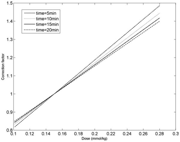
Correction curves for changing dose (dose = 0.1 to 0.28 mmol/kg) and for different delay times after the injection of gadolinium. The correction factor on the y-axis is in reference to a gadolinium dose of 0.15 mmol/kg.

FIG. 5.

Correction for varying GFR at different time values. The correction factor on the y-axis is in reference to m₂ = 0.0064 min⁻¹ (corresponding to GFR = 90 mL/min/1.73 m² for weight = 70 kg and height =175 cm).

FIG. 6.

Correction for hematocrit fraction variation for different time values. The correction factor on the y-axis is in reference to a hematocrit level of 0.40.

T₁ values obtained in the 13 volunteers at each of the 5 time points (Table 3) were normalized to the above three values for dose, time, and m₂. The mean and standard deviations across all time points and volunteers before and after correction for variation in dose, time, and GFR are shown in Table 3. Prior to normalization, the mean T₁ was 491 ± 58 msec. After normalization, the mean T₁ was slightly longer (T₁ = 537 msec). The corrected T₁ time lengthened as expected since the average administered gadolinium dose (0.175 mmol/kg) was greater than the normalized dose of 0.15 mmol/kg. As expected, the standard deviation of the mean T₁ time for each volunteer also decreased (average, 58 msec to 22 msec) after the correction factor was applied for each delay time from 5 to 25 min.

Analysis of Diabetic (EDIC) Patient Data

Characteristics of the patients with type 1 diabetes are presented in Table 4. None of the patients had focal myocardial scar. Patients at seven different institutions meeting the inclusion criteria had MRI scans obtained. Despite central standardization of the MRI protocol, institutional requirements and technologist variation resulted in wide variation of scanning parameters. The gadolinium dose varied between 0.1 mmol/kg and 0.22 mmol/kg. The time at which the Look-Locker sequence was obtained varied from 8 to 16 min after the start of the gadolinium injection. The estimated glomerular filtration rate varied between 64.8 and 114.1 mL/min/1.73 m². Thus, uncorrected T₁ values of the myocardium would not be likely to reflect differences in the intrinsic myocardial tissue. Instead, T₁ differences between patients were likely to be confounded by differences in both physiologic and scan acquisition parameters.

Table 4. Demographical and Physiological Parameters for Patients with type 1 Diabetes Categorized at Low and High Risk^a for Cardiovascular Disease (CVD).

	Patients with high CVD risk (n = 19) Mean ± SD or Percentage (%)	Patients with low CVD risk (n = 10) Mean ± SD or Percentage (%)
Age (years)	50.3 ± 5.0	48.1 ± 7.0
Gender, Male	58%	80%
Weight (kg)	87.6 ± 16.8	79.9 ± 8.9
Height (cm)	172.3 ± 9.1	175.1 ± 7.7
BMI (kg/m2)	29.3 ± 3.5	26.0 ± 2.4
Creatinine (mg/dL)	0.9 ± 0.1	0.9 ± 0.1
GFR (mL/min/1.73 m2)	81.5 ± 13.3	89.5 ± 14.2

^aHigh-risk patients had hypertension (all were on anti-hypertensive medication or had blood pressure ≥140/90 mmHg), hyperlipidemia (all were on lipid lowering medication or had fasting serum low density lipoproteins >100 mg/dL), and poor glycemic control (HbA1c > 7%). Low-risk patients had none of these risk factors and had HbA1c≤ 7%.

Before normalization, the mean T₁ values for the low-risk and high-risk patients were 479 ± 50 msec and 450 ± 48 msec, respectively (P ≅ 0.13, Students t-test). If fibrosis were present due to cardiovascular risk factors, we would have expected the high risk group to have reduced mean T₁ values than the low risk group. After normalization, mean T₁ values for the low-risk and high-risk patients were 548 ± 59 ms and 499 ± 59 ms, respectively (P < 0.05, Students t-test) (Fig. 7). The results suggest that greater cardiovascular risk in type 1 diabetes patients is associated with shorter T₁ time after gadolinium administration. Note that the etiology of the difference in T₁ times between groups is not determined by this methodology.

FIG. 7.

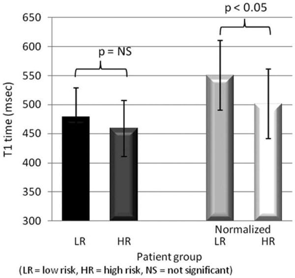
T₁ values for low- and high-cardiovascular risk diabetic patients before and after normalization. (*p < 0.05 for difference after normalization). Before normalization, gadolinium dose ranged from 0.1 mmol/kg to 0.22 mmol/kg, delay time from 8 to 16 min, and GFR from 64.8 to 114.1 mL/min/1.73 m². Data were normalized to a dose of 0.15 mmol/kg, delay time of 15 min, and m₂ = 0.0064 min⁻¹ (GFR = 90 mL/min/1.73 m² for weight = 70 kg and height = 175 cm).

Discussion

We have described a kinetic model based correction for T₁ values obtained with varying physiological and scanning parameters. Values for the kinetic model were derived using T₁ mapping data obtained at five different time points from normal volunteers. The applicability of the correction based on values determined from healthy volunteer time-contrast data should be valid in studies where subjects or patients exhibit nonscarred myocardium. In patients with heart failure and diffuse interstitial fibrosis, renal function is frequently diminished so that GFR corrections will be especially needed.

We applied these results to a patient group at high risk for cardiovascular disease. Patients with type 1 diabetes in the EDIC study have a significantly increased likelihood of developing cardiovascular disease. None of the patients considered here had scarred myocardium. Because fibrosis is not visible using MDE MRI, we included the entire myocardium for T1 measurements. Care was taken to avoid partial volume effects by excluding voxels at the edge of the myocardium. After correction values were applied, EDIC patients with high cardiovascular risk showed shorter T₁ values compared to low-risk patients. Although only postcontrast T₁ values were studied for this patient population, it is also possible that precontrast values may vary between the high- and low-risk groups (see also discussion below). The EDIC study is an observational cohort, so that biopsies were not obtained. Nevertheless, this patient population was useful to demonstrate the potential role of the correction factor approach for comparing T₁ values between study subjects. Further effort as to the etiology of T₁ differences between the groups remains to be performed.

The majority of variation in T₁ time was due to gadolinium dose, followed by MRI scan delay time after gadolinium injection and the patient's glomerular filtration rate (Figs. 3–5). Even if gadolinium dose and delay time could be standardized, it is well recognized that renal failure is highly associated with cardiovascular disease events (28,29). Heart rate for single R-R interval acquisitions has a negative correlation with precontrast T₁ values. A linear relationship between heart rate and uncorrected T₁ was assumed. It is possible that the relationship is nonlinear. A theoretical treatment of the relationship would require considerable effort and is outside the purview of this study. Although postcontrast T₁ values did not show a statistically significant relationship with heart rate (r = 0.45 to 0.6), correction for heart rate may be useful at elevated heart rates. The heart rate for two of the normal volunteers was higher (78 bpm and 88 bpm) during the T₁ scout scan but maintained sinus rhythm. We attributed the elevated rates to volunteer discomfort or anxiety during scanning. Precontrast T₁ of myocardium is about two times the postcontrast value. The allowed recovery time (two R-R intervals) is then insufficient to restore magnetization to its equilibrium value before the next inversion pulse. On the other hand, most of the magnetization has recovered to the equilibrium value for the case of postcontrast myocardium. This is similar to findings in (27), although the acquisition schemes are not identical. The True FISP sequence used with scout scans could be sensitive to B₀ inhomogeneities. However, with a short TR as used here and at 1.5 T, B₀ variation was not a factor. In addition, B₁ variation is also not a factor with inversion recovery LL as used here, as it gets reflected in the other parameters used to fit the measured data to the model. The final kinetic model revealed the lack of a trapping component. This can be partially explained by the differences in the values of c₁, c₂, c₃, and c₄ which are consistent with derivation of b₁, b₂, and b₃ and, therefore, differ from the values reported in (15). Hematocrit variation was found to have a negligible effect on T₁ correction (Fig. 6).

With the increase in the number of multicenter studies using cardiac MRI, data mining to explore patterns and discover associations retrospectively is gaining in importance. Such studies, often involving hundreds or thousands of subjects, such as EDIC (23,24) or MESA (Multiethnic study of atherosclerosis) (30,31), provide potentially invaluable data regarding myocardial function and structure. However, large studies may have substantial variation in institution specific requirements for gadolinium contrast agent administration in the era of nephrogenic systemic fibrosis. Under such circumstances, a normalization scheme such as the one presented here could be valuable. This preliminary work suggests that the likelihood of discrimination between high-risk and low-risk diabetic patients improves after T₁ normalization. Our conclusions are also supported by results for the normal volunteer studies where variations due to delay times were reduced upon normalization.

There are multiple limitations of this analysis. The kinetic model derivation makes several assumptions regarding the various compartments and characteristics of the contrast agent. In addition, the correction factors derived show a strong relationship to the assumed value of contrast agent relaxivity. By using a different relaxivity for Magnevist (4.1(mmol·s)⁻¹ (32) instead of 3.5(mmol·s)⁻¹), only different values for kinetic parameters K₂ (6.94 min⁻¹ instead of 8.05 min⁻¹) and V_e (0.24 instead of 0.26) result, but these did not alter the corrected T₁ values in any appreciable manner. The reported relaxivity values for different gadolinium contrast agents vary (from 4.1 (mmol·s)⁻¹ for Magnevist to 6.3 (mmol·s)⁻¹ for Multihance (Bracco Diagnostics Inc, New Jersey, USA (32)), so that standardization of gadolinium type is likely to be helpful when comparing T₁ times between patients. Also, in this study, we have focused on T₁ shortening due to gadolinium contrast agent. However, myocardial iron deposition may also cause T₁ shortening, and the derived models do not account for this parameter. The etiology of the differences in T₁ times for the low- and high-risk diabetic patients is not known as biopsies could not ethically be obtained. In that case, we reasoned that the low-risk group was likely to be a better control group than an external group of normal volunteers. We caution that the T₁ values we present for the normal volunteers were suitable for proof of concept of the normalization approach, but a larger, better clinically and biochemically characterized control group would be helpful to determine “normal” T₁ values of the myocardium. Note that multiple correction factors will increase the uncertainty (standard deviation) of the normalized T₁ values. In addition, the arterial input function shows some variation between volunteers or patients. Thus, the correction technique may not detect subtle differences in T₁ times between individual study subjects. Efforts to improve the accuracy and reproducibility of T₁ measurement of the myocardium via better pulse sequences (33), as well as standardization of the MRI scan protocol and gadolinium dose will reduce errors in the normalized T₁ data.

In conclusion, T₁ determination of the myocardium is playing an increasing role in the assessment of tissue composition. The current methods are highly dependent on acquisition and patient parameters. The methods we have described appear useful to normalize the acquired data so that interpatient differences may be assessed. The T₁ correction tool can be accessed at http://www.cc.nih.gov/researchers/resources.shtml.

FIG. 4.

Correction curves for varying time and as a function of different doses of gadolinium. The correction factor on the y-axis is in reference to a standardized delay time of 15 min after gadolinium injection.

References

- 1.Kim RJ, Chen EL, Lima JA, Judd RM. Myocardial Gd-DTPA kinetics determine MRI contrast enhancement and reflect the extent and severity of myocardial injury after acute reperfused infarction. Circulation. 1996;94:3318–3326. doi: 10.1161/01.cir.94.12.3318. [DOI] [PubMed] [Google Scholar]
- 2.Kim RJ, Hillenbrand HB, Judd RM. Evaluation of myocardial viability by MRI. Herz. 2000;25:417–430. doi: 10.1007/s000590050034. [DOI] [PubMed] [Google Scholar]
- 3.Thomson LE, Kim RJ, Judd RM. Magnetic resonance imaging for the assessment of myocardial viability. J Magn Reson Imaging. 2004;19:771–788. doi: 10.1002/jmri.20075. [DOI] [PubMed] [Google Scholar]
- 4.Wagner A, Mahrholdt H, Holly TA, Elliott MD, Regenfus M, Parker M, Klocke FJ, Bonow RO, Kim RJ, Judd RM. Contrast-enhanced MRI and routine single photon emission computed tomography (SPECT) perfusion imaging for detection of subendocardial myocardial infarcts: an imaging study. Lancet. 2003;361:374–379. doi: 10.1016/S0140-6736(03)12389-6. [DOI] [PubMed] [Google Scholar]
- 5.Wu E, Judd RM, Vargas JD, Klocke FJ, Bonow RO, Kim RJ. Visualisation of presence, location, and transmural extent of healed Q-wave and non-Q-wave myocardial infarction. Lancet. 2001;357:21–28. doi: 10.1016/S0140-6736(00)03567-4. [DOI] [PubMed] [Google Scholar]
- 6.Gottlieb I, Macedo R, Bluemke DA, Lima JA. Magnetic resonance imaging in the evaluation of non-ischemic cardiomyopathies: current applications and future perspectives. Heart Fail Rev. 2006;11:313–323. doi: 10.1007/s10741-006-0232-z. [DOI] [PubMed] [Google Scholar]
- 7.Nazarian S, Bluemke DA, Lardo AC, Zviman MM, Watkins SP, Dick-feld TL, Meininger GR, Roguin A, Calkins H, Tomaselli GF, Weiss RG, Berger RD, Lima JA, Halperin HR. Magnetic resonance assessment of the substrate for inducible ventricular tachycardia in nonischemic cardiomyopathy. Circulation. 2005;112:2821–2825. doi: 10.1161/CIRCULATIONAHA.105.549659. [DOI] [PMC free article] [PubMed] [Google Scholar]
- 8.Shehata ML, Turkbey EB, Vogel-Claussen J, Bluemke DA. Role of cardiac magnetic resonance imaging in assessment of nonischemic cardiomyopathies. Top Magn Reson Imaging. 2008;19:43–57. doi: 10.1097/RMR.0b013e31816fcb22. [DOI] [PubMed] [Google Scholar]
- 9.Wu KC, Weiss RG, Thiemann DR, Kitagawa K, Schmidt A, Dalal D, Lai S, Bluemke DA, Gerstenblith G, Marban E, Tomaselli GF, Lima JA. Late gadolinium enhancement by cardiovascular magnetic resonance heralds an adverse prognosis in nonischemic cardiomyopathy. J Am Coll Cardiol. 2008;51:2414–2421. doi: 10.1016/j.jacc.2008.03.018. [DOI] [PMC free article] [PubMed] [Google Scholar]
- 10.Simonetti OP, Kim RJ, Fieno DS, Hillenbrand HB, Wu E, Bundy JM, Finn JP, Judd RM. An improved MR imaging technique for the visualization of myocardial infarction. Radiology. 2001;218:215–223. doi: 10.1148/radiology.218.1.r01ja50215. [DOI] [PubMed] [Google Scholar]
- 11.Wagner A, Mahrholdt H, Thomson L, Hager S, Meinhardt G, Rehwald W, Parker M, Shah D, Sechtem U, Kim RJ, Judd RM. Effects of time, dose, and inversion time for acute myocardial infarct size measurements based on magnetic resonance imaging-delayed contrast enhancement. J Am Coll Cardiol. 2006;47:2027–2033. doi: 10.1016/j.jacc.2006.01.059. [DOI] [PubMed] [Google Scholar]
- 12.Kim RJ, Albert TS, Wible JH, Elliott MD, Allen JC, Lee JC, Parker M, Napoli A, Judd RM. Performance of delayed-enhancement magnetic resonance imaging with gadoversetamide contrast for the detection and assessment of myocardial infarction: an international, multicenter, double-blinded, randomized trial. Circulation. 2008;117:629–637. doi: 10.1161/CIRCULATIONAHA.107.723262. [DOI] [PubMed] [Google Scholar]
- 13.Iles L, Pfluger H, Phrommintikul A, Cherayath J, Aksit P, Gupta SN, Kaye DM, Taylor AJ. Evaluation of diffuse myocardial fibrosis in heart failure with cardiac magnetic resonance contrast-enhanced T1 mapping. J Am Coll Cardiol. 2008;52:1574–1580. doi: 10.1016/j.jacc.2008.06.049. [DOI] [PubMed] [Google Scholar]
- 14.Judd RM, Kim RJ. Imaging time after Gd-DTPA injection is critical in using delayed enhancement to determine infarct size accurately with magnetic resonance imaging. Circulation. 2002;106:e6. doi: 10.1161/01.cir.0000019903.37922.9c. author reply e6. [DOI] [PubMed] [Google Scholar]
- 15.Knowles BR, Batchelor PG, Parish V, Ginks M, Plein S, Razavi R, Schaeffter T. Pharmacokinetic modeling of delayed gadolinium enhancement in the myocardium. Magn Reson Med. 2008;60:1524–1530. doi: 10.1002/mrm.21767. [DOI] [PubMed] [Google Scholar]
- 16.Weinmann HJ, Laniado M, Mutzel W. Pharmacokinetics of GdDTPA/dimeglumine after intravenous injection into healthy volunteers. Physiol Chem Phys Med NMR. 1984;16:167–172. [PubMed] [Google Scholar]
- 17.Tofts PS, Kermode AG. Measurement of the blood-brain barrier permeability and leakage space using dynamic MR imaging. 1. Fundamental concepts. Magn Reson Med. 1991;17:357–367. doi: 10.1002/mrm.1910170208. [DOI] [PubMed] [Google Scholar]
- 18.Boss A, Martirosian P, Gehrmann M, Artunc F, Risler T, Oesingmann N, Claussen CD, Schick F, Kuper K, Schlemmer HP. Quantitative assessment of glomerular filtration rate with MR gadolinium slope clearance measurements: a phase I trial. Radiology. 2007;242:783–790. doi: 10.1148/radiol.2423060209. [DOI] [PubMed] [Google Scholar]
- 19.Peters AM. The kinetic basis of glomerular filtration rate measurement and new concepts of indexation to body size. Eur J Nucl Med Mol Imaging. 2004;31:137–149. doi: 10.1007/s00259-003-1341-8. [DOI] [PubMed] [Google Scholar]
- 20.Sharma P, Socolow J, Patel S, Pettigrew RI, Oshinski JN. Effect of Gd-DTPA-BMA on blood and myocardial T1 at 1.5T and 3T in humans. J Magn Reson Imaging. 2006;23:323–330. doi: 10.1002/jmri.20504. [DOI] [PMC free article] [PubMed] [Google Scholar]
- 21.Weinmann HJ, Bauer H, Ebert W, Frenzel T, Raduchel B, Platzek J, Schmitt-Willich H. Comparative studies on the efficacy of MRI contrast agents in MRA. Acad Radiol. 2002;9(Suppl 1):S135–S136. doi: 10.1016/s1076-6332(03)80419-1. [DOI] [PubMed] [Google Scholar]
- 22.Larsson HB, Fritz-Hansen T, Rostrup E, Sondergaard L, Ring P, Hen-riksen O. Myocardial perfusion modeling using MRI. Magn Reson Med. 1996;35:716–726. doi: 10.1002/mrm.1910350513. [DOI] [PubMed] [Google Scholar]
- 23.Group ER. Epidemiology of Diabetes Interventions and Complications (EDIC). Design, implementation, and preliminary results of a long-term follow-up of the Diabetes Control and Complications Trial cohort. Diabetes Care. 1999;22:99–111. doi: 10.2337/diacare.22.1.99. [DOI] [PMC free article] [PubMed] [Google Scholar]
- 24.Jacobson AM, Musen G, Ryan CM, Silvers N, Cleary P, Waberski B, Burwood A, Weinger K, Bayless M, Dahms W, Harth J. Long-term effect of diabetes and its treatment on cognitive function. N Engl J Med. 2007;356:1842–1852. doi: 10.1056/NEJMoa066397. [DOI] [PMC free article] [PubMed] [Google Scholar]
- 25.American Diabetes Association Standards of medical care in diabetes-2009. Diabetes Care. 2009;32(Suppl 1):S13–S61. doi: 10.2337/dc09-S013. [DOI] [PMC free article] [PubMed] [Google Scholar]
- 26.Taylor JR. An introduction to error analysis. 2nd. Sausalito, CA: University Science Books; 1997. pp. 261–271. [Google Scholar]
- 27.Messroghli DR, Plein S, Higgins DM, Walters K, Jones TR, Ridgway JP, Sivananthan MU. Human myocardium: single-breath-hold MR T1 mapping with high spatial resolution—reproducibility study. Radiology. 2006;238:1004–1012. doi: 10.1148/radiol.2382041903. [DOI] [PubMed] [Google Scholar]
- 28.Foley RN, Parfrey PS, Sarnak MJ. Epidemiology of cardiovascular disease in chronic renal disease. J Am Soc Nephrol. 1998;9(12 Suppl):S16–S23. [PubMed] [Google Scholar]
- 29.Foley RN, Parfrey PS, Sarnak MJ. Clinical epidemiology of cardiovascular disease in chronic renal disease. Am J Kidney Dis. 1998;32(5 Suppl 3):S112–S119. doi: 10.1053/ajkd.1998.v32.pm9820470. [DOI] [PubMed] [Google Scholar]
- 30.Bild DE, Bluemke DA, Burke GL, Detrano R, Diez Roux AV, Folsom AR, Greenland P, Jacob DR, Jr, Kronmal R, Liu K, Nelson JC, O'Leary D, Saad MF, Shea S, Szklo M, Tracy RP. Multi-ethnic study of atherosclerosis: objectives and design. Am J Epidemiol. 2002;156:871–881. doi: 10.1093/aje/kwf113. [DOI] [PubMed] [Google Scholar]
- 31.Delaney JA, McClelland RL, Brown E, Bluemke DA, Vogel-Claussen J, Lai S, Heckbert SR. Multiple imputation for missing with cardiac magnetic resonance imaging data: results from the Multi-Ethnic Study of Atherosclerosis (MESA) Can J Cardiol. 2009;25:e232–E235. doi: 10.1016/s0828-282x(09)70507-0. [DOI] [PMC free article] [PubMed] [Google Scholar]
- 32.Huppertz A, Rohrer M. Gadobutrol, a highly concentrated MR-imaging contrast agent: its physicochemical characteristics and the basis for its use in contrast-enhanced MR angiography and perfusion imaging. Eur Radiol. 2004;14(Suppl 5):M12–M18. doi: 10.1007/s10406-004-0048-7. [DOI] [PubMed] [Google Scholar]
- 33.Messroghli DR, Greiser A, Frohlich M, Dietz R, Schulz-Menger J. Optimization and validation of a fully integrated pulse sequence for modified look-locker inversion-recovery (MOLLI) T1 mapping of the heart. J Magn Reson Imaging. 2007;26:1081–1086. doi: 10.1002/jmri.21119. [DOI] [PubMed] [Google Scholar]