Microstructurally Motivated Constitutive Modeling of Mouse Arteries Cultured Under Altered Axial Stretch

Abstract

Good predictions of the local mechanical environment of the tissue with known geometry and applied loads are fundamental to quantifying the biological response of tissues to mechanical stimuli. Whereas mean stresses in cylindrical sections of blood vessels may be calculated directly from measured loads and vessel geometry (e.g., Laplace’s law), predicting how these stresses are distributed across the wall requires knowledge of the constitutive behavior of the tissue. Previously, we reported biaxial biomechanical data for mouse carotid arteries before and after exposure to altered axial extension in organ culture. Here we considered phenomenological and microstructurally motivated constitutive models and identified material parameters for each via nonlinear regression. Specifically, we considered the model of Chuong and Fung, a four fiber-family model, and several new variants of a rule-of-mixtures model; in the latter, we modeled the artery as a mixture of collagen, elastin, muscle, and water. We found that the four fiber-family model fitted data significantly better than the model of Chuong and Fung. When identifying parameters for the rule-of-mixtures models, we imposed penalties that required each constituent to be structurally significant; e.g., elastin contributing significantly to the overall response over low loads and collagen dominating the response over high loads. Such constraints ascribe additional microstructural “meaning” to the constitutive model. Although imposing such penalties necessarily reduces the goodness of fit of model predictions to experimental data compared to regression without such penalties, the modest reduction in the goodness of fit observed in our results was off-set by the improved structural interpretation such models provide. Such microstructurally motivated models will be useful in characterizing vascular growth and remodeling in terms of the evolution of microstructural metrics that may be quantified experimentally.

1 Introduction

Mechanically mediated vascular remodeling occurs as vascular cells sense and respond to their local mechanical environment. Thus, fundamental to many studies of vascular remodeling is the quantification of the local mechanical environment under specific loading conditions; i.e., determining the distribution of stresses and strains of a vessel under applied loads (e.g., pressure, axial extension, luminal flow, etc.). Knowledge of the constitutive behavior of the vessel wall allows one to predict the local stresses and strains throughout the wall for a vessel of known geometry and applied loads. Given that the material response of biological tissues is governed by their internal constitution (i.e., cell and extracellular matrix content and organization), many argue that a predictive, widely applicable constitutive relation for arteries and other soft tissues must include parameters that account for the underlying microstructure [1–4]. Such models will be particularly useful in quantifying remodeling responses associated with development, aging, disease progression, and clinical interventions, where the evolution of structural parameters may be experimentally quantified.

Previously, we reported the evolution of the biaxial biomechanical behavior and geometry of mouse carotid arteries exposed to normal pressure and luminal flow but altered axial extension [5]. In this paper, we identified material parameters for constitutive models available in literature and for newly proposed constitutive models by fitting biaxial mechanical data from mouse carotid arteries prior to and after exposure to altered axial extension in organ culture. We found that a four fiber-family model [6] fits the data significantly better than the model of Chuong and Fung [7]. We also considered several variants of a rule-of-mixtures constitutive model [8]. We considered four structurally significant constituents (collagen, elastin, smooth muscle, and water). In addition to minimizing the error between experimental data and model predictions, we imposed penalties that required each constituent to be structurally significant. That is, we enforced penalties that encouraged parameter sets in which elastin contributes significantly to the overall response over low loads and collagen dominates the response over high loads. These constraints ascribe additional microstructural meaning to the constitutive model. Whereas imposing such penalties necessarily reduces the goodness of fit of model predictions to experimental data, we submit that the marginal reduction in the goodness of fit observed in our results was off-set by the improved structural interpretation.

2 Theoretical Framework

2.1 Phenomenological Models

Kinematics

In traditional vascular mechanics, one typically considers three configurations: a loaded configuration β_t, a traction-free (unloaded) configuration β_u, and a (nearly stress-free) reference configuration β_o; see Ref. [7]. For inflation and extension of an axisymmetric tube, the deformation gradient, right Cauchy–Green strain, and Green strain tensors have components

$$\begin{array}{l}[\mathbf{F}]=\text{diag}\{{\lambda }_r,{\lambda }_{\theta },{\lambda }_z\},[\mathbf{C}]=\text{diag}\{{\lambda }_r^2,{\lambda }_{\theta }^2,{\lambda }_z^2\}\\ [\mathbf{E}]=\text{diag}\{({\lambda }_r^2-1)/2,({\lambda }_{\theta }^2-1)/2,({\lambda }_z^2-1)/2\}\end{array}$$ (1)

where

$${\lambda }_r=\frac{\partial r}{\partial R},{\lambda }_{\theta }=\frac{\pi r}{{\mathrm{\Theta }}_{o}R},\text{and}{\lambda }_z=\lambda \mathrm{\Lambda }$$ (2)

and Λ and λ are the axial stretches for the motions from β_o to β_u and from β_u to β_t, respectively, and Θ_o is the sectorial angle in β_o. If the material is assumed to be incompressible, det(F)=1, and the current radius may be related to the reference radius as

$$r=\sqrt{\frac{{\mathrm{\Theta }}_o}{\pi \lambda \mathrm{\Lambda }}(R^2-R_i^2)+r_i^2}\text{or}r=\sqrt{r_o^2-\frac{{\mathrm{\Theta }}_o}{\pi \lambda \mathrm{\Lambda }}(R_o^2-R^2)}$$ (3)

where R_i and R_o are the inner or outer radii in β_o, and r_i and r_o are the inner and outer radii in β_t. Thus, given measured values for the reference configuration (R_i, R_o, the stress-free axial length L_z, and Θ_o) and the current configuration (r_o or r_i) and the loaded length (ℓ), the components of F, C, and E are easily calculated.

Unfortunately, in Ref. [5], opening angle measurements were not performed for the freshly isolated and cultured vessels. Thus, here we approach the problem in an inverse fashion. Let us prescribe the state of strain in the in vivo (loaded) configuration. Let the inner radius, outer radius, and length in the in vivo configuration be denoted $r_i^h,r_o^h$, and ℓ^h, and let the homeostatic stretches be denoted ${\lambda }_{\theta }^h(r),{\lambda }_z^h(r)$, and ${\lambda }_r^h(r)$, where ${\lambda }_r^h=1/{\lambda }_{\theta }^h{\lambda }_z^h$. Now, we may define the true stress-free (or natural) configuration of a material point located in a current configuration at radius r ∈ [r_i, r_o] by defining a reference radius and length as

$$L_{\theta }^n(r)=2\pi R^n(r)=\frac{2\pi r^h}{{\lambda }_{\theta }^h(r^h)}\text{and}{L}_z^n(r)=\frac{{\ell }^h}{{\lambda }_z^h(r)}$$ (4)

where Rⁿ is the radius and $L_z^n$ is the axial length of a cylindrical shell for which the stress is zero (for this material point); $L_{\theta }^n$ is the arc length of this cylindrical shell. Given Eq. (4) in any (tubular) configuration with inner radius r_i and length ℓ, the current radius may be calculated via incompressibility as

$$r=\sqrt{({(r^h)}^2-{(r_i^h)}^2)\frac{{\ell }^h}{\ell }+r_i^2}$$ (5)

and the stretches may be calculated as

$${\lambda }_{\theta }(r)=\frac{r}{R^n}=\frac{2\pi r}{L_{\theta }^n},{\lambda }_z(r)=\frac{\ell }{L_z^n},{\lambda }_r(r)=\frac{1}{{\lambda }_{\theta }{\lambda }_z}=\frac{R^n{L}_z^n}{r\ell }=\frac{L_{\theta }^n{L}_z^n}{2\pi r\ell }$$ (6)

Given these stretches the components of F, C, and E for extension and inflation are easily calculated via Eq. (1).

Equilibrium

For inflation and extension of a long, straight, axi-symmetric tube, equilibrium requires that T_rθ=T_rz =0 and ∂T_rr/∂r+(T_rr − T_θθ)/r=0. Noting that −T_rr(r_i) = P is the luminal pressure and T_rr(r_o) =0, equilibrium requires that

$$P={\int }_{r_i}^{r_o}({\widehat{T}}_{\theta \theta }-{\widehat{T}}_{rr})\frac{dr}{r}$$ (7)

where

$$\mathbf{T}=\widehat{\mathbf{T}}-p\mathbf{I}\text{and}\widehat{\mathbf{T}}=2\mathbf{F}(\partial W/\partial \mathbf{C}){\mathbf{F}}^T$$ (8)

T̂ is the so-called “extra” stress due to the deformation and W is the strain energy density function. Axial equilibrium requires that the magnitude of the axial force, f, maintaining the in vivo axial extension be

$$f=2\pi {\int }_{r_i}^{r_o}{T}_{zz}\mathit{rdr}-\mathrm{\Gamma }(\pi r_i^{2}P)$$ (9)

where the first term on the right hand side is due to the traction force applied to the vessel wall and the second term on the right hand side is due to the pressure acting over the end cap; Γ=1 or 0 for a closed or open ended tube, respectively. Equation (9) can be written as

$$f=\pi {\int }_{r_i}^{r_o}(2{\widehat{T}}_{zz}-{\widehat{T}}_{\theta \theta }-{\widehat{T}}_{rr})\mathit{rdr}+\pi r_i^{2}P(1-\mathrm{\Gamma })$$ (10)

see Ref. (9). For ex vivo biomechanical testing, Γ=1. Given Eq. (1) and Eq. (2) or (6) the components of the extra stress may be calculated as

$${\widehat{T}}_{ii}=2{(F_{ii})}^2\left(\frac{\partial W}{\partial C_{ii}}\right)={(F_{ii})}^2\left(\frac{\partial W}{\partial E_{ii}}\right)(\text{no}\text{sum})$$ (11)

where i=r, θ, or z.

Constitutive equations

We considered the model of Chuong and Fung [7], a four fiber-family model, and several variants of a rule-of-mixtures model to describe the constitutive behavior of these vessels.

Fung model

Consider the strain energy function of Chuong and Fung [7]

$$W=(c/2)[e^Q-1]$$ (12)

where

$$Q=c_1{E}_{\theta \theta }^2+c_2{E}_{zz}^2+c_3{E}_{rr}^2+2c_4{E}_{\theta \theta }{E}_{zz}+2c_5{E}_{rr}{E}_{zz}+2c_6{E}_{rr}{E}_{\theta \theta }$$ (13)

and where c and c_1–6 are material parameters. Given this strain energy function, the components of the extra stress due to the deformation are

$$\begin{array}{l}{\widehat{T}}_{rr}=c{\lambda }_r^2[c_3{E}_{rr}+c_5{E}_{zz}+c_6{E}_{\theta \theta }]exp[Q]\\ {\widehat{T}}_{\theta \theta }=c{\lambda }_{\theta }^2[c_1{E}_{\theta \theta }+c_4{E}_{zz}+c_6{E}_{rr}]exp[Q]\\ {\widehat{T}}_{zz}=c{\lambda }_z^2[c_2{E}_{zz}+c_4{E}_{\theta \theta }+c_5{E}_{rr}]exp[Q]\end{array}$$ (14)

from which P and f can be calculated via Eqs. (7) and (10).

Four fiber-family model

Consider a four fiber-family proposed by Baek et al. [6], which is a simple extension of the model proposed by Holzapfel et al. [3] and Spencer [10], with strain energy function

$$W=\frac{b}{2}(I_1-3)+\sum _{k=1,2,3,4}\frac{b_1^k}{2b_2^k}\{exp{[b_2^k{({\lambda }^k)}^2-1)}^2]-1\}$$ (15)

where b, $b_1^k$, and $b_2^k$ are material parameters with k denoting the kth fiber-family, I₁ =tr(C)=C_rr + C_θθ+C_zz is the first invariant of C, ${\lambda }^k=\sqrt{{\mathbf{M}}^k·\mathbf{C}{\mathbf{M}}^k}$ is the stretch of the kth fiber-family, M^k =sin(α^k)e_θ + cos(α^k)e_z is the unit vector along the kth fiber direction in the reference configuration, and α^k is the associated angle between the axial and fiber directions. In general, (λ^k)² = C_θθ sin²(α^k) +2C_θz sin(α^k)cos(α^k) + C_zz cos²(α^k), but C_θz =0 for inflation and extension tests, given material symmetry. In addition, we note that under compression the fiber-families do not contribute to the mechanical response in an exponential fashion, as they do in tension. Thus, when λ^k < 1, we set $b_1^k=0$; therefore, we model the vessel under compression as a neo-Hookean material. Here, we consider four fiber-families with α¹=90 deg (circumferential), α²=0 deg (axial), and α³=−α⁴=α (diagonal), which is left as a variable to be determined along with the seven material parameters (with $b_1^3=b_1^4$ and $b_2^3=b_2^4$ for the diagonal fibers to ensure material symmetry) via nonlinear regression. Given this strain energy function, the components of the extra stress due to the deformation are

$$\begin{array}{l}{\widehat{T}}_{rr}={\lambda }_r^{2}b\\ {\widehat{T}}_{\theta \theta }={\lambda }_{\theta }^2(b+b_1^1({\lambda }_{\theta }^2-1)exp\{b_2^1{({\lambda }_{\theta }^2-1)}^2\}+2b_1^3{sin}^2(\alpha )[{({\lambda }^{(3)})}^2-1]exp\{b_2^3{[{({\lambda }^{(3)})}^2-1]}^2\})\\ {\widehat{T}}_{zz}={\lambda }_z^2(b+b_1^2({\lambda }_z^2-1)exp\{b_2^2{({\lambda }_z^2-1)}^2\}+2b_1^3{cos}^2(\alpha )[{({\lambda }^{(3)})}^2-1]exp\{b_2^3{[{({\lambda }^{(3)})}^2-1]}^2\})\end{array}$$ (16)

from which P and f can be calculated via Eqs. (7) and (10). Note that λ⁽³⁾ = λ⁽⁴⁾ is the stretch in fiber k=3 (and k=4).

2.2 Microstructurally Motivated Models: A Discrete Set of Fibers

It has long been thought that elastin contributes to the highly distensible region on pressure-diameter curves of arteries at low pressures and collagen contributes to the stiff region of these curves at high pressures; see, for example, the classic paper by Roach and Burton [11]. Smooth muscle cells also contribute significantly to the overall mechanical response of blood vessels, under both passive and active (contractile) conditions. Indeed, other key structural constituents have also been implicated as significant contributors to the overall mechanical response [12]. The amount, organization, and mechanical state of key structural constituents can vary spatially in arteries and can vary temporally as different constituents are produced, degraded, and remodeled. As the tissue remodels and grows, constituent turnover and growth can occur at different rates and to different extents. Constrained mixture theory provides a convenient theoretical framework for quantifying the spatial and temporal variations in mechanical behavior in terms of microstructural metrics.

Constitutive equations: Nonuniform constrained mixture

We will adopt a simple rule-of-mixtures approach; that is, let the total stress be given as the sum of the stresses borne by key, individual structural constituents. In particular, we will follow Gleason et al. [8] and let

$$\mathbf{T}=\sum _j{\phi }^j(r)[{\mathbf{T}}^j+{\mathbf{T}}_{\text{act}}^j]$$ (17)

where φ^j(r) is the mass fraction of constituent j, which may vary with position, T is the total (mixture) stress at a point, T^j is the (passive) stress borne by constituent j, and ${\mathbf{T}}_{\text{act}}^j$ is the active (contractile) stress borne by constituent j. The passive response of each constituent will be modeled as an incompressible elastic material; thus

$${\mathbf{T}}^j=-p^j\mathbf{I}+2{\mathbf{F}}^j(\partial W^j/\partial {\mathbf{C}}^j){({\mathbf{F}}^j)}^T$$ (18)

where we also allow the material to be nonuniform. That is, at each point, each passive constituent may be present at a different state of strain (i.e., possess different stress-free configurations); thus, each constituent can experience different deformations.

Let us consider the passive response of the blood vessel; i.e., let ${\mathbf{T}}_{\text{act}}^j=\mathbf{0}$. Given Eq. (18), Eq. (17) may be rewritten as

$$\mathbf{T}=-p\mathbf{I}+\sum _j{\phi }^j{\widehat{\mathbf{T}}}^j$$ (19)

where T̂ ^j=2F^j(∂W^j/∂C^j)(F^j)^T is the extra stress due to the deformation for constituent j and $p={\displaystyle \sum _j}{\phi }^j{p}^j$ is the Lagrange multiplier, which arises due to incompressibility. Analogous to Eq. (8), the extra stress due to the deformation for the mixture is $\widehat{\mathbf{T}}={\displaystyle \sum _j}{\phi }^j{\widehat{\mathbf{T}}}^j$.

Let us consider four key structural constituents: elastin, collagen, smooth muscle, and water. Let water be modeled as an inviscid fluid; thus T^w=−p^wI (and T̂^w=0). Let elastin be modeled as an isotropic material; we employ a neo-Hookean model for elastin

$$W^e=b^e(I_1^e-3)$$ (20)

where b^e is a material parameter. Let muscle be modeled as a transversely isotropic material (i.e., one fiber-family model) with a preferred circumferential direction as

$$W^m=\frac{b^m}{2}(I_1^m-3)+\frac{b_1^m}{4b_2^m}(exp\{b_2^m{({({\lambda }_{\theta }^m)}^2-1)}^2\}-1)$$ (21)

where b^m, $b_1^m$, and $b_2^m$ are material parameters. Again we assume that the fibers do not contribute exponentially under compression; thus we set $b_1^m=0$ when ${\lambda }_{\theta }^m<1$. Let collagen be modeled with a three fiber-family model

$$W^c=\frac{b^c}{2}(I_1^c-3)+\sum _{k=1,2,3}\frac{b_1^{ck}}{2b_2^{ck}}\{exp[b_2^{ck}{({({\lambda }_k^c)}^2-1)}^2]-1\}$$ (22)

where b^c, $b_1^{ck}$, and $b_2^{ck}$ are material parameters; again we set $b_1^{ck}$ when ${\lambda }_k^c<1$. Here the collagen fibers are oriented at angles 0 deg and ±α^c. We neglect the contribution of the “isotropic” part of Eq. (22); thus, b^c ≈ 0. That is, we assume that the collagen fibers are embedded in the amorphous matrix described by the isotropic terms in Eqs. (20) and (21).

Kinematics: Nonuniform constrained mixture

The components of F^j and C^j for inflation and extension are easily calculated as

$$\begin{array}{c}[{\mathbf{F}}^j]=\text{diag}\{{\lambda }_r^j(r),{\lambda }_{\theta }^j(r),{\lambda }_z^j\}\text{and}\\ [{\mathbf{C}}^j]=\text{diag}\{{({\lambda }_r^j(r))}^2,{({\lambda }_{\theta }^j(r))}^2,{({\lambda }_z^j)}^2\}\end{array}$$ (23)

For elastin and muscle (j=e or m), we will quantify the stretches as

$$\begin{array}{c}{\lambda }_{\theta }^j(r)=\frac{r}{{(R^n)}^j}=\frac{2\pi r}{{(L_{\theta }^n)}^j},{\lambda }_z^j=\frac{\ell }{{(L_z^n)}^j}\\ {\lambda }_r^j(r)=\frac{1}{{\lambda }_{\theta }^j{\lambda }_z^j}=\frac{{(R^n)}^j{(L_z^n)}^j}{r\ell }=\frac{{(L_{\theta }^n)}^j{(L_z^n)}^j}{2\pi r\ell }\end{array}$$ (24)

where (Rⁿ)^j is the radius and ${(L_z^n)}^j$ is the axial length of a cylindrical shell for which constituent j is at zero stress (for this material point); ${(L_{\theta }^n)}^j$ is the arc length of this cylindrical shell. Thus, in addition to determining material parameters, one must either prescribe or experimentally quantify the natural configurations (Rⁿ)^j and ${(L_z^n)}^j$ for each constituent. One way to prescribe these natural configurations is to assume that each constituent is present at homeostatic stretches ${\lambda }_i^j{\mid }_h$ in an in vivo (homeostatic) configuration r=r^h and ℓ= ℓ^h; given these stretches and this loaded geometry, (Rⁿ)^j and ${(L_z^n)}^j$ may be determined via Eq. (24).

For collagen (j=c), we let the current and natural configurations of each fiber-family be described in terms of a fiber angle and a fiber length. Let ω^jk and Ω^jk be the fiber angle of fiber-family k of constituent j (i.e., collagen) in the current and natural configurations, respectively, and let γ^jk and Γ^jk be the lengths of each fiber-family k of constituent j in the current and natural configurations, respectively. Thus, instead of prescribing the natural configuration in terms of (Rⁿ)^j and ${(L_z^n)}^j$, we will prescribe the natural configuration in terms of Ω^jk and Γ^jk. Let us assume that each fiber k of constituent j is present at homeostatic stretch ${\lambda }_k^j{\mid }_h$ and a homeostatic fiber orientation ω^jk|_h in the in vivo (homeostatic) configuration r=r^h and ℓ= ℓ^h. The length of the fiber in the in vivo configuration can be calculated as

$${({\delta }^{jk})}^h=\{\begin{array}{lll}\frac{{\ell }^h}{cos({\omega }^{jk}{\mid }_h)}\hfill & \text{for}\hfill & 0\le {\omega }^{jk}{\mid }_h\le tan\left(\frac{2\pi r^h}{{\ell }^h}\right)\hfill \\ \frac{2\pi r^h}{sin({\omega }^{jk}{\mid }_h)}\hfill & \text{for}\hfill & tan\left(\frac{2\pi r^h}{{\ell }^h}\right)\le {\omega }^{jk}{\mid }_h\le \frac{\pi }{2}\hfill \end{array}$$ (25)

The stress-free length of the fiber can then be calculated as

$${\mathrm{\Gamma }}^{jk}(r)=\frac{{({\delta }^{jk})}^h}{{\lambda }_k^j{\mid }_h}$$ (26)

where we emphasize that the reference length of each fiber-family will vary with radial location. Note that this fiber will be stress-free as long as the length of the fiber equals the unloaded length Γ^jk; thus, the stress-free configuration may be defined at any stress-free fiber orientation angle Ω^jk. Let us define the natural configuration, such that when the fiber length is Γ^jk, the dimensions of the cylindrical shell passing through r=r^h with length ℓ = ℓ^h are such that 2π(Rⁿ)^j=(Lⁿ)^j. For this case,

$${\mathrm{\Omega }}^{jk}(r)={tan}^{-1}\left[\frac{{\ell }^h}{2\pi r^h}tan({\omega }^{jk}{\mid }_h)\right]$$ (27)

where each fiber angle in the reference configuration will vary with radial location.

Given this natural configuration (Γ^jk, Ω^jk), the fiber stretch ${\lambda }_k^j$ and fiber angle ω^jk in any (loaded) configuration β_t are

$${\lambda }^{jk}=\{\begin{array}{lll}\frac{\ell }{{\mathrm{\Gamma }}^{jk}cos({\omega }^{jk}({\mathrm{\Omega }}^{jk}))}\hfill & \text{for}\hfill & 0\le {\mathrm{\Omega }}^{jk}\le 45deg\hfill \\ \frac{2\pi r}{{\mathrm{\Gamma }}^{jk}sin({\omega }^{jk}({\mathrm{\Omega }}^{jk}))}\hfill & \text{for}\hfill & 45deg\le {\mathrm{\Omega }}^{jk}\le 90deg\hfill \end{array}\text{and}{\omega }^{jk}={tan}^{-1}\left[\frac{2\pi r}{\ell }tan{\mathrm{\Omega }}^{jk}\right]$$ (28)

Thus, given values for λ^ck and ω^ck via Eq. (28), we can evaluate Eq. (22).

2.3 Microstructurally Motivated Models: Distribution of Fibers

Microscopy reveals that cells and fibrous matrix constituents, such as collagen, exhibit not just a few discrete fiber directions, but rather a continuous distribution of fiber directions. Microscopy also reveals significant variations in the undulation collagen fibers (cf. Ref. [2]) as well as in the lengths of the smooth muscle cells in normal arteries [13]. Thus, we will allow different members of each constituent class to possess different sets of natural configurations and describe the distribution of mass over these different sets of natural configurations via distribution functions.

For elastin and muscle, we adopt the approach of Gleason and Humphrey [14]. Briefly, we assume that constituent j is present in the in vivo state at a homeostatic distribution of stretches ${\mathrm{\Lambda }}_h^j({\stackrel{\sim }{\lambda }}_{\theta },{\stackrel{\sim }{\lambda }}_z)$. Rather than prescribing the functional form of ${\mathrm{\Lambda }}_h^j({\stackrel{\sim }{\lambda }}_{\theta },{\stackrel{\sim }{\lambda }}_z)$, we simply prescribe the functional form of the distribution of natural configurations $R_h^j(\stackrel{\sim }{R},\stackrel{\sim }{L};r)$, which results from laying down new material with the distribution of stretches ${\mathrm{\Lambda }}_h^j({\stackrel{\sim }{\lambda }}_{\theta },{\stackrel{\sim }{\lambda }}_z)$ in the (known) loaded configuration. We let $R_h^j(\stackrel{\sim }{R},\stackrel{\sim }{L};r)$ be described by a beta probability distribution function, with independent variables R̃ and L̃, as

$$R_h^j(\stackrel{\sim }{R},\stackrel{\sim }{L};r)=\left(\frac{{(\stackrel{\sim }{R}-R_{min}^j(r))}^{p_A^j-1}{(R_{max}^j(r)-\stackrel{\sim }{R})}^{q_A^j-1}}{B(p_A^j,q_A^j){(R_{max}^j(r)-R_{min}^j(r))}^{p_A^j+q_A^j-1}}\right)\times \left(\frac{{(\stackrel{\sim }{L}-L_{min}^j)}^{p_L^j-1}{(L_{max}^j-\stackrel{\sim }{L})}^{q_L^j-1}}{B(p_L^j,q_L^j){(L_{max}^j-L_{min}^j)}^{p_L^j+q_L^j-1}}\right)$$ (29)

where $p_A^j,q_A^j,p_L^j$, and $q_L^j$ are shape parameters, B(·,·) is the beta function, $R_{min}^j(r)={\overline{R}}^j(r)-\mathrm{\Delta }{R}^j/2,R_{max}^j(r)={\overline{R}}^j(r)+\mathrm{\Delta }{R}^j/2,L_{min}^j={\overline{L}}^j-\mathrm{\Delta }{L}^j/2,L_{max}^j={\overline{L}}^j+\mathrm{\Delta }{L}^j/2$, R̄^j and L̄^j are mean values of the natural configurations, and ΔR̄^j and ΔL̄^j are the widths of the distribution. If we know the current state (r^h, ℓ^h), we can prescribe the mean natural configurations of the distribution as

$${\overline{R}}^j=\frac{r^h}{{\lambda }_{\theta }^j{\mid }_h}\text{and}{\overline{L}}^j=\frac{{\ell }^h}{{\lambda }_z^j{\mid }_h}$$ (30)

where ${\lambda }_{\theta }^j{\mid }_h$ and ${\lambda }_z^j{\mid }_h$ are the mean values of the preferred homeostatic stretch distribution.

We will consider collagen to be comprised of a distribution of fibers with fiber orientations ω̃ ∈ [0, 90] and fiber stretches λ̃_f. Thus, we let

$$W^c={\int }_{\stackrel{\sim }{\mathrm{\Gamma }}={\mathrm{\Gamma }}_1}^{\stackrel{\sim }{\mathrm{\Gamma }}={\mathrm{\Gamma }}_1}{\int }_{\stackrel{\sim }{\mathrm{\Omega }}=0}^{\stackrel{\sim }{\mathrm{\Omega }}=\pi /2}{\widehat{R}}^c(\stackrel{\sim }{\mathrm{\Gamma }},\stackrel{\sim }{\mathrm{\Omega }};r)\frac{b_1^c}{b_2^c}[exp(b_2^c{({({\stackrel{\sim }{\lambda }}_f)}^2-1)}^2)-1]d\stackrel{\sim }{\mathrm{\Omega }}d\stackrel{\sim }{\mathrm{\Gamma }}$$ (31)

where R̂^c(Γ̃, Ω̃) describes how the mass of collagen is distributed over all possible combinations of natural configurations (Γ̃, Ω̃). Each fiber is oriented in the Z̃-Θ̃ plane, ${\stackrel{\sim }{\lambda }}_f=\gamma /\stackrel{\sim }{\mathrm{\Gamma }}={\stackrel{\sim }{C}}_{\theta \theta }{sin}^2(\stackrel{\sim }{\mathrm{\Omega }})+2{\stackrel{\sim }{C}}_{\theta z}sin({\mathrm{\Omega }}_n^j)cos({\mathrm{\Omega }}_n^c)+{\stackrel{\sim }{C}}_{zz}{cos}^2(\stackrel{\sim }{\mathrm{\Omega }})$, where Ω̃ denotes the angle between the fiber direction and Z̃ axis in the natural configuration, γ is the length of the fiber in the loaded configuration, and Γ̃ is the unloaded length of fibers oriented in the direction Ω̃.

We will let the fibers be laid down at a homeostatic distribution of fiber angles described via a sum of normal distribution functions, given as

$$\text{A}(\stackrel{\sim }{\mathrm{\Omega }})=\left[\frac{1}{2{\displaystyle \sum _p}{a}_p}\right]\sum _p\frac{a_p}{{\sigma }_p\sqrt{2\pi }}\sum _{n=1}^2\left\{exp\left[\frac{-(\stackrel{\sim }{\omega }+{(-1)}^n{\overline{\omega }}_p)}{2{\sigma }_p^2}\right]+exp\left[\frac{-(\stackrel{\sim }{\omega }+{(-1)}^n({\overline{\omega }}_p-180))}{2{\sigma }_p^2}\right]\right\}$$ (32)

where following Eq. (27), ω̃ is related to Ω̃ as

$$\stackrel{\sim }{\omega }(\stackrel{\sim }{\mathrm{\Omega }})={tan}^{-1}\left[\frac{2\pi r^h}{{\ell }^h}tan(\stackrel{\sim }{\mathrm{\Omega }})\right]$$ (33)

and ω̄_p and σ_p are the mean and standard deviation of normal distribution p. Here p=2, and σ₁ = σ₂ =10 deg; ω̄₁ =0 deg, while ω̄₂ was solved along with material and other structural parameters via regression. In addition, we will assume that at each fiber angle, ω̃, the fibers are laid down at a homeostatic distribution of stretches, ${\mathrm{\Lambda }}_h^c({\stackrel{\sim }{\lambda }}_f,\stackrel{\sim }{\omega };s)$. As with elastin and smooth muscle, rather than prescribing the distribution of in vivo stretches and then mapping these stretches back to a reference state, we will simply prescribe the distribution of fiber lengths (Γ̃) in the reference state; let this distribution be denoted as B̂ ^j(Γ̃, Ω̃; r), via a beta distribution function, as

$${\widehat{B}}^j(\stackrel{\sim }{\mathrm{\Gamma }},\stackrel{\sim }{\mathrm{\Omega }};r)=\left(\frac{{(\stackrel{\sim }{\mathrm{\Gamma }}-{\mathrm{\Gamma }}_{min}(\stackrel{\sim }{\omega }))}^{p^c(\stackrel{\sim }{\omega })-1}{({\mathrm{\Gamma }}_{max}(\stackrel{\sim }{\omega })-\stackrel{\sim }{\mathrm{\Gamma }})}^{q^c(\stackrel{\sim }{\omega })-1}}{B(p^c(\stackrel{\sim }{\omega }),q^c(\stackrel{\sim }{\omega })){({\mathrm{\Gamma }}_{max}(\stackrel{\sim }{\omega })-{\mathrm{\Gamma }}_{min}(\stackrel{\sim }{\omega }))}^{p^c(\stackrel{\sim }{\omega })+q^c(\stackrel{\sim }{\omega })-1}}\right)$$ (34)

where we recall that ω̃ =ω̃ (Ω̃;s), p^j(ω̃) and q^j(ω̃) are shape parameters, Γ_max(ω̃) and Γ_min(ω̃) are the maximum and minimum values of Γ̃ (i.e., B̂^j(Γ̃, Ω̃; r)=0 for Γ̃ >Γ_max or Γ̃ < Γ_min), and B(·,·) is the beta function. We let p^j(ω̃)=q^j(ω̃)=4.5 and ΔΓ= Γ_max − Γ_min=0.10.

The distribution of mass over all combinations of fiber angle and fiber stretch may be given as

$${\widehat{R}}^j(\stackrel{\sim }{\mathrm{\Gamma }},\stackrel{\sim }{\mathrm{\Omega }};r)=A^j(\stackrel{\sim }{\omega }(\stackrel{\sim }{\mathrm{\Omega }});r){\widehat{B}}^j(\stackrel{\sim }{\mathrm{\Gamma }},\stackrel{\sim }{\mathrm{\Omega }};r)$$ (35)

Note that this distribution function has the properties

$${\widehat{R}}^j(\stackrel{\sim }{\mathrm{\Gamma }},\stackrel{\sim }{\mathrm{\Omega }})>0,\forall \stackrel{\sim }{\mathrm{\Gamma }},\stackrel{\sim }{\mathrm{\Omega }}\text{and}{\int }_{{\mathrm{\Gamma }}_{min}}^{{\mathrm{\Gamma }}_{max}}{\int }_0^{\pi }{\widehat{R}}^j(\stackrel{\sim }{\mathrm{\Gamma }},\stackrel{\sim }{\mathrm{\Omega }})d\stackrel{\sim }{\mathrm{\Omega }}d\stackrel{\sim }{\mathrm{\Gamma }}=1$$ (36)

Here, we only consider distribution functions that possess symmetry about the r-z plane and the r-θ plane; thus the limits of integration of Ω̃ =0 to π/2 in Eq. (31) represent the first quadrant, which is repeated in the second quadrant (and in the third and fourth quadrants). In Eq. (22), only symmetry about the r-θ plane is required. Note, too, that given symmetry of R̂ ^j(Γ̃, Ω̃),

$${\int }_{{\mathrm{\Gamma }}_{min}}^{{\mathrm{\Gamma }}_{max}}{\int }_0^{\pi }{\widehat{R}}^j(\stackrel{\sim }{\mathrm{\Gamma }},\stackrel{\sim }{\mathrm{\Omega }})d\stackrel{\sim }{\mathrm{\Omega }}d\stackrel{\sim }{\mathrm{\Gamma }}=2{\int }_{{\mathrm{\Gamma }}_{min}}^{{\mathrm{\Gamma }}_{max}}{\int }_0^{\pi /2}{\widehat{R}}^j(\stackrel{\sim }{\mathrm{\Gamma }},\stackrel{\sim }{\mathrm{\Omega }})d\stackrel{\sim }{\mathrm{\Omega }}d\stackrel{\sim }{\mathrm{\Gamma }}=1$$ (37)

Therefore, from Eqs. (22)–(31), we set the limits of integration of Ω̃ =0 to π/2 and multiply by 2.

2.4 Parameter Estimation

Material parameters were determined via a nonlinear regression technique that minimized the error between measured values of P and f and calculated values of P and f from Eqs. (7) and (10) given measured values of outer diameter and length under these measured values of P and f; also unloaded radius, length, and thickness were measured. We employ Eq. (1), with Eq. (6), and specify the in vivo configuration and transmural strains in this configuration to determine F and C. We seek to identify material parameters via nonlinear regression with the minimization function

$$min\_\text{fun}=\text{error}+\sum _i{(\text{penalty}(i))}^2$$ (38)

where

$$\text{error}=\sum _{i=1}^n{\left(\frac{P_{\text{meas}}(i)-P_{\text{model}}(i)}{P_{\text{meas}}(i)}\right)}^2+\sum _{i=1}^n{\left(\frac{f_{\text{meas}}(i)-f_{\text{model}}(i)}{f_{\text{meas}}(i)}\right)}^2$$ (39)

quantifies the difference between experimental data and modeling predictions and penalty(i) is a penalty function that is used to enforce several “side conditions” described further below. Calculations were performed in MATLAB 7.4 using the lsqnonlin subroutine; this subroutine allows the prescription of upper and lower limits on the parameter values. Data were taken between 0 mm Hg and 160 mm Hg for the P-d tests and between 0 mN and 40 mN for the f -ℓ tests; taken together, the three P-d tests and three f -ℓ tests represent n=800–1200 data points.

Penalty set

The microstructural motivation for proposing a mixture based constitutive equation (Eqs. (19)–(22)) is that each constituent (elastin, collagen, muscle, and water) be “structurally significant.” By structurally significant, we mean that each contributes significantly to the overall biomechanical response. Thus, in addition to minimizing the error between experimental data and the model prediction, we also seek a set of parameters that represent well the characteristic responses of each constituent. Simply identifying the material parameters in Eqs. (20)–(22) by minimizing the error function (39) does not ensure that each constituent will contribute significantly to the overall stress. For example, a good fit may occur with b^e very small; thus, the contribution of elastin to the overall stress would be negligible. To ensure that each constituent is structurally significant, we must impose additional constraints (or penalties) on the error function during parameter estimation. We enforce the constraint that, under modest pressure, the circumferential stress in elastin contributes to at least 30% of the overall stress, and, under high pressure, the circumferential stress in the collagen contributes to at least 75% of the overall stress. Let us impose the following constraints.

1. For 59<P<61 mm Hg and 1.79<λ_z <1.81, let

   $${\widehat{T}}_{\theta \theta }^e/{\widehat{T}}_{\theta \theta }>30\%$$ (40)
2. For 159<P<161 mm Hg and λ_z > 1.9, let

   $${\widehat{T}}_{\theta \theta }^c/{\widehat{T}}_{\theta \theta }>75\%$$ (41)

The first constraint (Eq. (40)) ensures that elastin contributes significantly under subphysiological loading. The second constraint (Eq. (41)) ensures that collagen bears much of the load over sup-raphysiological loading. These constraints may be enforced via the penalty function in Eq. (38). For example, if the pressure and stretch are within the loading range specified and ${\widehat{T}}_{\theta \theta }^e/{\widehat{T}}_{\theta \theta }<30\%$, then let

$$\text{penalty}(i)=\text{penalty}(i)+w(0.30-{\widehat{T}}_{\theta \theta }^e(i)/{\widehat{T}}_{\theta \theta }(i))$$

where w is a weighting parameter and i denotes the ith data point.

2.5 Statistical Analysis

Parameters were obtained for each of the models for all of the data sets. Data sets were from three groups of six vessels with culture stretches of ${\lambda }_z^{\ast }=1.65,{\lambda }_z^{\ast }=1.80$, and ${\lambda }_z^{\ast }=1.95$ on day 0 and day 2 of culture. Note that the high stretch only had five complete data sets. An Analysis of Variance (ANOVA) was performed using MINITAB to test for differences in parameters between the groups both at day 0 and day 2. Additionally, a repeated measures ANOVA was used to investigate changes within each of the three groups between the two time points. Statistical differences were reported for p<0.05.

3 Results

3.1 Phenomenological Models

Chuong and Fung

The lower and upper limits of parameter values were set at c ∈ [0,10¹⁰] and c_i ∈ [0,10] for i=1, …,6. The final fitted parameter values were insensitive to initial parameter guesses. The mean value of the error was 0.085, which provided a reasonably good fit to data (Fig. 1). Statistically significant differences were observed at day 2 between groups cultured at ${\lambda }_z^{\ast }=1.65$ and ${\lambda }_z^{\ast }=1.95$ for parameters c, c₂, c₄, and c₅ (Table 1). In addition, c and c₂ differed across the groups cultured at ${\lambda }_z^{\ast }=1.80$ and ${\lambda }_z^{\ast }=1.95$, and c₄ was different between ${\lambda }_z^{\ast }=1.65$ and ${\lambda }_z^{\ast }=1.80$ at day 2. Repeated measures ANOVA showed differences for all parameters in the ${\lambda }_z^{\ast }=1.65$ culture group between day 0 and day 2 and differences in c, c₁, c₂, c₃, and c₅ for the ${\lambda }_z^{\ast }=1.80$ group between day 0 and day 2.

Fig. 1.

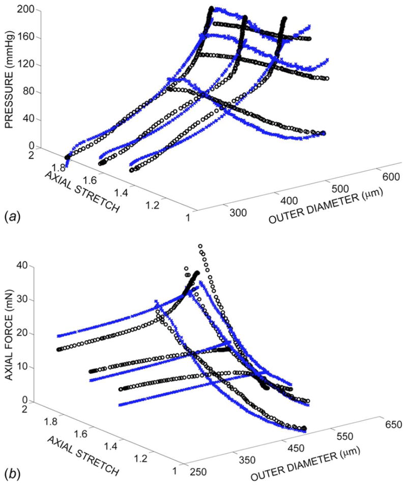
Pressure (a) and axial force (b) versus outer diameter and axial stretch. The open circles represent the experimental data and the x’s represent the model predictions using the model of Chuong and Fung [7].

Table 1.

Material parameters for the model of Chuong and Fung [7] determined via nonlinear regression

	c (kPa)	c1	c2	c3	c4	c5	c6	Error
Day 0, ${\lambda }_z^{\ast }=1.65$
053104_01	246	0.106	0.299	0.874	0.010	0.218	0.000	0.068
053104_02	140	0.077	0.433	1.158	0.011	0.278	0.000	0.067
061604_01	312	0.186	0.201	0.891	0.000	0.114	0.053	0.072
080304_02	319	0.055	0.219	0.339	0.000	0.065	0.000	0.076
100504_01	336	0.069	0.165	0.314	0.000	0.051	0.020	0.081
100504_02	333	0.073	0.175	0.285	0.000	0.036	0.027	0.099
Mean	281d	0.094d	0.249d	0.644d	0.004d	0.127d	0.017d	0.077
SD	76.4	0.048	0.102	0.376	0.005	0.099	0.021	0.012
Day 2, ${\lambda }_z^{\ast }=1.65$
053104_01	82.9	0.425	0.933	3.160	0.136	0.831	0.348	0.091
053104_02	57.9	0.287	0.915	2.718	0.092	0.728	0.229	0.092
061604_01	85.1	0.307	0.603	2.449	0.070	0.520	0.347	0.086
080304_02	62.6	0.142	0.878	1.758	0.025	0.447	0.000	0.098
100504_01	58.9	0.150	0.899	1.190	0.011	0.400	0.000	0.110
100504_02	56.3	0.379	0.744	1.518	0.062	0.286	0.188	0.093
Mean	67.3a,d	0.282d	0.829a,d	2.132d	0.066a,c,d	0.535a,d	0.185d	0.095
SD	13.1	0.116	0.129	0.762	0.045	0.206	0.157	0.008
Day 0, ${\lambda }_z^{\ast }=1.80$
060504_02	486	0.050	0.162	0.209	0.003	0.040	0.000	0.095
060804_02	991	0.047	0.093	0.088	0.000	0.002	0.001	0.078
092604_01	321	0.067	0.222	0.273	0.007	0.069	0.000	0.062
092604_02	126	0.113	0.665	2.310	0.044	0.624	0.044	0.068
100804_01	411	0.045	0.167	0.185	0.001	0.036	0.000	0.109
100804_02	295	0.049	0.204	0.195	0.000	0.039	0.005	0.083
Mean	438e	0.062e	0.252e	0.543e	0.009	0.135e	0.008	0.083
SD	297	0.026	0.207	0.868	0.017	0.241	0.018	0.017
Day 2, ${\lambda }_z^{\ast }=1.80$
060504_02	143	0.199	0.529	1.113	0.011	0.208	0.103	0.091
060804_02	185	0.175	0.458	0.742	0.020	0.148	0.057	0.080
092604_01	118	0.111	0.639	0.668	0.000	0.153	0.000	0.072
092604_02	37.4	0.216	1.275	3.706	0.019	0.908	0.080	0.074
100804_01	70.8	0.153	0.847	1.526	0.018	0.417	0.000	0.088
100804_02	54.3	0.196	0.750	0.620	0.000	0.063	0.000	0.089
Mean	101b,e	0.175e	0.750b,e	1.396e	0.011c	0.316e	0.040	0.082
SD	57.0	0.038	0.294	1.183	0.009	0.313	0.046	0.008
Day 0, ${\lambda }_z^{\ast }=1.95$
052804_01	323	0.122	0.210	0.612	0.008	0.119	0.000	0.061
052804_02	457	0.017	0.269	0.338	0.011	0.161	0.000	0.060
061204_01	270	0.128	0.281	1.043	0.031	0.244	0.085	0.074
061204_02	397	0.070	0.182	0.272	0.000	0.039	0.010	0.081
093004_01	276	0.075	0.219	0.412	0.000	0.082	0.000	0.067
Mean	345	0.082	0.232	0.535	0.010	0.129	0.019	0.069
SD	80.7	0.045	0.042	0.311	0.013	0.078	0.037	0.009
Day 2, ${\lambda }_z^{\ast }=1.95$
052804_01	381	0.164	0.190	0.677	0.000	0.072	0.121	0.135
052804_02	132	0.154	0.469	1.788	0.000	0.000	0.183	0.078
061204_01	92.9	0.291	0.675	2.056	0.000	0.303	0.311	0.147
061204_02	332	0.086	0.227	0.272	0.000	0.000	0.064	0.095
093004_01	247	0.047	0.306	0.249	0.000	0.053	0.024	0.081
Mean	237a,b	0.148	0.373a,b	1.008	0.000a	0.086a	0.141	0.107
SD	124	0.093	0.200	0.857	0.000	0.126	0.113	0.032

^aIndicates p<0.05 when comparing 1.65 and 1.95 on day 2.

^bIndicates p<0.05 when comparing 1.80 and 1.95 on day 2.

^cIndicates p<0.05 when comparing 1.65 and 1.80 on day 2.

^dIndicates p<0.05 when comparing day 0 and day 2 for the 1.65 group.

^eIndicates p<0.05 when comparing day 0 and day 2 for the 1.80 group.

Four fiber-family model

The lower and upper limits of the parameters were b and $b_1^k\in [0,{10}^5],b_2^k\in [{10}^{-4},{10}^5]$, and α ∈ [5 deg,85 deg]. Final parameter values were insensitive to initial guesses. The model provided a good fit to data with a mean value of the error=0.055 (Fig. 2). For all vessels at all culture times the fiber-family model provided a better fit than the Fung model (Table 2); this finding is consistent with that of Gleason et al. (15). A significant difference was seen for $b_1^3$ at day 2 across the low ( ${\lambda }_z^{\ast }=1.65$) and high ( ${\lambda }_z^{\ast }=1.95$) stretch culture groups and across day 0 and day 2 for low stretch culture group. Additionally, the parameter $b_2^2$ is significantly different across day 0 and day 2 for the ${\lambda }_z^{\ast }=1.80$ cultured vessels.

Fig. 2.

Pressure (a) and axial force (b) versus outer diameter and axial stretch. The open circles represent the experimental data and the x’s represent the model predictions using the four-fiber model.

Table 2.

Material parameters for the four fiber-family model determined via nonlinear regression

	b (kPa)	$b_1^1$ (kPa)	$b_2^1$	$b_1^2$ (kPa)	$b_2^2$	$b_1^3$ (kPa)	$b_2^3$	α	Error
Day 0, ${\lambda }_z^{\ast }=1.65$
053104_01	18.3	9.1	0.076	28.5	0.036	0.0068	0.986	32.5	0.037
053104_02	16.2	1.7	0.102	28.1	0.047	0.0072	0.922	31.6	0.034
061604_01	39.5	0.5	0.828	12.7	0.096	0.0000	2.463	49.4	0.038
080304_02	11.6	4.9	0.052	36.1	0.015	0.0001	1.373	31.6	0.046
100504_01	6.4	8.2	0.041	28.3	0.010	0.0000	1.627	30.7	0.054
100504_02	7.2	8.0	0.043	32.1	0.009	0.0000	1.555	37.5	0.065
Mean	16.5	5.4	0.191	27.6	0.035	0.0023b	1.488	35.5	0.046
SD	12.2	3.6	0.313	8.0	0.033	0.0036	0.559	7.2	0.012
Day 2, ${\lambda }_z^{\ast }=1.65$
053104_01	20.3	6.7	0.389	33.7	0.094	0.4074	1.063	35.0	0.064
053104_02	11.9	3.0	0.274	25.4	0.089	0.2354	0.947	32.7	0.064
061604_01	12.5	3.6	0.246	28.7	0.036	0.0119	1.228	35.3	0.044
080304_02	13.9	1.9	0.152	39.4	0.046	0.0829	0.991	26.6	0.051
100504_01	2.7	4.7	0.079	40.7	0.028	0.0941	0.973	25.5	0.071
100504_02	9.1	7.7	0.214	32.1	0.037	0.2433	0.938	32.3	0.063
Mean	11.7	4.6	0.226	33.3	0.055	0.1792a,b	1.023	31.2	0.059
SD	5.8	2.2	0.106	5.9	0.029	0.1441	0.110	4.2	0.010
Day 0, ${\lambda }_z^{\ast }=1.80$
060504_02	13.0	7.8	0.037	37.1	0.024	0.0022	0.950	41.1	0.039
060804_02	16.8	15.7	0.001	42.2	0.023	0.0010	1.263	63.8	0.043
092604_01	11.1	8.1	0.035	35.2	0.028	0.0042	0.951	40.2	0.040
092604_02	19.4	5.8	0.064	37.6	0.060	0.2072	0.687	29.9	0.048
100804_01	8.2	7.8	0.025	38.4	0.000	0.0000	2.073	13.8	0.090
100804_02	3.9	6.8	0.016	34.5	0.015	0.0001	1.148	35.1	0.055
Mean	12.1	8.7	0.030	37.5	0.025c	0.0358	1.179	37.3	0.053
SD	5.6	3.5	0.022	2.8	0.020	0.0840	0.481	16.4	0.019
Day 2, ${\lambda }_z^{\ast }=1.80$
060504_02	17.4	4.2	0.197	39.9	0.063	0.0021	1.635	36.6	0.057
060804_02	25.9	0.6	0.591	38.5	0.065	0.0389	1.227	36.3	0.046
092604_01	17.1	0.5	0.216	39.0	0.096	0.0266	1.072	33.0	0.045
092604_02	3.6	9.9	0.036	43.3	0.076	0.1153	0.968	24.3	0.049
100804_01	3.3	10.6	0.023	44.4	0.019	0.0500	1.189	24.2	0.058
100804_02	4.8	7.6	0.054	39.0	0.035	0.0530	1.045	27.0	0.055
Mean	12.0	5.6	0.186	40.7	0.059c	0.0476	1.189	30.2	0.052
SD	9.4	4.5	0.215	2.5	0.028	0.0380	0.238	5.8	0.006
Day 0, ${\lambda }_z^{\ast }=1.95$
052804_01	26.9	6.5	0.203	21.1	0.052	0.0003	1.698	41.4	0.039
052804_02	3.0	5.7	0.000	60.4	0.000	0.0828	0.605	20.5	0.037
061204_01	21.0	6.4	0.144	26.7	0.041	0.0018	1.286	35.8	0.040
061204_02	17.7	3.3	0.136	32.5	0.028	0.0000	1.727	38.6	0.047
093004_01	17.0	2.2	0.136	25.3	0.033	0.0001	1.355	36.0	0.051
Mean	17.1	4.8	0.124	33.2	0.031	0.0170	1.334	34.4	0.043
SD	8.8	1.9	0.075	15.7	0.020	0.0368	0.453	8.1	0.006
Day 2, ${\lambda }_z^{\ast }=1.95$
052804_01	23.0	3.4	0.358	21.8	0.085	0.0000	4.795	52.3	0.116
052804_02	16.4	2.6	0.117	43.2	0.097	0.0016	1.400	40.2	0.064
061204_01	12.4	2.8	0.230	41.3	0.045	0.0018	1.597	29.5	0.087
061204_02	6.4	7.8	0.021	40.0	0.055	0.0001	1.400	61.5	0.065
093004_01	2.6	4.5	0.020	42.3	0.026	0.0000	1.738	29.3	0.059
Mean	12.1	4.2	0.149	37.7	0.062	0.0007a	2.186	42.6	0.078
SD	8.0	2.1	0.145	9.0	0.029	0.0009	1.466	14.2	0.024

^ap<0.05 when comparing 1.65 and 1.95 at day 2.

^bp<0.05 when comparing day 0 and day 2 for the 1.65 group.

^cp<0.05 when comparing day 0 and day 2 for the 1.80 group.

3.2 Microstructurally Motivated Models: A Discrete Set of Fibers

We considered several variants of the rule-of-mixtures model, discussed separately below. In all cases, we prescribed the lower and upper limits of the parameters as b^e, b^m, $b_1^m,b_1^{c1}$, and $b_1^{c2}\in [0,10],b_2^m,b_2^{c1}$, and $b_2^{c2}\in [{10}^{-5},10]$, and Ω^c2|_h∈ [5 deg,85 deg]. Final parameter values were insensitive to initial guesses. For the models that included material nonuniformity, unless otherwise noted, we prescribed the limits (Rⁿ)^e/Rⁿ ∈ [0.8,0.95], (Lⁿ)^e/Lⁿ ∈ [0.8,0.95], (Rⁿ)^m/Rⁿ ∈ [0.95,1.1], (Lⁿ)^m/Lⁿ ∈ [0.95,1.1], and λ^c1|_h ∈ [1.0,1.876]. Note that these limits force elastin to be in tension in the stress-free state, collagen to be in compression in the stress-free state, and muscle may be in tension or compression. Rather than tabulating statistical differences in parameters for each variation of the rule-of-mixtures model, we instead present parameters from representative vessels from day 0 and day 2 at each culture stretch to allow comparison of the different model variations (Table 3).

Table 3.

Material parameters for representative data for various versions of the rule-of-mixtures constitutive model

	be (kPa)	bm (kPa)	$b_1^m$ (kPa)	$b_2^m$	$b_1^{cz}$ (kPa)	$b_2^{cz}$	$b_1^{c\alpha }$ (kPa)	$b_2^{c\alpha }$	ωc2	Re	$L_z^e$	Rm	$L_z^m$	λc	Error	Penalty
Day 0, ${\lambda }_z^{\ast }=1.65$ (061604_01)
ROM A (no pen)	214.9	163.4	165.0	0.034	96.2	0.107	0.0	1.895	63.2	–	–	–	–	–	0.041	–
ROM A	379.7	158.0	0.0	0.000	59.4	0.152	1.09	0.977	65.6	–	–	–	–	–	0.051	0.002
ROM B	379.8	157.2	0.0	0.008	1983	1.171	102.3	5.267	65.2	0.96	0.80	1.10	0.99	1.273	0.051	0.002
ROM C	504.9	170.1	0.0	0.000	388.6	4.331	–	–	60.0	1.00	0.80	1.10	0.95	1.222	0.081	0.006
Fiber	281.7	130.4	45.1	0.000	2345	0.751	240.0	3.436	64.7	0.92	0.80	1.10	0.95	1.303	0.056	0.002
Day 2, ${\lambda }_z^{\ast }=1.65$ (061604_01)
ROM A (no pen)	104.0	69.3	40.5	0.246	191.5	0.036	0.1	1.228	35.3	–	–	–	–	–	0.044	–
ROM A	148.5	16.7	37.3	0.060	114.8	0.136	5.4	0.570	49.4	–	–	–	–	–	0.089	0.001
ROM B	152.9	28.6	6.7	0.702	287.5	0.153	8.9	0.438	47.7	1.00	0.80	1.10	1.10	1.876	0.086	0.001
ROM C	148.7	0.0	0.0	2.341	59.7	0.361	–	–	36.4	1.00	0.80	1.10	1.09	1.760	0.129	0.006
Fiber	61.3	12.7	88.9	0.022	1700	0.548	403.0	0.985	46.8	0.90	0.80	1.10	0.95	1.433	0.101	0.008
Day 2, ${\lambda }_z^{\ast }=1.80$ (100804_02)
ROM A (no pen)	37.3	24.3	86.1	0.052	262.2	0.034	0.4	1.046	27.0	–	–	–	–	–	0.055	–
ROM A	105.3	9.2	13.3	0.158	107.4	0.205	11.5	0.446	37.8	–	–	–	–	–	0.088	0.001
ROM B	104.7	35.8	15.2	0.302	336.9	0.194	12.0	0.401	39.1	1.00	0.81	1.10	1.10	1.876	0.088	0.001
ROM C	113.4	0.0	10.5	0.401	59.4	0.329	–	–	28.1	1.00	0.80	1.10	1.09	1.809	0.135	0.004
Fiber	73.8	2.6	78.0	0.000	1878	0.967	407.0	1.248	39.8	0.95	0.80	1.10	0.95	1.406	0.113	0.010
Day 2, ${\lambda }_z^{\ast }=1.95$ (052804_02)
ROM A (no pen)	136.5	91.0	29.2	0.117	287.8	0.097	0.0	1.400	40.2	–	–	–	–	–	0.064	–
ROM A	134.2	83.1	0.0	0.000	225.0	0.153	6.8	0.348	53.3	–	–	–	–	–	0.071	0.000
ROM B	208.2	38.3	0.0	0.000	725.3	0.151	8.3	0.368	55.3	1.00	0.80	1.07	0.95	1.876	0.070	0.000
ROM C	136.9	69.6	0.3	0.888	115.9	0.261	–	–	27.8	0.95	0.80	1.10	0.95	1.783	0.122	0.009
Fiber	127.2	25.6	1.3	0.576	1730	0.352	371.7	0.244	44.1	0.95	0.80	1.10	0.95	1.584	0.087	0.000

ROM A: Uniform four-fiber: One muscle fiber, three collagen fibers (eight material parameters, one structural parameter)

Consider the rule-of-mixtures equations proposed above, but assume that the material is uniform; thus, (Rⁿ)^e=(Rⁿ)^c=(Rⁿ)^m=Rⁿ and ${(L_z^n)}^e={(L_z^n)}^c={(L_z^n)}^m=L^n$. For this case, ${\lambda }_{rr}^e={\lambda }_{rr}^c={\lambda }_{rr}^m={\lambda }_{rr},{\lambda }_{\theta \theta }^e={\lambda }_{\theta \theta }^c={\lambda }_{\theta \theta }^m={\lambda }_{\theta \theta },{\lambda }_{zz}^e={\lambda }_{zz}^c={\lambda }_{zz}^m={\lambda }_{zz}$, and

$$\begin{array}{c}{\widehat{T}}_{rr}={({\lambda }_{rr})}^2({\phi }^e{b}^e+{\phi }^m{b}^m)\\ {\widehat{T}}_{\theta \theta }={({\lambda }_{\theta \theta })}^2(({\phi }^e{b}^e+{\phi }^m{b}^m)+{\phi }^m{b}_1^m({({\lambda }_{\theta \theta })}^2-1)exp\{b_2^m{({({\lambda }_{\theta \theta })}^2-1)}^2\}+2{\phi }^c{b}_1^c{sin}^2(\alpha )[{({\lambda }^c)}^2-1]exp\{b_2^c{[{({\lambda }^c)}^2-1]}^2\})\\ {\widehat{T}}_{zz}={({\lambda }_{zz})}^2(({\phi }^e{b}^e+{\phi }^c{b}^c+{\phi }^m{b}^m)+{\phi }^e{b}_1^e({({\lambda }_{zz})}^2-1)exp\{b_2^c{({({\lambda }_{zz})}^2-1)}^2\}+2{\phi }^c{b}_1^c{cos}^2(\alpha )[{({\lambda }^c)}^2-1]exp\{b_2^c{[{({\lambda }^c)}^2-1]}^2\})\end{array}$$ (42)

Notice that this model reduces to the four fiber-family model described above; if b=(φ^eb^e+φ^mb^m), $b_1^1={\phi }^m{b}_1^m,b_2^1=b_2^m,b_1^2={\phi }^c{b}_1^{c1},b_2^2=b_2^{c1},b_1^3={\phi }^c{b}_1^{c2}$, and $b_2^3=b_2^{c2}$, then Eq. (42) is identical to Eq. (16), determined from a four fiber-family model. If we let b^e =b/(2φ^e) and b^m=b/(2φ^m), then the identical fits as above with the four fiber-family model will be achieved. The mean error for the four vessels considered was 0.055, which was equal to the mean of all vessels for the four fiber-family model; thus, these four vessels are considered representative.

We also enforced constraints (40) and (41) via the penalty method for this rule-of-mixtures model. The mean value of the error was 0.084 for the four vessels considered (Table 3), which provided a worse fit than the ROM A without penalties (i.e., the four fiber-family model), but equally well as the Fung model; these findings are consistent across all vessels (not shown). The average penalty for these four vessels was 0.001; thus, the penalty criteria were nearly, but not completely, satisfied.

ROM B. Nonuniform four-fiber: One muscle fiber, three collagen fibers (eight material parameters, seven structural parameter)

Next, consider the same functional form of the constitutive equation as in (ROM A), but let the material be nonuniform. That is, let (Rⁿ)^e/Rⁿ, (Rⁿ)^m/Rⁿ, ${(L_z^n)}^e/L^n,{(L_z^n)}^m/L^n$, λ^c1|_h = λ^c2|_h, and ω^c2|_h be free (structural) parameters that may be determined via nonlinear regression along with the eight material parameters. Note that we set ω^c1|_h =0 deg and ${\lambda }_1^c{\mid }_h={\lambda }_2^c{\mid }_h$. First, we let the upper and lower limits for the structural parameters of elastin be (Rⁿ)^e/Rⁿ ∈ [0.8,1.0] and (Lⁿ)^e/Lⁿ ∈ [0.8,1.0]; these regressions are referred to as ROM B1. The mean value of the error was 0.083 for the four vessels; the average penalty was 0.001. Thus, adding material nonuniformity provided little to no increase in the goodness of fit. Notice, too, that several of the structural parameters obtained via regression were at, or very near, the upper or lower limits prescribed for the regression. Next, we set the upper and lower limits for the structural parameters of elastin as (Rⁿ)^e/Rⁿ ∈ [0.8,0.95] and (Lⁿ)^e/Lⁿ ∈ [0.8,0.95] (denoted ROM B2); thus, elastin is required to be in tension in the mixture reference state. The mean value of the error equaled 0.100 for the four vessels, and the average penalty was 0.002. Thus, by simply requiring that elastin be in tension, there was a significant reduction in the goodness of fit. Notice, too, that whereas ${\lambda }_1^c{\mid }_h$ was at its upper limit of 1.876 for all four vessels in ROM B1, the average value for ${\lambda }_1^c{\mid }_h$ was 1.46 in ROM B2.

ROM C. Nonuniform four-fiber: One muscle fiber, three collagen fibers (six material parameters, six structural parameter)

Here we consider the same nonuniform model at ROM B, but let $b_1^{c1}=b_1^{c2}$ and $b_2^{c1}=b_2^{c2}$; that is, we let the material properties of the fibers oriented in the ω^c1|_h direction equal those oriented in the ±ω^c2|_h direction. The mean value of the error was 0.152 for the four vessels considered, and the average penalty was 0.006. Thus, requiring the collagen fibers in the axial and off-axis directions to have the same material parameters significantly reduced the goodness of fit and satisfaction of the penalty criteria.

3.3 Microstructurally Motivated Models: Distribution of Fibers

For the fiber distribution model, let R̄^e/Rⁿ, R̄^m/Rⁿ, L̄^e/Lⁿ, L̄^m/Lⁿ, λ̄^c1|_h = λ̄^c2|_h, and ω̄^c2|_h be free (structural) parameters that may be determined via nonlinear regression along with the eight material parameters and let $b_1^{c1}\ne b_1^{c2}$ and $b_2^{c1}\ne b_2^{c2}$. We used the values from ROM B2 as initial guesses for this fiber distribution. The mean value of the error equaled 0.098 for the four vessels and the average penalty was 0.005. The addition of a distribution of fibers did not appear to greatly change the goodness of fit of the model as the error values for the model were similar to ROM B2, which had the same number of free parameters. In this analysis, we fixed the width of the distribution functions by prescribing σ_p and ΔΓ for the collagen distribution and ΔR^j and ΔL^j for the elastin and muscle distribution. These parameters, however, could be adjusted to improve the goodness of fit. Ultimately, however, the utility of such microstructurally motivated model is to quantify the fiber distribution directly from data (cf. Refs. [16,17]), rather than prescribing the fiber distribution functions, as done in this paper.

4 Discussion

Mechanotransduction of mechanical signals to cellular responses plays a central role in maintaining tissue homeostasis, as well as the development of numerous pathologies. Fundamental to quantifying a mechanosensitive biological response of a cell within a tissue is the quantification of the mechanical environment in a local neighborhood around that cell. When a good approximation of the local mechanical environment (e.g., in terms of stress and strain) is made, only then can a correlation be rightfully made between local mechanical stimuli and local biological response. Thus, there is a pressing need to better quantify the local mechanical environment in blood vessels and how this local mechanical environment evolves as the tissue grows and remodels. Toward this end, we have quantified material and structural parameters for several constitutive models for mouse carotid arteries exposed to altered axial extension in organ culture.

We found that the model of Chuong and Fung [7] provided a good fit to data. However, motivated by the fact that blood vessels have smooth muscle cells oriented circumferentially and collagen fibers oriented axially and distributed at off-axis angles, we considered a microstructurally motivated four fiber-family model. In all cases the four-fiber model provided a better fit to data than did the model of Chuong and Fung [7]. Indeed, even two fiber-family models, with fibers oriented at ±α, have been shown to provide good agreement with data [3]. A four fiber-family model has been shown to provide a better fit to data from mouse vessels than a two fiber-family and a slightly better fit than a three fiber-family model [18], at the cost of additional material parameters. For the sake of improving the fit, the cost of additional parameters when using a four fiber-family over a two or three fiber-family model may not be well justified. However, when attempting to ascribe physical meaning to each fiber-family (e.g., by allowing one fiber-family to represent smooth muscle, another to represent axially oriented collagen, and others to represent collagen oriented off axis), the number of fiber-families should be chosen based on observations of the microstructure.

Although our goal in considering a four fiber-family model was to ascribe each fiber-family to a key structural constituent observed via microscopy, we found that simply performing nonlinear regression did not ensure that each fiber-family (i.e., structural constituent) contributed significantly to the mechanical response. Rather, it was necessary to employ a penalty method to ensure that each constituent had a significant contribution. Although these penalties reduced the goodness of fit compared with the nonpenalized fits, the overall goodness of fit with the penalties included was, in many cases, still equal to the fits obtained via the model of Chuong and Fung [7]; thus, fits that required each constituent be structurally significant still produced a model with reasonable agreement with data. We also found that allowing the stress-free states (or homeostatic stretches) of each constituent to be structural parameters that are solved via regression did not significantly improve model fits. Importantly, however, although this material nonuniformity did not play a significant role in improving the fit of data to our models, tracking the evolution of stress-free states of individual constituents plays a key role in quantifying microstructurally motivated models for tissue growth and remodeling [14,19,8].

Since the classic paper by Roach and Burton [11] it has been thought that elastin plays a key role in the mechanical behavior over low loads and collagen dominates the mechanical behavior over high loads. Brankov et al. [1] also suggested that elastin is under a higher strain in vivo than is collagen. Based on these observations, we imposed penalties and upper and lower limits on structural parameters that enforced these general observations. Although the imposition of these penalties and limits results in a reduction in the goodness of fit, we submit that such criteria are critical when assigning physical meaning to material and structural parameters.

Limitations of the constitutive modeling originate from the adopted assumptions. First, we modeled the mouse carotid artery as a homogeneous mixture. It is clear, however, that these vessels have a thin intima consisting of an endothelial cell monolayer on a basement membrane, a media consisting of smooth muscle, elastin, and collagen, and an adventitia dominated by fibroblasts and collagen; thus vessels are heterogeneous. Unfortunately, sufficient data are not available on the distribution of the key structural constituents and how the content and organization of these constituents evolve during remodeling to altered axial stretch in this ex vivo setting. Although these data are not currently available, as data become available, the structurally motivated models are capable of accounting for vessel heterogeneity by incorporating experimentally observable spatial and temporal variations in structural parameters. Second, because the opening angle was not measured in Ref. [5], we assumed that the strain was uniform across the wall in the in vivo configuration; this assumption may be tested as data on the evolution of opening angle during stretch-induced remodeling become available. Third, and more fundamental, is the assumption that the overall stress is given as the sum of the stresses borne by the individual constituents in the fiber-family and rule-of-mixtures models, thus, excluding the contribution of constituent-to-constituent interactions. Ultimately, incorporation of such interactions will provide important insights toward mechanobiology; however, sufficient data are not yet available to motivate reasonable functional forms for such constitutive equations. Finally, we model the tissue as a constrained mixture; thus, each constituent is constrained to follow the motion of the tissue on the whole; this need not be (and likely is not) the case. To overcome all of these limitations, there is a need for data that quantifies the spatial and temporal variations of constituent content and organization with remodeling and mechanical loading.

In conclusion, we have identified material (and structural) parameters for phenomenological and microstructural models of mouse common carotid arteries exposed to altered axial extension, ex vivo. We have identified models with parameters that provide good agreement with data, while ascribing physical and microstructural meaning to fiber-families that are associated with the underlying microstructural content and organization of the tissue. Although we made several assumptions (e.g., homogeneity, uniform strain in vivo, etc.), as data become available these assumptions may be relaxed. Through the application of new imaging strategies, experimental quantification of spatial and temporal variations in microstructural parameters promises to yield models with broader capabilities to predict the evolution of mechanical behavior during growth and remodeling associated with physiological and pathophysiological processes.

References

- 1.Brankov G, Rachev AI, Stoychev S. A Composite Model of Large Blood Vessels. In: Brankov G, editor. Mechanics of Biological Solid: Proceedings of the Euromech Colloquium. Bulgarian Academy of Sciences; Varna, Bulgaria: 1975. pp. 71–78. [Google Scholar]
- 2.Lanir Y. Constitutive Equations for Fibrous Connective Tissues. J Biomech. 1983;16:1–12. doi: 10.1016/0021-9290(83)90041-6. [DOI] [PubMed]
- 3.Holzapfel GA, Gasser TC, Ogden RW. A New Constitutive Framework for Arterial Wall Mechanics and a Comparative Study of Material Models. J Elast. 2000;61:1–48. [Google Scholar]
- 4.Zulliger MA, Fridez P, Hayashi K, Stergiopulos N. A Strain Energy Function for Arteries Accounting for Wall Composition and Structure. J Biomech. 2004;37:989–1000. doi: 10.1016/j.jbiomech.2003.11.026. [DOI] [PubMed] [Google Scholar]
- 5.Gleason RL, Wilson E, Humphrey JD. Biaxial Biomechanical Adaptations of Mouse Carotid Arteries Cultured at Altered Axial Extension. J Biomech. 2007;40:766–776. doi: 10.1016/j.jbiomech.2006.03.018. [DOI] [PubMed] [Google Scholar]
- 6.Baek S, Gleason RL, Rajagopal KR, Humphrey JD. Theory of Small on Large in Computations of Fluid-Solid Interactions in Arteries. Comput Methods Appl Mech Eng. 2007;196:3070–3078. [Google Scholar]
- 7.Chuong CJ, Fung YC. On Residual Stress in Arteries. ASME J Biomech Eng. 1986;108:189–192. doi: 10.1115/1.3138600. [DOI] [PubMed] [Google Scholar]
- 8.Gleason RL, Taber LA, Humphrey JD. A 2-D Model of Flow-Induced Alterations in the Geometry, Structure, and Properties of Carotid Arteries. ASME J Biomech Eng. 2004;126:371–381. doi: 10.1115/1.1762899. [DOI] [PubMed] [Google Scholar]
- 9.Humphrey JD. Cardiovascular Solid Mechanics: Cells, Tissues, Organs. Springer-Verlag; New York: 2002. [Google Scholar]
- 10.Spencer AJM. Constitutive Theory for Strongly Anisotropic Solids. In: Spencer AJM, editor. Continuum Theory of the Mechanics of Fibre-Reinforced Composites (CISM Courses and Lectures Vol. 282) Springer-Verlag; Wien: 1984. pp. 1–32. [Google Scholar]
- 11.Roach M, Burton A. The Reason for the Shape of the Distensibility Curves of Arteries. Can J Biochem Physiol. 1957;35:681–690. [PubMed] [Google Scholar]
- 12.Azeloglu EU, Albro MB, Thimmappa VA, Ateshian GA, Costa KD. Heterogeneous Transmural Proteoglycan Distribution Provides a Mechanism for Regulating Residual Stresses in the Aorta. Am J Physiol Heart Circ Physiol. 2008;294(3):H1197–H1205. doi: 10.1152/ajpheart.01027.2007. [DOI] [PubMed] [Google Scholar]
- 13.Martinez-Lemus LA, Hill MA, Bolz SS, Pohl U, Meininger GA. Acute Mechanoadaptation of Vascular Smooth Muscle Cells in Response to Continuous Arteriolar Vasoconstriction: Implications for Functional Remodeling. FASEB J. 2004;18(6):708–710. doi: 10.1096/fj.03-0634fje. [DOI] [PubMed] [Google Scholar]
- 14.Gleason RL, Humphrey JD. A 2-D Constrained Mixture Model for Arterial Adaptations to Large Changes in Flow, Pressure, and Axial Stretch. Math Med Biol. 2005;22(4):347–369. doi: 10.1093/imammb/dqi014. [DOI] [PubMed] [Google Scholar]
- 15.Gleason RL, Dye WW, Wilson E, Humphrey JD. Quantification of the Mechanical Behavior of Carotid Arteries From Wild-Type, Dystrophin-Deficient, and Sarcoglycan-Delta Knockout Mice. J Biomech. 2008;41(15):3213–3218. doi: 10.1016/j.jbiomech.2008.08.012. [DOI] [PMC free article] [PubMed] [Google Scholar]
- 16.Gleason RL, Wan W. Theory and Experiments for Mechanically-Induced Remodeling of Tissue Engineered Blood Vessels. Adv Sci Technol. 2008;57:226–234. [Google Scholar]
- 17.Wicker B, Hutchens H, Wu Q, Yeh A, Humphrey J. Normal Basilar Artery Structure and Biaxial Mechanical Behavior. Comput Methods Biomech Biomed Eng. 2008;11(5):539–551. doi: 10.1080/10255840801949793. [DOI] [PubMed] [Google Scholar]
- 18.Zeinali-Davarani S, Choi J, Baek S. On Parameter Estimation for Biaxial Mechanical Behavior of Arteries. J Biomech. 2009;42(4):524–530. doi: 10.1016/j.jbiomech.2008.11.022. [DOI] [PubMed] [Google Scholar]
- 19.Humphrey JD, Rajagopal KR. A Constrained Mixture Model for Growth and Remodeling of Soft Tissues. Math Models Meth Appl Sci. 2002;12(3):407–430. [Google Scholar]