Modeling Relations Among Discrete Developmental Processes: A General Approach to Associative Latent Transition Analysis

Abstract

To understand one developmental process, it is often helpful to investigate its relations with other developmental processes. Statistical methods that model development in multiple processes simultaneously over time include latent growth curve models with time-varying covariates, multivariate latent growth curve models, and dual trajectory models. These models are designed for growth represented by continuous, unidimensional trajectories. The purpose of this article is to present a flexible approach to modeling relations in development among two or more discrete, multidimensional latent variables based on the general framework of loglinear modeling with latent variables called associative latent transition analysis (ALTA). Focus is given to the substantive interpretation of different associative latent transition models, and exactly what hypotheses are expressed in each model. An empirical demonstration of ALTA is presented to examine the association between the development of alcohol use and sexual risk behavior during adolescence.

It is often helpful to investigate relations between two developmental processes. For example, improved understanding of whether and how development in alcohol use is linked to development in sexual behavior could inform programs to prevent sexually transmitted infections (STIs), including HIV/AIDS. There have been notable advances in statistical methods for modeling development in multiple processes simultaneously over time. These include latent growth curve models with time-varying covariates (Bollen & Curran, 2006), dual latent growth curve models (Willett & Sayer, 1996), multivariate latent growth curve models (Bollen & Curran, 2006), and dual trajectory analysis (Nagin, 2005). All of these modeling approaches are appropriate for studying the link between processes that can be represented by continuous, unidimensional trajectories. The current article describes a general modeling approach appropriate for studying the link between two discrete processes.

Recently, approaches to modeling development in a discrete process based on latent class analysis (LCA) have become popular. LCA is a statistical method that has been widely used to identify subgroups of individuals (i.e., classes) characterized by similar multidimensional patters of responses (Goodman, 1974; Clogg, 1995; Lazarsfeld & Henry, 1968; Collins & Lanza, in press). In LCA, a mathematical model relates discrete manifest variables to a single discrete latent variable. A longitudinal extension of LCA, latent transition analysis (LTA) models change in a single discrete latent variable over two or more times (Collins & Wugalter, 1992; Collins & Lanza, in press; Lanza, Flaherty, & Collins, 2003; Lanza, Collins, Schafer, & Flaherty, 2005; Lanza & Collins, 2008).

Many applications of LCA and LTA to alcohol and drug use can be found in the literature in the social and behavioral sciences (e.g., Reboussin, Song, Shrestha, Lohman, & Wolfson, 2006; Biemer & Wiesen, 2002, Guo, Collins, Hill, & Hawkins, 2000; Collins, Graham, Rousculp, & Hansen, 1997; Chung, Park, & Lanza, 2005; Whitesell, Beals, Mitchell, Novins, Spicer, et al., 2006; Monga, Rehm, Fischer, Brissette, Bruneau, et al., 2007), and these applications illustrate how latent class methods may be used to develop a rich, multidimensional picture of development. These methods have been used to identify subgroups of individuals with similar patterns of alcohol use, as well as to model change over time in alcohol use. For example, Lanza et al. (2007) used seven indicators of drinking behavior (e.g., past-year alcohol use, past-month alcohol use, five or more drinks in a row during the last two weeks) to identify five latent classes of alcohol use among high school seniors. These latent classes were labeled non-drinkers, experimenters, drinkers, occasional bingers and heavy drinkers. In another application, Auerbach and Collins (2006) used four indicators of drinking behavior (e.g., past-year alcohol use, past-month frequency of alcohol use, heavy episodic drinking) to identify five latent classes of alcohol use, and to explore change over time in alcohol use during emerging adulthood.

A few studies have taken a discrete, multidimensional approach to identifying subgroups of individuals with similar patterns of sexual behavior, as well as to modeling change over time in sexual behavior. For example, Newman and Zimmerman (2000) used cluster analysis to identify four subgroups of individuals based on condom use and number of partners. In another example, Beadnell, Morrison, Wilsdon, Wells, Murowchick, et al. (2005) used latent profile analysis to identify latent classes of sexual behavior based on condom use, number of partners, and frequency of sex. Lanza and Collins (2008) used four indicators of dating and sexual behavior (e.g., number of dating partners, past-year sexual behavior, condom use) and LTA to identify five latent classes of sexual behavior, and to model change over time in sexual behavior. In addition, Lanza and Collins briefly discussed some of the advantages to taking a multidimensional approach to studying sexual behavior. For example, subgroups of individuals who are at varying levels of risk for contracting an STI can be identified based on a set of behavioral indicators.

The use of LCA and LTA in these areas has provided valuable information about the development of alcohol use and sexual behavior separately. Additional insight can be gained by examining whether and how change in the two processes may be related. Recently, Flaherty (2008a,b) proposed a variation of LTA called associative latent transition analysis (ALTA) that can be used to model associations between transitions in latent class membership for two processes. Flaherty (2008a) used ALTA to test hypotheses about the association between tobacco use development and alcohol use development, and Flaherty (2008b) examined the association between psychological state and substance use over time. In the latter application, four models specifying different degrees of dependence between psychological state and substance use were considered: independence, cross-sectional association, longitudinal association, and full association. This approach also has been used to model the association between negative affect and alcohol use (Witkiewitz & Villarroel, 2009).

Purpose of the Current Article

The purpose of this article is to extend Flaherty's work by presenting a flexible approach to modeling the structural relations among two or more discrete developmental processes simultaneously over time, based on the general framework of loglinear modeling with latent variables (e.g., Hagenaars, 1993). This enables fitting a broader array of models, opening up new possibilities for testing hypotheses about growth and change. The empirical demonstration used here examines the association between development in alcohol use and development in sexual behavior among high school seniors. Both alcohol use and sexual behavior are modeled as longitudinal latent class variables.

Loglinear modeling with manifest and latent variables, including LCA and LTA, will be introduced. Then, the first of two studies will be described. In Study I, LTA will be used to model development in alcohol use and sexual behavior separately. Loglinear modeling with latent variables will be used as a general framework for ALTA. The seven ALTA models considered illustrate a subset of the possible models that can be fit using this framework. As will be demonstrated, some of the models differ in subtle ways that are not readily apparent from probabilities describing transitions in sexual behavior conditional on transitions in alcohol use; they can be distinguished only by examining the relative odds of particular transitions in behavior. Then, the second study will be described. In Study II, the alcohol use and sexual behavior models from Study I will be linked in the seven different ways hypothesized by the ALTA models.

Loglinear Modeling with Manifest and Latent Variables

Loglinear models are generalized linear models for contingency tables. Contingency tables cross-tabulate data from multiple discrete variables. In loglinear models, observed contingency table data depend on associations and interactions among levels of discrete variables. A brief discussion of loglinear modeling with manifest variables is presented below to introduce the notation that will be used throughout the current article. More complete discussions of loglinear modeling may be found in many classic texts on categorical data analysis, including Agresti (2002) and Bishop, Fienberg, and Holland (1975).

Consider two discrete variables A and B that have i = 1, … , I and j = 1, … , J response categories, respectively. The resulting two-way, I × J contingency table contains IJ cells with expected cell counts denoted by μ_ij and the total sample size denoted by N. In a two-way table, the most general model, called the saturated model, has the loglinear expression

$$\log {\mu }_{ij}={\lambda }_0+{\lambda }_i^A+{\lambda }_j^B+{\lambda }_{ij}^{AB},$$ (1)

where λ₀ is an intercept and a normalizing constant to ensure ${\Sigma }_{i=1}^I{\Sigma }_{j=1}^J{\mu }_{ij}=N$, ${\lambda }_i^A$ is the effect of level i of variable A, ${\lambda }_j^B$ is the effect of level j of variable B, ${\lambda }_{ij}^{AB}$ is the interactive effect of level i of variable A and level j of variable B that reflects a deviation from independence, and model identifiability requires constraints such as ${\lambda }_I^A={\lambda }_J^B=0$ (Agresti, 2002, pg. 315). In general, the saturated model fits the data perfectly, as it includes all possible interactions. The saturated model is hierarchical in that it includes all lower-order terms (${\lambda }_i^A$ and ${\lambda }_j^B$) involved in the higher-order interaction term (${\lambda }_{ij}^{AB}$; Agresti, 2002).

The loglinear model discussed may be directly extended to multi-way tables, but the set of all possible hierarchical¹ models increases exponentially. When addressing research questions about the relations among three or more discrete variables, a small subset of models that correspond to theoretically logical, hypothesized relations among the variables may be selected. In practice, often only hierarchical models are considered, but non-hierarchical models may be useful for some research questions (Rindskopf, 1990). Only hierarchical models are considered in the current article. Because they are nested, hierarchical loglinear models may be compared using likelihood ratio tests. They also may be compared using criteria like the Akaike Information Criterion (AIC; Akaike, 1974) and Bayesian Information Criterion (BIC; Schwartz, 1978).

A convenient shorthand notation is commonly used in which a hierarchical loglinear model is referred to by a symbol that lists the highest-order terms for each variable (Agresti, 2002). Using the shorthand notation, the saturated model may be written (AB), which implies that the main effects of A and B, as well as the interactive effect of A and B (AB), are included in the model for μ_ij. A model in which A and B are assumed to be independent may be written (A, B), which implies that only the main effects of A and B are included in the model. This shorthand notation is used throughout the current article.

Latent Class and Latent Transition Analysis

Loglinear models may be used to characterize associations and interactions among discrete latent variables measured by discrete manifest items. LCA, LTA and ALTA are all types of loglinear modeling with latent variables that use manifest items with discrete response options to divide a population into a set of mutually exclusive and exhaustive discrete latent classes based on the observed contingency table data (Goodman, 1974; Clogg, 1995; Collins & Lanza, in press; Lanza et al., 2003; Lazarsfeld & Henry, 1968). Loglinear modeling with latent variables can be used to examine: (a) the ways in which discrete manifest items are probabilistically related to discrete latent variables, and (b) the ways in which discrete latent variables are associated. The former is often referred to as the measurement model; the latter, which is often referred to as the structural model, is of primary interest in this article. In LCA, loglinear modeling is used to examine the measurement models of latent class variables. In LTA and ALTA, loglinear modeling is used to examine the associations among two or more latent class variables, as well as their measurement models. More complete discussions of loglinear modeling with latent variables may be found in, for example, Hagenaars (1988, 1992, 1993, 1994), Heinen (1996), Everitt and Dunn (1988), and Vermunt (1996).

In LCA, the latent class mathematical model may be expressed in loglinear terms. For example, suppose there are four discrete variables A, B, C and D measuring sexual behavior as a discrete latent variable S. Then, the latent class mathematical model in loglinear notation is (AS,BS,CS,DS). This notation indicates that the four variables are directly related to the latent variable but not to each other. The assumption that the manifest variables are related to each other only through their relation to the latent variable is known as local independence. Additional details of the latent class model may be found in a variety of resources including Goodman (1974), Clogg (1995), Collins and Lanza (in press), Lanza et al. (2007), and Chung, Flaherty, and Schafer (2006).

LTA is used to model change over time in a discrete latent variable (Collins & Wugalter, 1992; Collins & Lanza, in press; Lanza et al., 2003; Lanza & Collins, 2008). In LTA, latent class membership is dynamic; that is, participants may transition between latent classes over time. If sexual behavior is measured at two times, the (structural) model in loglinear notation is (S₁S₂), where the subscripts denote time, implying S₁ and S₂ are related. There is a latent class measurement model in place within each time, but the focus from this point forward is only on the structural model. The interaction between S₁ and S₂ expressed by (S₁S₂) is reflected in the set of joint probabilities P (S₁ = x, S₂ = y), where x and y are sexual behavior latent classes at time 1 (S₁ = 1, … ,X) and time 2 (S₂ =1, … ,Y), respectively. Additional details and empirical demonstrations of the latent transition model may be found in a variety of resources including Collins and Lanza (in press), Lanza and Collins (2008), Lanza et al. (2005), and Chung et al. (2005). For ease of exposition in the remainder of this article, alcohol use measured at two times is labeled A₁ and A₂. An underlying latent class measurement model is assumed for each discrete latent variable.

An alternative parameterization of LCA and LTA based on probabilities may be more familiar to some readers. This parameterization of LCA is defined by two sets of probabilities. Latent class membership probabilities are unconditional probabilities of membership in the latent classes; they comprise the structural model. Item-response probabilities are the probabilities of particular responses to particular items conditional on latent class membership; they comprise the measurement model. LTA is additionally defined by a third set of parameters. Transition probabilities are the probabilities of latent class membership at time t + 1 conditional on latent class membership at time t. In LTA, the latent class membership and transition probabilities together comprise the structural model and the item-response probabilities comprise the measurement model. The association between S₁ and S₂ is reflected in the transition probabilities, which are conditional probabilities calculated from the joint probabilities,

$$P(S_2=y\mid S_1=x)=\frac{P(S_1=x,S_2=y)}{{\Sigma }_{k=1}^X{S}_1=k}.$$ (2)

A brief comparison of the loglinear and probability parameterizations of the latent class model is found in Hagenaars (1993).

Study I: Modeling Transitions in Alcohol Use and Sexual Behavior

Participants

Data for the current study were from Rounds 2 and 3 of the National Longitudinal Survey of Youth, 1997 (NLSY97; Bureau of Labor Statistics, 2007). The NLSY97 is sponsored and directed by the U.S. Bureau of Labor Statistics and conducted by the National Opinion Research Center at the University of Chicago, with assistance from the Center for Human Resource Research at The Ohio State University. The sample used in the current study consisted of 2,255 adolescents assessed at age 17 or 18 in 1998, and then assessed again in 1999. The sample was the same as that of Lanza and Collins (2008), but included only participants who provided complete data on all measures of alcohol use and sexual behavior at both time points. A total of 682 incomplete cases were excluded to simplify the later ALTA analyses. The sample comprised 50% males and 50% females, with 58% White, 27% African American, 2% Asian or Pacific Islander, and 13% other race/ethnicities.

Measures

Three questionnaire items were used to measure alcohol use: alcohol use in the past year (no, yes); alcohol use in the past month (no, yes); and binge drinking in the past month (no, yes), defined as drinking five or more drinks per day on one or more days in the last 30 days.

Four questionnaire items were used to measure sexual behavior: number of dating partners in the past year (0, 1, 2 or more); sexual intercourse in the past year (no, yes); number of sexual partners in the past year (0, 1, 2 or more); and report of at least one instance of intercourse without use of a condom (i.e., possible exposure to STI s) in the past year (no, yes).

Analysis

First, a latent transition model of alcohol use was selected. This model identified types of alcohol users and described change over time in alcohol use. The approach used to develop and select the latent transition model was similar to the one discussed in detail by Lanza and Collins (2008). Model selection was based on the G² fit statistic, AIC, BIC, and substantive interpretations of the models; measurement invariance across time was imposed on all models. To ensure identification of the maximum likelihood solution, 100 sets of random starting values were used. Second, the sexual behavior model described in Lanza and Collins (2008) was replicated using LCA and LTA, to ensure that essentially the same model held in the reduced sample.

Results

Alcohol Use

A three-class model was selected to describe transitions over time in alcohol use. A complete summary of the LTA parameter estimates, including the item-response probabilities, latent class membership probabilities and transition probabilities, is shown in Table 1. The results presented with participants who provided complete data were similar to those based on all participants (not shown).

Table 1.

Alcohol Use Latent Transition Analysis (LTA) Results

		Non-drinkers	Experimenters	Binge Drinkers
Latent Class	Time 1	0.419	0.308	0.273
Membership Probabilities	Time 2	0.365	0.271	0.364
	Item-response Probabilities
Past-year alcohol use	No	0.937	0.000	0.000
	Yes	0.063	1.000	1.000
Past-month alcohol use	No	1.000	0.465	0.000
	Yes	0.000	0.535	1.000
Past-month binge drinking	No	1.000	1.000	0.129
	Yes	0.000	0.000	0.871

Transition Probabilities	Time 2 Latent Class Membership
Time 1 Latent Class Membership	Non-drinkers	Experimenters	Binge Drinkers
Non-drinkers	0.703	0.181	0.117
Experimenters	0.157	0.520	0.323
Binge Drinkers	0.080	0.129	0.791

The item-response probabilities suggested the following labels for the three latent classes of alcohol use: Non-drinkers, Experimental Drinkers, and Binge Drinkers. Non-drinkers were characterized by high probabilities of reporting no drinking in the past year (0.937), no drinking in the past month (1.000), and no binge drinking in the past month (1.000). Experimental Drinkers were characterized by a high probability of reporting drinking in the past year, a moderate probability of drinking in the past month (0.535), and a low probability of binge drinking in the past month. Binge Drinkers were characterized by high probabilities of reporting drinking in the past year, drinking in the past month, and binge drinking in the past month (0.871).

The transition probabilities shown in Table 1 suggest that probabilities of membership in the Non-drinkers and Experimental Drinkers latent classes decreased slightly over time whereas the probability of membership in the Binge Drinkers latent class increased over time (0.273 to 0.364). Non-drinkers and Binge Drinkers had high stability over time, meaning that they were likely to be in the same latent class over time (0.703 and 0.791). Experimental Drinkers were less stable in their behavior, and Experimental Drinkers who transitioned to another latent class were most likely to transition to the Binge Drinking latent class (0.323).

Sexual Behavior

The five-class model of dating and sexual risk behavior presented in Lanza and Collins (2008) was replicated with participants who provided complete data on the variables used in the current study. A complete summary of the LTA parameter estimates, including the item-response probabilities, latent class membership probabilities and transition probabilities, is shown in Table 2. These results are similar to those based on all participants (Lanza & Collins, 2008).

Table 2.

Sexual Behavior Latent Transition Analysis (LTA) Results

		Non-daters	Daters	Monog	M-P Safe	M-P Exp
Latent Class	Time 1	0.153	0.307	0.132	0.117	0.238
Membership Probabilities	Time 2	0.206	0.257	0.219	0.113	0.258
	Item-response Probabilities
Past-year number of dating partners	0	0.763	0.001	0.071	0.042	0.026
	1	0.154	0.195	0.576	0.035	0.042
	2 or more	0.083	0.804	0.352	0.923	0.932
Past-year sex	No	1.000	1.000	0.000	0.000	0.000
	Yes	0.000	0.000	1.000	1.000	1.000
Past-year number of sexual partners	0	1.000	1.000	0.000	0.000	0.000
	1	0.000	0.000	0.994	0.380	0.089
	2 or more	0.000	0.000	0.006	0.620	0.911
Past-year exposure to STI	No	1.000	1.000	0.453	1.000	0.284
	Yes	0.000	0.000	0.547	0.000	0.717

Transition Probabilities	Time 2 Latent Class Membership
Time 1 Latent Class Membership I	Non-daters	Daters	Monog	M-P Safe	M-P Exp
Non-daters	0.659	0.174	0.076	0.040	0.052
Daters	0.001	0.622	0.186	0.100	0.091
Monogamous	0.048	0.040	0.663	0.036	0.213
Multipartner Safe	0.049	0.127	0.176	0.586	0.062
Multipartner Exposed	0.023	0.043	0.162	0.000	0.773

Note: Monog is monogamous; M-P Safe is multipartner safe; M-P Exp is multipartner exposed.

The five latent classes were labeled: Non-daters, Daters, Monogamous, Multipartner Safe, and Multipartner Exposed. Non-daters were characterized by high probabilities of reporting 0 dating partners in the past year (0.763), no sex in the past year (1.000), 0 sexual partners in the past year (1.000), and no STI exposure in the past year (1.000). Daters were characterized by high probabilities of reporting 2 or more dating partners in the past year (0.804), no sex in the past year, 0 sexual partners in the past year, and no STI exposure in the past year. Monogamous individuals were characterized by high probabilities of reporting having had 1 sexual partner in the past year (0.994), and they may or may not have been exposed to STIs in the past year (0.547 were exposed). Multipartner Safe and Multipartner Exposed individuals had high probabilities of reporting having had 2 or more sexual partners in the past year, but Safe individuals had a high probability of no exposure to STIs in the past year (1.000) whereas Exposed individuals had a high probability of exposure to STIs in the past year (0.717).

The transition probabilities shown in Table 2 suggest that probability of membership in the Daters latent class decreased slightly over time (0.307 to 0.257), whereas the probability of membership in the Monogamous latent class increased slightly over time (0.132 to 0.219). The probabilities of membership in the Multipartner Safe and Multipartner Exposed latent classes stayed approximately the same. Daters who transitioned to another latent class were most likely to transition to the Monogamous latent class (0.186), and were approximately equally (but less) likely to transition to the Multipartner Safe and Multipartner Exposed latent classes (0.100 and 0.091). Monogamous individuals who transitioned to another latent class were most likely to transition to the Multipartner Exposed latent class (0.213), and they were at highest risk overall for transitioning to this high-risk latent class.

Any conclusions about change over time in alcohol use or sexual behavior are based on the transition probabilities. For example, the transition probability P (S₂ = Multipartner Exposed|S₁ = Monogamous) = 0.213 implies that 21.3% of Monogamous individuals at time 1 transitioned to Multipartner Exposed at time 2. Typically, the transition probabilities are used to describe how individuals change over time. Alternatively, change over time may be described using conditional odds and odds ratios. For example, the conditional odds

$$\frac{P(S_2=\text{Multipartner Exposed}\mid S_1=\text{Monogamous})}{P(S_2=\text{Multipartner Safe}\mid S_1=\text{Monogamous})}=\frac{0.213}{0.036}=5.917$$ (3)

expresses that the odds of transitioning to Multipartner Exposed in reference to Multipartner Safe at time 2 for Monogamous individuals at time 1 was approximately 6:1. In addition, conditional odds ratios can be used to compare the odds of transitioning between latent classes (as expressed in Equation 3) for individuals in different latent classes at time 1. For example, the odds ratio for transitioning to Multipartner Exposed in reference to Multipartner Safe for Monogamous individuals compared to Daters was

$$\frac{\frac{P(S_2=\text{Multipartner Exposed}\mid S_1=\text{Monogamous})}{P(S_2=\text{Multipartner Safe}\mid S_1=\text{Monogamous})}}{\frac{P(S_2=\text{Multipartner Exposed}\mid S_1=\text{Daters})}{P(S_2=\text{Multipartner Safe}\mid S_1=\text{Daters})}}=6.502.$$ (4)

This means that the odds of transitioning to Multipartner Exposed in reference to Multipartner Safe at time 2 were 6.5 times higher for Monogamous individuals compared to Daters at time 1. Although conditional odds and odds ratios are not often used for interpretation in LTA, they play an important role in ALTA, which is discussed in Study II.

ALTA

In Study I, separate LTA models of transitions in alcohol use and sexual behavior were presented. In Study II, the use of ALTA to model the relation between development in alcohol use and development in sexual behavior will be demonstrated. In ALTA, many parameters are estimated although only a subset are typically of interest. To narrow the scope of Study II, the discussion below focuses on a subset of parameters. The following questions are addressed: (a) How do sexual behavior transition probabilities differ by baseline alcohol use and by transitions in alcohol use over time? and (b) What is the change in odds of transitioning to Multipartner Exposed in reference to Multipartner Safe for Monogamous individuals compared to Daters, for individuals who change their alcohol use over time? In other words, how do transitions in alcohol use differentially predict transitions to Exposed versus Safe multipartner sexual behavior for individuals who were Monogamous at the start of the study, and those who were Daters. Addressing these questions may help prevention and public health researchers understand how different transitions in alcohol use may be differentially associated with the transition from low-risk sexual behavior (e.g., Monogamous) to high-risk sexual behavior (e.g., Multipartner Exposed).

Seven models of association between alcohol use and sexual behavior are considered mathematically and discussed in terms of substantive conclusions. The models considered here illustrate the variety of models that can be fit using the ALTA approach, and how a set of ALTA models can be used to address specific research questions related to development.

There are a variety of ways in which development in one process may be related to development in others. For example, it may be that the two processes are associated at each time, but that transitions in one process are not associated with transitions in the other. Alternatively, it may be that transitions in one process are associated with higher probabilities of making particular transitions (compared to others) in the other processes. Different hypothesized associations between alcohol use and sexual behavior correspond to different ALTA models that can be expressed by placing corresponding patterns of restrictions on probabilities and/or odds ratios. Here, seven ALTA models are considered. All models are discussed as if data are from two measurement occasions, but the models may be directly extended to three or more times.

To address the questions posed above, the discussion of the seven models focuses on the way in which alcohol use at time 1 and transitions in alcohol from time 1 to time 2 were associated with transitions from low-risk to high-risk sexual behavior. For example, consider comparing individuals who transitioned from Non-drinking to Binge Drinking to individuals who remained in the Non-drinkers latent class over time. In Study I, both transition probabilities and odds ratios were used to describe change over time in sexual behavior. The probability of transitioning from the Monogamous latent class to the Multipartner Exposed latent class, P (S₂ = Multipartner Exposed|S₁ = Monogamous), was examined because it represents a transition from low-risk to high-risk sexual behavior. Here, the probability of transitioning from the Monogamous to Multipartner Exposed latent class among individuals who transitioned from Non-drinking to Binge Drinking,

$$P(S_2=\text{Multipartner Exposed}\mid S_1=\text{Monogamous},A_1=\text{Non-drinker},A_2=\text{Binge Drinker}),$$ (5)

was compared to the corresponding one among individuals who remained in the Non-drinkers latent class over time,

$$P(S_2=\text{Multipartner Exposed}\mid S_1=\text{Monogamous},A_1=\text{Non-drinker},A_2=\text{Non-drinker}).$$ (6)

Similarly, in Study I, the odds ratio expressing the change in odds of transitioning to Multipartner Exposed in reference to Multipartner Safe for Monogamous individuals compared to Daters was also examined. Here, the odds ratio of transitioning to Multipartner Exposed in reference to Multipartner Safe for Monogamous individuals compared to Daters among individuals who transitioned from Non-drinking to Binge Drinking,

$$\frac{\frac{P(S_2=\text{Multipartner Exposed}\mid S_1=\text{Monogamous},A_1=\text{Non-drinking},A_2=\text{Binge Drinking})}{P(S_2=\text{Multipartner Safe}\mid S_1=\text{Monogamous},A_1=\text{Non-drinking},A_2=\text{Binge Drinking})}}{\frac{P(S_2=\text{Multipartner Exposed}\mid S_1=\text{Daters},A_1=\text{Non-drinking},A_2=\text{Binge Drinking})}{P(S_2=\text{Multipartner Safe}\mid S_1=\text{Daters},A_1=\text{Non-drinking},A_2=\text{Binge Drinking})}},$$ (7)

was compared to the corresponding one among individuals who who remained in the Non-drinkers latent class over time,

$$\frac{\frac{P(S_2=\text{Multipartner Exposed}\mid S_1=\text{Monogamous},A_1=\text{Non-drinking},A_2=\text{Non-drinking})}{P(S_2=\text{Multipartner Safe}\mid S_1=\text{Monogamous},A_1=\text{Non-drinking},A_2=\text{Non-drinking})}}{\frac{P(S_2=\text{Multipartner Exposed}\mid S_1=\text{Daters},A_1=\text{Non-drinking},A_2=\text{Non-drinking})}{P(S_2=\text{Multipartner Safe}\mid S_1=\text{Daters},A_1=\text{Non-drinking},A_2=\text{Non-drinking})}}.$$ (8)

The nature of and extent to which alcohol use and sexual behavior are hypothesized to relate vary the extent to which probabilities and odds ratios describing transitions in sexual behavior differ for individuals with different types of alcohol use at time 1, or with different transitions in alcohol use from time 1 to time 2. A relatively weak association may be able to be characterized by an ALTA model that is more heavily restricted, allowing for fewer differences in sexual behavior for individuals with different types of alcohol use and different transitions in alcohol use. In contrast, a relatively strong association between alcohol use and sexual behavior may require a model that is less heavily restricted, estimating more parameters that reflect differences in sexual behavior among individuals with different types of alcohol use and different transitions in alcohol use.

The ALTA models selected for consideration in the current study allow for choosing a model that logically and optimally reflects the association between change over time in alcohol use and sexual behavior. The seven ALTA models presented here have been divided into two sets and are presented in order of increasing complexity in terms of modeling the association between alcohol use and sexual behavior. As the models become more complex, different effects are added to allow for additional associations and interactions between the two processes over time. This approach to model specification starts with a model that is highly restricted and removes restrictions to increase model complexity.²

The first set comprises three models, Models 1–3, that are expressed by placing restrictions directly on probabilities. The second set comprises three models, Models 4–6, that are expressed by placing restrictions on odds ratios rather than probabilities. Model 7 is (structurally) unrestricted. A summary of the patterns of restrictions placed on the probabilities for Models 1–3 is shown in Table 3. A summary of the restrictions placed on the odds ratios for Models 4–6 is shown in Table 4. Model 7 is unrestricted and is included in both tables for comparison. Graphical representations of the seven models are shown in Figure 1.

Table 3.

Models Expressed by Probability Restrictions and the Unrestricted Model

	Models Expressed by Probability Restrictions			Transitions
Probabilities	Independent Processes (Model 1)	Baseline Relation (Model 2)	Concurrent Relation (Model 3)	Predicting Transitions (Model 7)
P(S1 = x|Ai)	equal across levels of A1	may vary across levels of A1	may vary across levels of A1	may vary acros levels of A1
P(S2 = y|S1=x,A1)	equal across levels of A1	equal across levels of A1	may vary across levels of A1	may vary across levels of A1
P(S2 = y|S1=x,A1,A2)	equal across (A1,A2) combinations	equal across (A1,A2) combinations	equal across levels of A1	may vary across (A1,A2) combinations

Note: S₁ is sexual behavior at time 1; S₂ is sexual behavior at time 2; w, x, y and z are sexual behavior latent classes; A₁ is alcohol use at time 1; A₂ is alcohol use at time 2. For Models 1–3: Odds ratios involving P(S₂ = y|S₁ = x,A₁ are restricted to be equal across levels of A₁; odds ratios involving P(S₂ = y|S = x,A₁,A₂) are restricted to be equal across combinations of (A₁,A₂).

Table 4.

Models Expressed by Odds Ratio Restrictions and the Unrestricted Model

	Models Expressed by Odds Ratio Restrictions
Odds Ratios	Lagged Effect (Model 4)	Baseline Predicting Transitions (Model 5)	Transitions Predicting Class (Model 6)	Transitions Predicting Transitions (Model 7)
$\frac{\frac{P(A_2=t\mid A_1=s,S_2)}{P(A_2=u\mid A_1=s,S_2)}}{\frac{P(A_2=t\mid A_1=v,S_2)}{P(A_2=u\mid A_1=v,S_2)}}$	equal across	may vary across	equal across	may vary across
	levels of S2	levels of S2	levels of S2	levels of S2
$\frac{\frac{P(S_2=y\mid S_1=x,A_1)}{P(S_2=z\mid S_1=x,A_1)}}{\frac{P(S_2=y\mid S_1=w,A_1)}{P(S_2=z\mid S_1=w,A_1)}}$	equal across	equal across	may vary across	may vary across
	levels of A1	levels of A1	levels of A1	levels of A1
$\frac{\frac{P(S_2=y\mid S_1=x,A_1,A_2)}{P(S_2=z\mid S_1=x,A_1,A_2)}}{\frac{P(S_2=y\mid S_1=w,A_1,A_2)}{P(S_2=z\mid S_1=w,A_1,A_2)}}$	equal across	equal across	equal across	may vary across
	(A1,A2) combinations	(A1,A2) combinations	levels of A2	(A1,A2) combinations

Note: Si is sexual behavior at time 1; S₂ is sexual behavior at time 2; w, x, y and z are sexual behavior latent classes; A₁ is alcohol use at time 1; A₂ is alcohol use at time 2; s, t, u and v are alcohol use latent classes. For Models 4–6: The set of probabilities P(S₁ = x|A₁) may vary across levels of A₁; the set of probabilities P(S₂ = y|S = x, A₁) may vary across levels of A₁; the set of probabilities P(S₂ = y|S₁ = x,A₁,A₂) may vary across combinations of A₁ and A₂.

Figure 1.

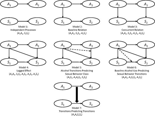
Graphical representations of ALTA Models 1–7. A₁ refers to alcohol use at time 1; A₂ refers to alcohol use at time 2; S₁ refers to sexual behavior at time 1; S₂ refers to sexual behavior at time 2. The loglinear notation for each model is shown below its graphical representation. Note that only the structural relations among variables are included in the graphical representations and loglinear notations. A latent class measurement model is assumed for each discrete latent variable.

The discussion of Models 1–3 focuses on the hypotheses expressed by the models and the probability restrictions required to fit these models. Odds ratios describing transitions in sexual behavior are not discussed for Models 1–3 because odds ratios involving P (S₂ = y|S₁ = x, A₁, A₂) are restricted to be equal across levels of A₁, and odds ratios involving P (S₂ = y|S₁ = x, A₁, A₂) are restricted to be equal across combinations of A₁ and A₂ for these models. The restrictions on the sets of probabilities of interest ensure that the odds ratios are also restricted.

The discussion of Models 4–6 focuses on the hypotheses expressed by the models and the odds ratio restrictions required to express them. Unlike Models 1–3, Models 4–6 cannot be expressed by probability restrictions alone. Probabilities describing transitions in sexual behavior are not discussed for these models because none of the probabilities are directly restricted to be equal to each other.³

Models Expressed by Probability Restrictions

The first three models considered hypothesize no or little association between between alcohol use and sexual behavior. To express Models 1–3, it is necessary to restrict sexual behavior latent class membership at time 1 and transition probabilities in sexual behavior to be equal across all alcohol use latent classes at time 1 (i.e., levels of A₁), as well as across all possible transitions in alcohol use latent classes from time 1 to time 2 (i.e., combinations of A₁ and A₂), in different ways. Each hypothesized model is fit using a different pattern of restrictions on three sets of probabilities of interest: (a) P (S₁ = x|A₁) (e.g., the probability of membership in the Monogamous latent class at time 1 conditional on membership in the Non-drinkers latent class at time 1); (b) P (S₂ = y|S₁ = x, A₁) (e.g., the probability of membership in the Multipartner Exposed latent class at time 2 conditional on membership in the Monogamous and Non-drinkers latent classes at time 1); (c) P (S₂ = y|S₁ = x, A₁,A₂) (e.g., the probability of membership in the Multipartner Exposed latent class at time 2 conditional on membership in the Binge Drinkers latent class at time 2 and the Monogamous and Non-drinkers latent classes at time 1).

Model 1

The independent processes model expresses the hypothesis that there is no association between alcohol use and sexual behavior at any time. In this model, alcohol use at baseline and transitions in alcohol use are not associated with sexual behavior at baseline or with transitions in sexual behavior. More specifically, the hypothesis that alcohol use and sexual behavior are unrelated implies that the probability of membership in the Monogamous latent class at time 1 is the same regardless of whether they were Non-drinkers, Experimental Drinkers or Binge Drinkers at time 1. It also implies that the probability of transitioning to Multipartner Exposed at time 2 for Monogamous individuals at time 1 is the same regardless of whether they transitioned from, for example, Non-drinking to Binge Drinking or remained Non-drinkers. This is the most restrictive model of the seven considered here.

The loglinear notation for this model is (A₁A₂, S₁S₂), implying that sexual behavior latent class membership at time 2 (S₂) is related to sexual behavior latent class membership at time 1 (S₁), but is independent of alcohol use latent class membership at time 1 (A₁) and alcohol use latent class membership at time 2 (A₂). The interactions between A₁ and A₂ and between S₁ and S₂ are illustrated graphically in Figure 1 by the solid arrows originating at A₁ and S₁ and terminating at A₂ and S₂, respectively. The absence of arrows connecting A₁ and A₂ to S₁ and S₂ in any way illustrates the absence of interactive effects between the processes, indicating that they are unrelated. As shown in Table 3, to express this model: (a) sexual behavior latent class membership probabilities at time 1 are restricted to be equal across alcohol use latent classes at time 1; (b) sexual behavior transition probabilities from time 1 to time 2 are restricted to be equal across alcohol use latent classes at time 1; (c) sexual behavior transition probabilities from time 1 to time 2 are restricted to be equal across transitions in alcohol use from time 1 to time 2.

Model 2

The baseline relation model expresses the hypothesis that there is a baseline association between alcohol use and sexual behavior, but that alcohol use at baseline and transitions in alcohol use are not associated with transitions in sexual behavior. Similar to the independent processes hypothesis, the baseline relation hypothesis implies that the probability of transitioning to Multipartner Exposed for Monogamous individuals is the same regardless of whether they transitioned from, for example, Non-drinking to Binge drinking or remained Non-drinkers. In contrast to the independent processes hypothesis, the baseline relation hypothesis implies that the probability of membership in the Monogamous latent class at time 1 may be different for Non-drinkers, Experimental Drinkers and Binge Drinkers at time 1.

The loglinear notation for this model is (A₁A₂,S₁S₂,A₁S₁), implying that A₁ latent class membership is related to S₁ latent class membership and that S₂ latent class membership is related to S₁ latent class membership, but that S₂ is conditionally independent of A₁ and A₂ given S₁. That is, for a given sexual behavior latent class at time 1, transitions in sexual behavior are unrelated to alcohol use. As shown in Figure 1, the additional baseline association between the processes hypothesized in this model is illustrated by the addition of a solid arrow originating at A₁ and terminating at S₁, which represents the additional interaction between A₁ and S₁ that distinguishes the baseline relation model from the independent processes model. As shown in Table 3, to express this model: (a) sexual behavior transition probabilities from time 1 to time 2 are restricted to be equal across alcohol use latent classes at time 1; (b) sexual behavior transition probabilities from time 1 to time 2 are restricted to be equal across transitions in alcohol use from time 1 to time 2.

Model 3

The concurrent relation model expresses the hypothesis that there are associations between alcohol use and sexual behavior at each time, but that transitions in alcohol use are not associated with transitions in sexual behavior. In contrast to the baseline relation hypothesis, the concurrent relation hypothesis implies that the probability of transitioning to Multipartner Exposed for Monogamous individuals may be different for Non-drinkers, Experimental Drinkers and Binge Drinkers at time 2. It also implies, however, that all time 2 Binge Drinkers have the same probability of making that transition in sexual behavior regardless of whether they were Non-drinkers, Experimental Drinkers or Binge Drinkers at time 1.

The loglinear notation for this model is (A₁A₂,S₁S₂,A₁S₁,A₂S₂), implying that A₁ latent class membership is related to S₁ latent class membership, and that S₂ latent class membership is related to S₁ and A₂ latent class membership, but that S₂ is conditionally independent of A₁ given S₁ and A₂. As shown in Figure 1, the additional time 2 association between the processes hypothesized in this model is illustrated by the addition of a solid arrow originating at A₂ and terminating at S₂, which represents the additional interaction between A₂ and S₂ that distinguishes the concurrent relation model from the independent processes model. As shown in Table 3, to express this model, sexual behavior transition probabilities from time 1 to time 2 are restricted to be equal across transitions in alcohol use from time 1 to time 2.

Models Expressed by Odds Ratio Restrictions

The next three models considered express more complex hypothesized associations between alcohol use and sexual behavior than those in Models 1–3. Models 4–6 differ in subtle ways that are not easily identified from the sets of probabilities discussed for Models 1–3. In Models 4–6, sexual behavior latent class membership and transition probabilities may vary across all alcohol use latent class memberships at time 1, and across all possible transitions in alcohol use from time 1 to time 2. To achieve the hypothesized models, restrictions are imposed on odds ratios rather than probabilities.

Model 4

The lagged effect model expresses the hypothesis that there is an association between alcohol use and sexual behavior at each time, and that there is an association between past (i.e., time 1) alcohol use and current (i.e., time 2) sexual behavior, but that transitions in alcohol use are not associated with transitions in sexual behavior. In contrast to the concurrent relation hypothesis, the lagged effect hypothesis implies that the probability of transitioning to Multipartner Exposed for Monogamous individuals may be different for each possible transition in alcohol use from time 1 to time 2. It also implies, however, that the odds ratio of transitioning to Multipartner Exposed in reference to Multipartner Safe at time 2 for Monogamous individuals compared to Daters at time 1 is the same for all types of alcohol use at time 1, and for all possible transitions in alcohol use from time 1 to time 2.

The loglinear notation for this model is (A₁A₂,S₁S₂,A₁S₁,A₂S₂,A₁S₂). As shown in Figure 1, the additional lagged association between time 1 alcohol use and time 2 sexual behavior hypothesized in this model is illustrated by the addition of a solid arrow originating at A₁ and terminating at S₂, which represents the additional interaction between A₁ and S₂ that distinguishes the lagged effect model from the concurrent relation model. As shown in Table 4, to express this model: (a) odds ratios describing transitions in alcohol use from time 1 to time 2 are restricted to be equal across sexual behavior latent class memberships at time 2; (b) odds ratios describing transitions in sexual behavior from time 1 to time 2 are restricted to be equal across alcohol use latent class memberships at time 1; (c) odds ratios describing transitions in sexual behavior are restricted to be equal across transitions in alcohol use from time 1 to time 2.

Model 5

The transitions predicting class model expresses the hypothesis that current and past alcohol use is associated with current sexual behavior, but combinations of past alcohol and sexual behavior are not associated with current sexual behavior. In this model, a direct effect of alcohol use transitions on sexual behavior latent class membership is hypothesized. That is, this model expresses the hypothesis that transitions in alcohol use, not the combination of alcohol use and sexual behavior at baseline, are associated with sexual behavior one year later. Similar to the lagged effect hypothesis, the transitions predicting class hypothesis implies that the odds ratio of transitioning to Multipartner Exposed in reference to Multipartner Safe for Monogamous indviduals compared to Daters is the same for all types of alcohol use at time 1, and for all possible transitions in alcohol use from time 1 to time 2. In contrast to the lagged effect hypothesis, the transitions predicting class hypothesis implies that odds ratios in other parts of the model may vary. That is, it implies that odds ratios describing transitions in alcohol use may vary across types of sexual behavior at time 2. For example, the change in odds of transitioning to Binge Drinking in relation to Non-drinking at time 2 for Experimental Drinkers compared to Non-drinkers at time 1 may vary across types of sexual behavior at time 2. Although these conditional odds ratios are not of particular interest here, restrictions on these odds ratios distinguish Model 4 from Model 5.

The loglinear notation for this model is (A₁S₁,A₁A₂S₂,S₁S₂). Remember that each element listed in the notation implies that nested lower-order effects are included in the model. For example, the term (A₁A₂S₂) implies that (A₁A₂), (A₁S₂), and (A₂S₂) are also modeled. The hypothesis that transitions in alcohol use are associated with sexual behavior is reflected in the three-way interaction term (A₁A₂S₂), which implies that the conditional association between A₁ and A₂ varies across levels of S₂. As shown in Figure 1, the additional association hypothesized in this model and specified by the three-way interaction term (A₁A₂S₂) is illustrated by the addition of a dotted arrow originating at A₁ and terminating at the solid arrow between A₂ and S₂. This convention indicates a three-way interaction among the latent class variable where the dotted arrow originates and the two latent class variables associated by the solid arrow where the dotted arrow terminates. As shown in Table 4, to express this model: (a) odds ratios describing transitions in sexual behavior from time 1 to time 2 are restricted to be equal across alcohol use latent class memberships at time 1; (b) odds ratios describing transitions in sexual behavior are restricted to be equal across transitions in alcohol use from time 1 to time 2.

Model 6

The baseline predicting transitions model expresses the hypothesis that combinations of past sexual behavior and alcohol use are associated with current sexual behavior. That is, a direct effect of the combination of time 1 alcohol use and sexual behavior on time 2 sexual behavior is hypothesized. Importantly, this model expresses the hypothesis that alcohol use at baseline, not transitions over time in alcohol use, is associated with transitions in sexual behavior over time. In contrast to the lagged effect hypothesis, the baseline predicting transitions hypothesis implies that the odds ratio of transitioning to Multipartner Exposed in reference to Multipartner Safe for Monogamous individuals compared to Daters may vary across types of alcohol use at time 1, but is the same across types of alcohol use at time 2. For example, Model 6 implies that all time 2 Non-drinkers, Experimental Drinkers and Binge Drinkers who were Non-drinkers at time 1 have the same odds ratio of transitioning to Multipartner Exposed in reference to Multipartner Safe for Monogamous individuals compared to Daters.

The loglinear notation for this model is (A₁A₂,A₁S₁S₂,A₂S₂). The hypothesis that combinations of past alcohol use and sexual behavior are associated with current sexual behavior is reflected in the three-way interaction term (A₁S₁S₂), which implies that the association between S₁ and S₂ is conditional on A₁. As shown in Figure 1, the additional association hypothesized in this model and specified by the three-way interaction term (A₁S₁S₂) is illustrated by the addition of a dotted arrow originating at A₁ and terminating at the solid arrow between S₁ and S₂. As shown in Table 4, to express this model: (a) odds ratios describing transitions in alcohol use from time 1 to time 2 are restricted to be equal across sexual behavior latent classes at time 2; (b) odds ratios describing transitions in sexual behavior are restricted to be equal across transitions in alcohol use from time 1 to time 2.

Model 7

is the unrestricted transitions predicting transitions or “full relation” model, which expresses the hypothesis that transitions in alcohol use are directly associated with transitions in sexual behavior. In this model, a direct effect of alcohol use transitions on sexual behavior transitions is hypothesized. This hypothesis implies that each type of alcohol use transition is associated with a different relative odds of each type of sexual behavior transition. That is, this hypothesis implies that the change in odds of transitioning to Multipartner Exposed in reference to Multipartner Safe for Monogamous individuals compared to Daters may vary for each possible transition in alcohol use over time.

This model is saturated in the structural model and the loglinear notation for this model is (A₁A₂S₁S₂). The hypothesis that combinations of alcohol use are associated with combinations of sexual behavior is reflected in the four-way interaction term (A₁A₂S₁S₂), which implies that the conditional association between S₁ and S₂ depends on the conditional association between A₁ and A₂. This model cannot be easily represented graphically using the conventions adopted for Models 1–6 because it would include solid arrows between each pair of latent class variables, and dotted arrows among all combinations of three latent class variables. In addition, it would have to include some representation of the four-way interaction. In Figure 1, a thicker solid arrow originating at the solid arrow representing the association between A₁ and A₂ and terminating at the solid arrow representing the association between S₁ and S₂ is meant to show that transitions in alcohol use are directly associated with transitions in sexual behavior. As shown in Tables 3 and 4, in order to express this model, no restrictions are placed on any probabilities or odds ratios in the structural model.

Nested Models

In the current article, the seven ALTA models described above are compared using the AIC and BIC. Alternatively, several of the models considered here are statistically nested and therefore may be compared using likelihood ratio tests. However, tests will often have a large number of degrees of freedom (df ) and it is unknown whether the distribution of the likelihood ratio test statistic follows a χ² distribution in those cases (Read & Cressie, 1988).⁴ In some applications, though, using the likelihood ratio test may be desirable. For reference, the relative nesting of Models 1–7 is indicated in Figure 2. A line between two models indicates that the lower numbered model is statistically nested within the higher numbered model, as well as all other models within which the higher numbered model is itself nested. For example, Model 4 is nested within Models 5, 6, and 7, but Model 5 is nested only within Model 7.

Figure 2.

Relative nesting of ALTA Models 1–7. A line between two models indicates that the lower numbered model is statistically nested within the higher numbered model, as well as all other models within which the higher numbered model is itself nested.

Study II: Modeling the Link Between Alcohol Use and Sexual Behavior

Participants and Measures

Participants and measures were the same as those in Study I.

Analysis

The association between development in alcohol use and development in sexual behavior was examined by fitting the seven ALTA models described above. The models were compared using the AIC and BIC to determine which provided the optimal balance of fit and parsimony in its description of the association between sexual behavior and alcohol use over time.

Software

ℓEM (Vermunt, 1997a,b) was used for fitting the models described. ℓEM is a program for categorical data analysis that can be used to analyze nominal, ordinal and interval level discrete data. Among other types of models, it may be used to estimate loglinear models, latent structure models for categorical items, and LISREL-like models for categorical endogenous variables. That is, ℓEM can be used for LCA, LTA and ALTA. ℓEM provides maximum likelihood estimates for model parameters using an Expectation-Maximization (EM) algorithm. Several other software options exist for fitting certain ALTA models, including Mplus (Muthén & Muthén, 1998–2007), and software available from Flaherty (2008a,b). These options are discussed in more detail in the Discussion. ℓEM syntax used to fit Models 1–7 is included in the Appendix.

Results

Fit statistics for Models 1–7 are shown in Table 5. Model 3 had the lowest AIC and BIC values, and was selected as providing the optimal balance of fit and parsimony in its description of the association between development in alcohol use and development in sexual behavior. The selection of Model 3 suggested that: (a) alcohol use and sexual behavior were associated at each time, and (b) given particular transitions in alcohol use from time 1 to time 2, a particular transition in sexual behavior from time 1 to time 2 was not associated with alcohol use at time 1. For example, this means that the probability of transitioning from the Daters latent class to the Multipartner Safe latent class was the same for those who: (a) transitioned from Non-drinking to Binge drinking, (b) transitioned from Experimental Drinking to Binge Drinking, and (c) continued to Binge Drink over time. Importantly, this means that knowing about time 1 to time 2 alcohol use transitions did not add to the ability to predict transitions to risky sexual behavior.

Table 5.

Fit Statistics for Associative Latent Transition (ALTA) Models

	Log-likelihood	df	AIC	BIC
Model 1	−14597.786	82872	29337.571	29743.756
Model 2	−14396.601	82864	28951.202	29403.154
Model 3	−14336.975	82856	28847.950	29345.669
Model 4	−14331.220	82848	28852.441	29395.927
Model 5	−14311.405	82816	28876.810	29603.365
Model 6	−14317.085	82832	28856.169	29491.190
Model 7	−14222.609	82680	28971.217	30475.815

Note: Boldface type indicates selected model.

Of particular interest were the transitions from the Daters and Monogamous latent classes to the Multipartner Safe and Multipartner Exposed latent classes. Transition probabilities from the Daters and Monogamous latent classes to the Multipartner Safe and Multipartner Exposed latent classes by time 2 alcohol use are shown in Table 6. The sexual behavior transition probabilities are the same for time 1 Non-drinkers, Experimental Drinkers and Binge Drinkers (i.e., regardless of time 1 alcohol use latent class membership). The probabilities in the table are the probabilities of sexual behavior latent class membership at time 2 conditional on sexual behavior latent class membership at time 1 and alcohol use latent class membership at times 1 and 2.⁵ Alcohol use latent class membership at time 1 is not included as a column in Table 6 because the probabilities are the same regardless of alcohol use at time 1.

Table 6.

Selected Time 1 to Time 2 Transition Probabilities in Sexual Behavior by Time 2 Alcohol Use for Time 1 Non-drinkers, Experimental Drinkers and Binge Drinkers

Time 1	Time 2	Time 2 Sexual Behavior
Sexual Behavior	Alcohol Use	M-P Safe	M-P Exposed
Daters	Non-drinkers	0.111	0.036
	Experimenters	0.092	0.087
	Binge Drinkers	0.109	0.137
Monogamous	Non-drinkers	0.101	0.076
	Experimenters	0.070	0.151
	Binge Drinkers	0.088	0.255

Note: M-P Safe is Multipartner Safe; M-P Exposed is Multipartner Exposed. These data correspond to an odds ratio of 2.3; this odds ratio is the same for all types of Time 1 Alcohol Use and for all transitions in Alcohol Use from Time 1 to Time 2.

A close examination of Table 6 reveals interesting associations between alcohol use and sexual behavior. Daters and Monogamous individuals at time 1 who were Non-drinkers at time 2 were more likely to transition to the Multipartner Safe latent class than the Multipartner Exposed latent class at time 2. For example, time 1 Daters who were time 2 Non-drinkers had an 11.1% chance of transitioning to the Multipartner Safe latent class compared to a 3.6% chance of transitioning to the Multipartner Exposed latent class at time 2. In addition, time 1 Monogamous individuals who were time 2 Binge Drinkers were at highest risk for transitioning to the Multipartner Exposed latent class at time 2. That is, 25.5% of time 1 Monogamous individuals who were time 2 Binge Drinkers transitioned to the Multipartner Exposed latent class at time 2.

In general, Table 6 suggests that individuals with less risky alcohol use at time 2 were more likely to transition to Multipartner Safe sexual behavior compared to Multipartner Exposed sexual behavior at time 2. The results also suggest that, in general, individuals with more risky alcohol use at time 2 were more likely to transition to Multipartner Exposed sexual behavior compared to Multipartner Safe sexual behavior at time 2, and that Monogamous individuals at time 1 who were most risky in their alcohol use at time 2 were at highest risk for transitioning to the most risky sexual behavior latent class.

As discussed earlier, Model 3 specified that the odds ratio for transitioning to the Multipartner Exposed latent class in reference to the Multipartner Safe latent class (i.e., transitioning to high-risk compared to low-risk) from the Monogamous latent class compared to from the Daters latent class (i.e., from low-risk compared to from even lower-risk) was the same for all types of alcohol use at time 1, and for all transitions in alcohol use from time 1 to time 2. The odds ratio was estimated at 2.3. This means that the odds of membership in the Multipartner Exposed latent class at time 2 (in reference to the Multipartner Safe latent class) were approximately 2 times higher for time 1 Monogamous individuals compared to Daters, regardless of transitions in alcohol use from time 1 to time 2.

Discussion

The purpose of this article was to present a flexible approach to ALTA based on the general framework of loglinear modeling with latent variables. ALTA provides a way to model the structural relations between two discrete developmental processes simultaneously over time. To motivate the application of ALTA, the association between alcohol use development and sexual behavior development was examined in two studies.

In Study I, development in alcohol use and sexual behavior were modeled separately. Latent classes of alcohol use and sexual behavior were identified, and change over time in class membership was described for each process. In Study II, seven ALTA models expressing alternative hypotheses about the association between alcohol use and sexual behavior were discussed in detail. The seven models were fit to data and compared, and the selected model was used to make conclusions about the nature of the association between alcohol use and sexual behavior development. Results showed the two processes were associated at both times, but that transitions in sexual behavior did not depend on transitions in alcohol use.

Model Specification in ALTA

Many ALTA models differ in subtle ways that are easy to overlook during model specification, as well as when viewing the results. This is partly because some models imply differences in probabilities, and others in odds ratios. A seemingly small misspecification in an ALTA model may result in the expression of a hypothesis that differs substantially from the intended hypothesis. The primary goal of the current article was to illuminate subtle differences in model specification in ALTA, and to provide information on how to fit these models precisely. Subtle differences in specification can result in scientifically important differences in interpretation.

To fit these models precisely, it is important to be able to consider both probabilities and odds ratios. Three of the models considered here (Models 4–6) cannot be expressed by considering only probabilities. The approach discussed here is based on loglinear modeling with latent variables. In this approach, associations and interactions between the processes are added to the model as interactive effects. Models 4–6 differ only in their odds ratio restrictions, which are specified by the inclusion/exclusion of different interactive effects in the models. The presence of effects was shown in the loglinear notations of the models, and was illustrated in the graphical representations of the models in Figure 1 using solid and dotted arrows. When effects are added, restrictions are removed.

Consider Models 4 and 6. The differences in the hypotheses expressed by these two models may have important implications for the implementation of prevention programs for STIs. The hypothesis expressed by Model 6 includes a direct effect of combinations of past alcohol use and sexual behavior on transitions in sexual behavior, whereas the hypothesis expressed by Model 4 does not. It is impossible to distinguish these two models if only probabilities are considered. To distinguish these two models, odds ratios describing transitions in sexual behavior from time 1 to time 2 must be free to vary across levels of alcohol use at time 1 in Model 6 but not in Model 4, and all probabilities must be free to vary. It is possible to do this when taking a loglinear modeling approach to ALTA.

Comparison with Previous ALTA Work

Previous ALTA work (Flaherty, 2008a,b; Witkiewitz & Villarroel, 2009) used a specific parameterization of the ALTA model based solely on probabilities, and considered models expressed by probability restrictions. The models discussed by Flaherty (2008b) fit into the general framework discussed here. In Flaherty's work, the independence model corresponds to the independent processes model (Model 1), the cross-sectional association model corresponds to the baseline relation model (Model 2), and the full association model corresponds to the transitions predicting transitions model (Model 7). The full association model does not include any parameter restrictions on the probabilities that are used to define the ALTA models considered by Flaherty (2008a,b). That is, the full association model is the (structurally) saturated model for a model with four discrete latent variables, which corresponds to (A₁A₂S₁S₂) in the current article. Models 3–6 discussed here do not appear in Flaherty's work and are scientifically important “intermediate” models between the cross-sectional and full association models.

The longitudinal association model in Flaherty's work is not considered in the current article because it is a non-hierarchical loglinear model. Non-hierarchical loglinear models that do not include all lower-order effects when higher order effects are included in the model are rarely used in practice. In the context of the discussion presented here, Flaherty's longitudinal association model omits the A₁S₁ interaction from the (structurally) saturated model. In the longitudinal association model, the patterns of restrictions on the probabilities and odds ratios of interest would be the same as those in Model 7 (i.e., no patterns of restrictions) due to the inclusion of the four-way interaction term specified by no parameter restrictions on the η parameters in the ALTA models considered by Flaherty (2008a,b). The current article considers only hierarchical models because they correspond to the hypothesized associations between alcohol use and sexual behavior. See Rindskopf (1990) for a discussion of non-hierarchical and other non-standard loglinear models in the social sciences.

In addition, previous ALTA work used nested G² difference tests to select a final model for interpretation. When there are a large number of df for these tests, the distribution of the test statistic is unknown (Read & Cressie, 1988). Penalized criteria like the AIC and BIC may be more helpful for model comparison and selection with large, sparse contingency tables. Here, the AIC and BIC were used for model selection.

Association Versus Causality

ALTA models, as they are presented and discussed here, do not provide conclusions about causal effects between alcohol use and sexual behavior. Neither alcohol use nor sexual behavior were experimentally manipulated, and the decision to model alcohol use predicting sexual behavior was made to facilitate a particular interpretation in the relation between the two processes. The predictor and predicted processes could be switched, so that the arrows in Figure 1 originate at sexual behavior and terminate at alcohol use. When the processes are switched, the fit statistics for Models 1, 2, 3 and 7 are unchanged. The fit statistics for Models 4, 5, and 6, however, are different because different effects are included in the models, and the hypotheses expressed by the models are different. Decisions about which process is considered the predictor, and which the predicted, should be based on theory and the particular research questions at hand.

Limitations

ALTA provides a promising approach to researchers interested in studying the development of two multidimensional latent variables simultaneously over time. There are, however, limitations to the method that researchers may wish to consider before applying it to address substantive research questions.

Model Estimation and Identification

Large numbers of parameters are estimated with ALTA. A large sample size is highly recommended when fitting these models to help avoid model estimation and identification problems. In addition, because of the large number of parameters estimated, some models may take a very long time to run in certain software packages, especially when there are missing data.

An issue that may often contribute to model estimation and identification challenges is model dimensionality. The size of the contingency tables on which ALTA is based are extremely large and are likely to be extremely sparse. Sparseness can make model estimation and maximum likelihood solution identification difficult. This issue increases exponentially as the number of items, number of response categories per item, and/or the number of times is increased. This is an important consideration when developing the latent class and latent transition models that will be combined in ALTA.

Statistical Power

Little is known about statistical power in latent class models. However, one factor that is known to contribute to the power of hypothesis tests in LCA and LTA is the strength of the measurement model. High homogeneity within latent classes, high latent class separation, and item-response probabilities close to 0 and 1 increase the strength of the measurement model (Collins & Lanza, in press). Although it was not the focus of the current article, the importance of measurement models in ALTA cannot be overstated. During the model building process for ALTA, it is important to carefully consider, examine and evaluate the measurement models of all latent class variables with LCA and LTA prior to fitting models with ALTA.

In addition, in the approach presented in the current article, interactive effects are added as models become more complex, in order to allow for a variety of associations and interactions between the processes over time. For example, fitting the transitions predicting transitions model requires a four-way interaction. It is important to consider that a great deal of power is likely necessary to detect a four-way interaction. It may be important for researchers to consider hypothesizing associations between processes that correspond to “intermediate” models between the baseline relation and transitions predicting transitions models (e.g., Models 3–6) in part because power to detect the need for multi-way interactions may be limited and the estimation of models with large numbers of unnecessary parameters may be unstable. Exploring the strength of the relation between the two processes required to provide enough power to detect the need for higher-order interactions in ALTA models is an area where more work is needed.

Software

There are several software options available for ALTA, including ℓEM, Mplus and software available from Flaherty (2008b). Flaherty's software requires the use of parameter restrictions on probabilities to fit models that are nested within the full association model (i.e., Model 7). Mplus is well-known and may be used to fit a variety of latent class, latent transition and ALTA models. To the best of our knowledge, currently, Mplus may not be used to fit the transitions predicting transitions model (Model 7) because it can handle at most three-way interactions in loglinear models with latent variables. ℓEM is designed specifically for categorical variables. Model specification in ℓEM is straightforward, as it simply requires the loglinear shorthand notation used here. Model specification in Mplus is more difficult, as is model specification in Flaherty's software, especially when parameter restrictions must be used to specify models other than the full association model.

Extensions of ALTA

The current article limits its discussion to ALTA that models development in two discrete latent variables over time. This was to focus on the substantive and statistical features of the models. Possible extensions to this model are numerous and include the addition of grouping variables or covariates, the inclusion of three or more processes, and linking a LTA to other types of models like a latent growth curve model.

Conclusions

ALTA is a promising approach to modeling two or more discrete, multidimensional latent variables simultaneously over time. Taking a loglinear modeling perspective on ALTA provides a flexible approach that enables fitting a broad array of models, which opens up possibilities for testing hypotheses about growth and change. Using advanced statistical methods like ALTA to examine the development of one process in the context of other developmental processes may provide a better understanding of all processes.

Appendix

ℓEM Syntax for Models 1–7

All associative latent transition models were estimated using ℓEM (Vermunt, 1997a,b). ℓEM and the accompanying user's guide are available by free download from the University of Tilburg's website at http://www.uvt.nl/faculteiten/fsw/organisatie/departementen/mto/software2.html.

Model notes and labels used in ℓEM syntax

• Five latent classes of sexual behavior: X = Time 1 sexual behavior; Y = Time 2 sexual behavior; A = Number of past-year dating partners at time 1; B = Past-year sex at time 1; C = Number of past-year sexual partners at time 1; D= Past-year exposure to STIs at time 1; E = Number of past-year dating partners at time 2; F = Past-year sex at time 2; G = Number of past-year sexual partners at time 2; H = Past-year exposure to STIs at time 2

• Three latent classes of alcohol use: U = Time 1 alcohol use; V = Time 2 alcohol use; M = Past-year alcohol use at time 1; N = Past-month alcohol use at time 1; O = Past-month binge drinking at time 1; P = Past-year alcohol use at time 2; Q = Past-month alcohol use at time 2; R = Past-month binge drinking at time 2

ℓEM syntax:

1. Full syntax for Model 1: Independent Processes

*ALTA - INDEPENDENT PROCESSES
*2 TIMES
*NO MISSING DATA
lat	4			*number of latent variables
man	14		*number of manifest items
dim	5	5
	3	3
	3	3
	2	2
	3	3
	2	2
	2	2
	2	2
	2	2	*dimension of each latent variable and item
lab	X	Y
	U	V
	A	E
	B	F
	C	G
	D	H
	M	P
	N	Q
	O	R	*label of each latent variable and item
mod	XYUA		{XY	,UV
	A|X		B|X		C|X	D|X
	M|U		N|U		O|U
	E|Y		eq1	A|X
	F|Y		eq1	B|X
	G|Y		eq1	C|X
	H|Y		eq1	D|X
	P|V		eq1	M|U
	Q|V		eq1	N|U
	R|V		eql	O|U			*specify model
rec	2255						*data file contains 2255 records
cri	.0000000000000001					L	*change convergence criterion
sta	A|X		[.76	.16	.08 0		.20	.80	.07	.58	.35	.04	.03	.92	.03	.04	.93]
sta	B|X		[ 1	0		1	0		0	1		0	1		0	1]
sta	C|X		[ 1	0	0	1	0	0	0	.99	.01	0	.38	.62	0	.09	.91]
sta	D|X		[ 1	0		1	0		.45	.55		1	0		.28	.72]
sta	M|U		[.94	.06	0		1		0		1]
sta	N|U		[ 1	0	1		0		.13		.87]
sta	O|U		[ 1	0	.47	.53	0	1]		*starting values
nfr										*suppress frequencies in output
nR2										*suppress R2 measures in output
npa										*suppress loglinear parameters in output
wco est_prob_model_1.dat										*write probability estimates to a dataset
dat lemdata_alta_nomiss 2t.txt										*data file

2. Modification of the “model” statement for Model 2: Baseline Relation

mod	XYUA	{XY	,UV	,XU}
	A|X	B|X	C|X	D|X
	M|U	N|U	O|U
	E|Y	eq1	A|X
	F|Y	eq1	B|X
	G|Y	eq1	C|X
	H|Y	eq1	D|X
	P|V	eq1	M|U
	Q|V	eq1	N|U
	R|V	eql	O|U		*specify model

3. Modification of the “model” statement for Model 3: Concurrent Relation

mod	XYUA	{XY	,UV	,XU	,YV}
	A|X	B|X	C|X	D|X
	M|U	N|U	O|U
	E|Y	eq1	A|X
	F|Y	eq1	B|X
	G|Y	eq1	C|X
	H|Y	eq1	D|X
	P|V	eq1	M|U
	Q|V	eq1	N|U
	R|V	eql	O|U		*specify model

4. Modification of the “model” statement for Model 4: Lagged Effect

mod	XYUV	{XY	,UV	,XU	,YV	,UY}
	A|X	B|X	C|X	D|X
	M|U	N|U	O|U
	E|Y	eq1	A|X
	F|Y	eq1	B|X
	G|Y	eq1	C|X
	H|Y	eq1	D|X
	P|V	eq1	M|U
	Q|V	eq1	N|U
	R|V	eql	O|U			*specify model

5. Modification of the “model” statement for Model 5: Alcohol Transitions Predicting Sexual Behavior Class

mod	XYUV	{XY	,XU	,UYV}
	A|X	B|X	C|X	D|X
	M|U	N|U	O|U
	E|Y	eq1	A|X
	F|Y	eq1	B|X
	G|Y	eq1	C|X
	H|Y	eq1	D|X
	P|V	eq1	M|U
	Q|V	eq1	N|U
	R|V	eql	O|U		*specify model

6. Modification of the “model” statement for Model 6: Baseline Alcohol Use Predicting Sexual Behavior Transitions

mod	XYUV	{XUY	,UV	,YV}
	A|X	B|X	C|X	D|X
	M|U	N|U	O|U
	E|Y	eq1	A|X
	F|Y	eq1	B|X
	G|Y	eq1	C|X
	H|Y	eq1	D|X
	P|V	eq1	M|U
	Q|V	eq1	N|U
	R|V	eql	O|U		*specify model

7. Modification of the “model” statement for Model 7: Transitions Predicting Transitions (Full Relation)

mod	XYUV
	A|X	B|X	C|X	D|X
	M|U	N|U	O|U
	E|Y	eq1	A|X
	F|Y	eq1	B|X
	G|Y	eq1	C|X
	H|Y	eq1	D|X
	P|V	eq1	M|U
	Q|V	eq1	N|U
	R|V	eql	O|U		*specify model

References

- Agresti A. Categorical data analysis. Wiley-Interscience; Hoboken, NJ: 2002. Loglinear models for contingency tables. (chap. 8) [Google Scholar]
- Akaike H. A new look at the statistical model identification. IEEE Transactions on Automatic Control. 1974;19:716–723. [Google Scholar]
- Beadnell B, Morrison DM, Wilsdon A, Wells EA, Murowchick E, Hoppe M, et al. Condom use, frequency of sex, and number of partners: Multidimensional characterization of adolescent sexual risk-taking. The Journal of Sex Research. 2005;42:192–202. doi: 10.1080/00224490509552274. [DOI] [PubMed] [Google Scholar]
- Biemer PP, Wiesen C. Measurement error evaluation of self-reported drug use: A latent class analysis of the US National Household Survey on Drug Abuse. Journal of the Royal Statistical Society, Series A (Statistics in Society) 2002;165(1):97–119. [Google Scholar]
- Bishop YMM, Fienberg SE, Holland PW. Discrete multivariate analysis: Theory and practice. The MIT Press; Cambridge, MA: 1975. [Google Scholar]
- Bollen KA, Curran PJ. Latent curve models: A structural equation perspective. Wiley; Hoboken, NJ: 2006. [Google Scholar]
- Bureau of Labor Statistics, U.S. Department of Labor . National Longitudinal Survey of Youth 1997 cohort, 1997–2006 (rounds 1–9) [Data file] The Ohio State University; Columbus, OH: 2007. Produced by the National Opinion Research Center, the University of Chicago and distributed by the Center for Human Resource Research. [Google Scholar]
- Chung H, Flaherty BP, Schafer JL. Latent class logistic regression: Application to marijuana use and attitudes among high school seniors. Journal of the Royal Statistical Society, Series A. 2006;169(Part 4):723–743. [Google Scholar]
- Chung H, Park Y, Lanza ST. Latent transition analysis with covariates: Pubertal timing and substance use behaviors in adolescent females. Statistics in Medicine. 2005;24:2895–2910. doi: 10.1002/sim.2148. [DOI] [PubMed] [Google Scholar]
- Clogg CC. Latent class models. In: Arminger G, Clogg CC, Sobel ME, editors. Handbook of statistical modeling for the social and behavioral sciences. Plenum Press; New York, NY: 1995. pp. 311–359. [Google Scholar]
- Collins LM, Graham JW, Rousculp SS, Hansen WB. Heavy caffeine use and the beginning of the substance use onset process: An illustration of latent transition analysis. In: Bryant K, Windle M, West S, editors. The science of prevention: Methodological advances fromalcohol and substance abuse research. American Psychological Association; Washington, D.C.: 1997. pp. 79–99. [Google Scholar]
- Collins LM, Lanza ST. Latent class and latent transition analysis for applications in the social, behavioral and health sciences. Wiley; New York: in press. [Google Scholar]
- Collins LM, Wugalter SE. Latent class models for stage-sequential dynamic latent variables. Multivariate Behavioral Research. 1992;27:131–157. [Google Scholar]
- Everitt BS, Dunn G. Log-linear modeling, latent class analysis, or correspondence analysis: Which method should be used for the analysis of categorical data? In: Langeheine R, Rost J, editors. Latent trait and latent class models. Plenum Press; New York, NY: 1988. pp. 109–128. [Google Scholar]
- Flaherty BP. Examining contingent discrete change over time with associative latent transition analysis. In: Hancock GR, Samuelsen KM, editors. Advances in latent variable mixture models. Information Age Publishing, Inc; Charlotte, NC: 2008a. pp. 77–103. [Google Scholar]
- Flaherty BP. Testing the degree of cross-sectional and longitudinal dependence between two discrete dynamic processes. Developmental Psychology. 2008b;44(2):468–480. doi: 10.1037/0012-1649.44.2.468. [DOI] [PMC free article] [PubMed] [Google Scholar]
- Goodman LA. Exploratory latent structure analysis using both identifiable and unidentifiable models. Biometrika. 1974;61:215–231. [Google Scholar]
- Guo J, Collins LM, Hill KG, Hawkins JD. Developmental pathways to alcohol abuse and dependence in young adulthood. Journal of Studies on Alcohol. 2000;61:799–808. doi: 10.15288/jsa.2000.61.799. [DOI] [PMC free article] [PubMed] [Google Scholar]
- Hagenaars JA. LCAG - loglinear modelling with latent variables: A modified LISREL approach. In: Saris WE, Gallhofer IN, editors. Sociometric research: Data analysis. Vol. 2. Macmillian; London: 1988. [Google Scholar]
- Hagenaars JA. Exemplifying longitudinal loglinear analysis with latent variables. In: Van der Heijden PGM, Jansen W, Francis B, Seeber GUH, editors. Statistical modelling. Elsevier; Amsterdam: 1992. [Google Scholar]
- Hagenaars JA. Loglinear models with latent variables. Sage Publications; Newbury Park: 1993. No. 07–094. [Google Scholar]
- Hagenaars JA. Latent variables in log-linear models of repeated observations. In: von Eye A, Clogg CC, editors. Latent variables analysis: Applications for developmental research. Sage Publications; Thousand Oaks, CA: 1994. pp. 329–352. [Google Scholar]
- Heinen T. Latent class and discrete latent trait models: Similarities and differences. Sage Publications; Thousand Oaks, CA: 1996. Log-linear models and latent class analysis; pp. 30–64. [Google Scholar]
- Lanza ST, Collins LM. A new SAS procedure for latent transition analysis: The development of dating and sexual risk behavior. Developmental Psychology. 2008;44(2):446–456. doi: 10.1037/0012-1649.44.2.446. [DOI] [PMC free article] [PubMed] [Google Scholar]
- Lanza ST, Collins LM, Lemmon D. PROC LCA: A SAS procedure for latent class analysis. Structural Equation Modeling. 2007;14(4):671–694. doi: 10.1080/10705510701575602. [DOI] [PMC free article] [PubMed] [Google Scholar]
- Lanza ST, Collins LM, Schafer JL, Flaherty BP. Using data augmentation to obtain standard errors and conduct hypothesis tests in latent class and latent transition analysis. Psychological Methods. 2005;10:84–100. doi: 10.1037/1082-989X.10.1.84. [DOI] [PubMed] [Google Scholar]
- Lanza ST, Flaherty BP, Collins LM. Latent class and latent transition analysis. In: Schinka JA, Velicer WF, editors. Handbook of psychology: Vol. 2, research methods in psychology. Wiley; Hoboken, NJ: 2003. pp. 663–685. [Google Scholar]
- Lazarsfeld PF, Henry NW. Latent structure analysis. Houghton Mifflin; Boston, MA: 1968. [Google Scholar]
- Monga N, Rehm J, Fischer B, Brissette S, Bruneau J, El-Guebaly N, et al. Using latent class analysis (LCA) to analyze patterns of drug use in a population of illegal opioid users. Drug and Alcohol Dependence. 2007;88(1):1–8. doi: 10.1016/j.drugalcdep.2006.08.029. [DOI] [PubMed] [Google Scholar]
- Muthén LK, Muthén BO. M plus user's guide. Fifth ed. Muthén & Muthén; Los Angeles, CA: 1998–2007. [Google Scholar]
- Nagin DS. Group-based modeling of development. Harvard University Press; Cambridge, MA: 2005. [Google Scholar]
- Newman PA, Zimmerman MA. Gender differences in HIV-related sexual risk behavior among urban African American youth: A multivariate approach. AIDS Education and Prevention. 2000;12:308–325. [PubMed] [Google Scholar]
- Read TRC, Cressie NAC. Goodness-of-fit statistics for discrete multivariate data. Springer-Verlag; New York, NY: 1988. [Google Scholar]
- Reboussin BA, Song E-Y, Shrestha A, Lohman KK, Wolfson M. A latent class analysis of underage problem drinking: Evidence from a community sample of 16–20 year olds. Drug and Alcohol Dependence. 2006;83(3):199–209. doi: 10.1016/j.drugalcdep.2005.11.013. [DOI] [PMC free article] [PubMed] [Google Scholar]
- Rindskopf D. Non-standard log-linear models. Psychological Bulletin. 1990;108(1):150–162. [Google Scholar]
- Schwartz G. Estimating the dimension of a model. Annals of Statistics. 1978;6:461–464. [Google Scholar]
- Vermunt JK. Causal log-linear modeling with latent variables and missing data. In: Engel U, Reinecke J, editors. Analysis of change: Advanced techniques in panel data analysis. Walter de Gruyter; Berlin/New York: 1996. pp. 35–60. [Google Scholar]
- Vermunt JK. LEM: A general program for the analysis of categorical data. Department of Methodology and Statistics, Tilburg University; 1997a. [Google Scholar]
- Vermunt JK. Log-linear models for event histories. Sage Publications; Thousand Oakes, CA: 1997b. [Google Scholar]
- Whitesell NR, Beals J, Mitchell CM, Novins DK, Spicer P, Manson SM, et al. Latent class analysis of substance use: Comparison of two American Indian reservation populations and a national sample. Journal of Studies on Alcohol and Drugs. 2006;67(1):32–43. doi: 10.15288/jsa.2006.67.32. [DOI] [PubMed] [Google Scholar]
- Willett JB, Sayer AG. Cross-domain analyses of change over time: Combining growth modeling and covariance structure analysis. In: Marcoulides GA, Schumacker RE, editors. Advanced structural equation modeling. Erlbaum; Mahwah, NJ: 1996. pp. 125–157. [Google Scholar]
- Witkiewitz K, Villarroel NA. Dynamic association between alcohol lapses and negative affect following alcohol treatment. Journal of Consulting and Clinical Psychology. 2009;77(4):633–644. doi: 10.1037/a0015647. [DOI] [PMC free article] [PubMed] [Google Scholar]