Superordinate shape classification using natural shape statistics

Abstract

This paper investigates the classification of shapes into broad natural categories such as animal or leaf. We asked whether such coarse classifications can be achieved by a simple statistical classification of the shape skeleton. We surveyed databases of natural shapes, extracting shape skeletons and tabulating their parameters within each class, seeking shape statistics that effectively discriminated the classes. We conducted two experiments in which human subjects were asked to classify novel shapes into the same natural classes. We compared subjects’ classifications to those of a naive Bayesian classifier based on the natural shape statistics, and found good agreement. We conclude that human superordinate shape classifications can be well understood as involving a simple statistical classification of the shape skeleton that has been “tuned” to the natural statistics of shape.

Introduction

Most contemporary approaches to object recognition involve matching shapes to a simple database of stored object models. But human conceptual structures have long been thought to be hierarchical (Rosch, 1973), meaning they contain highly specific (subordinate) and highly abstracted (superordinate) object categories. Indeed, from a computational point of view, a hierarchical matching procedure, in which objects are indexed into broad categories first before increasingly fine classifications are made, is well-known to greatly increase matching efficiency (Quinlan & Rivest, 1989). Richards and Bobick (1988) have argued that an initial rough classification of sensory stimuli into coarse semantic classes (animal, vegetable or mineral?) serves as an effective entry point into a natural ontology, allowing rapid use of perceptual information to guide meaningful responses. In this paper we ask whether such an initial classification in the realm of shape can be effected using a very small set of shape parameters if (a) the parameters are well chosen, and (b) the classification is informed by knowledge of the way these parameters are distributed in the real world.

Superordinate classification is an inherently difficult problem, because objects within a broader class generally differ from each other in a larger variety of ways than do those within a narrower class (Rosch, Mervis, Gray, Johnson, & Boyes-Braem, 1976). Recent studies have shown that human subjects can accurately place images into natural categories (e.g. does the image contain an animal?) after exposures as brief as 20msec, with classification essentially complete by 150msec of processing (Thorpe, Fize, & Marlot, 1996; VanRullen & Thorpe, 2001). The rapidity of this classification has been taken to suggest an entirely feed-forward architecture lacking recurrent or iterative computation (Serre, Oliva, & Poggio, 2007). These studies generally involve a very nonspecific kind of natural image classification—the stimuli may contain a variety of objects and a multiplicity of cues, including shape, color, texture, etc.—both within target objects (if any are present) as well as elsewhere in the image. By contrast our focus is on shape properties specifically, and their utility in classifying individual objects. Hence while our task is broadly similar in that it involves a natural classification, our stimuli consist of a single, isolated object—a black silhouette presented on a white background, without additional features or context—with the focus being on the nature of the shape properties that subjects use to classify the shape.

Parameterizations of shape

Shape can be represented over a virtually infinite variety of parameters, including Fourier descriptors (Chellappa & Bagdazian, 1984), boundary moments (Sonka, Hlavac, & Boyle, 1993; Gonzalez & Woods, 1992), chain codes (Freeman, 1961), geons (Biederman, 1987), codons (Richards, Dawson, & Whittington, 1988), shape grammars (Fu, 1974; Leyton, 1988), shape matrices (Goshtasby, 1985), the convex hull-deficiency (Sonka et al., 1993; Gonzalez & Woods, 1992), and medial axes (Blum, 1973; Blum & Nagel, 1978). Each of these choices has arguments in its favor, and contexts in which they have proved useful (see Zhang & Lu, 2004 for a review). But so far none have been quantitatively validated with respect to ecological shape categories, meaning that their respective benefits have not been tied concretely to the statistical patterns that prevail among natural shapes. In this paper we focus on skeletal (medial axis) representations, which were actually originally conceived by Blum (1973) as a method for effectively describing and distinguishing biological forms. Effective representation of global part structure is especially essential for distinguishing natural classes because it tends to vary between phylogenetic categories.

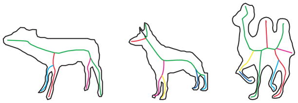
Human representation of natural shapes has long been thought to depend heavily on part structure (Barenholtz & Feldman, 2003; Biederman, 1987; de Winter & Wagemans, 2006; Hoffman & Richards, 1984; Hoffman & Singh, 1997; Marr & Nishihara, 1978), and a number of studies have established the psychological reality of medial axis representations (Harrison & Feldman, 2009; Psotka, 1978; Kovacs & Julesz, 1994; Kovacs, Feher, & Julesz, 1998). Modern approaches to medial axis computation are plentiful (Brady & Asada, 1984; Katz & Pizer, 2003; Kimia, 2003; Siddiqi, Shokoufandeh, Dickinson, & Zucker, 1999; Zhu, 1999), though many still suffer from the presence of pervasive spurious axes, which in most methods tend to arise whenever there is noise along the contour. Spurious axes are a key obstacle to achieving meaningful distinctions among shape categories, because they spoil what would otherwise be the desired isomorphism between axes and parts; that is, spurious axes do not correspond to parts that are either psychologically real or physically meaningful. To minimize the problem of spurious axes we use the framework introduced in Feldman and Singh (2006) for estimating the shape skeleton. Briefly, the main idea in this approach is to treat the shape as data and try to “explain it” as the result of a stochastic process of growth emanating from a skeletal structure. A prior over skeletons is defined, which determines which skeletons are considered more plausible in general, independent of the particular shape at hand. The prior tends to favor simple skeletons, meaning those with fewer and/or less curved branches. The likelihood function defines the probability of the shape at hand conditioned on a hypothetical skeleton, and thus serves as a stochastic model of shape generation. The goal is then to estimate the skeleton that maximizes the posterior, meaning the one that has the best combination of prior plausibility with fit to the shape; this skeleton, called the maximum a posteriori or MAP skeleton, is the skeleton that “best explains” the shape (see examples in Fig. 1). A more technical explanation of Bayesian skeleton estimation is given in the Appendix. Critically for our purposes, the MAP skeleton tends to recover the qualitative part structure of the shape, with one distinct skeletal axis per intuitive part of the shape (see Fig. 1)—essential if we wish to understand how distinctions between shape classes might relate to differences in part structure.

Figure 1.

Examples of the MAP skeleton used to extract axes and part structure. See Appendix for a summary of how these are computed, and Feldman and Singh (2006) for algorithmic details.

Natural Image Statistics

Another motivation for our study is the idea that visual computations ought to be “tuned” to the natural statistics of the environment (Brunswik & Kamiya, 1953; Brunswik, 1956; Gibson, 1966). Onevolutionary time scales, it is widely believed that the visual system is optimized to statistical regularities of the primordial environment (Timney & Muir, 1976; Geisler & Diehl, 2002, 2003). From a computational point of view, natural image statistics provide constraints or regularities that enable effective solution to inverse problems (Marr, 1982). Recently, a large body of research has attempted to understand the relationship between the structure of perceptual systems and the statistics of the environment (Field, 1987; Geisler, Perry, Super, & Gallogly, 2001). Several studies have shown profound influences of early environment on the development of the visual system (Hubel & Wiesel, 1970; Hirsch & Spinelli, 1970; Annis & Frost, 1973), and adjustment of perceptual expectations to visual experience (Baddeley, 1997). The statistics of natural images have also been used to model performance in the ultra-rapid animal detection task mentioned above (Torralba & Oliva, 2003), though precisely which features subjects use in those classifications is under debate (Wichmann, Drewes, Rosas, & Gegenfurtner, 2010).

Natural statistics have been collected for a number of basic visual properties, including luminance, contrast, color, edge orientation, turning angles between consecutive edges along a contour, binocular disparity, etc. (see Geisler, 2008). But relatively little is known about the natural statistics of object shape. Many accounts of shape representation are based on general expectations about the way natural shapes are formed (Hoffman & Richards, 1984; Blum, 1973; Biederman, 1987; Leyton, 1989), inspired in part by considerations of geometric regularities of the natural world (Thompson, 1917). But there have been few if any empirical investigations of the statistics of natural shapes. We chose to focus on the categories animal and leaf, in part because of their obvious ecological salience, and also because of the ready availability of large image databases.¹ Nevertheless the methods we use to analyze them are not in any sense restricted to these classes, and below we give a few examples to illustrate that they can be easily exported to others; animals and leaves serve only as proof of concept for the general approach.

Analyses of shape databases

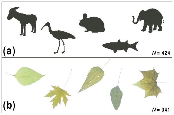
We collected shapes from two publicly available databases, one of animals (N = 424, drawn from the Brown LEMS lab animal database, collection #2; see http://www.lems.brown.edu/~dmc and Kimia, 2003), and the other of leaves (N = 341, drawn from the Smithsonian Leaves database; see Agarwal et al., 2006). Sample shapes from both sets are shown in Fig. 2. The shapes are simple silhouettes segregated from their original backgrounds. Obviously, there is no guarantee that these collections are statistically representative of their natural counterparts in every way. The shapes are often in canonical poses, and have been selected for use in these databases for a variety of reasons not related to the goals of our study. But nevertheless they serve as reasonable proxies of nature for the purposes of our inquiry, and provide a quantitative, empirical basis for the type of categorical distinctions that we wished to investigate.

Figure 2.

Sample shapes from the databases surveyed: (a) animals and (b) leaves. (Stimuli used in experiments were silhouettes drawn from images like those illustrated.)

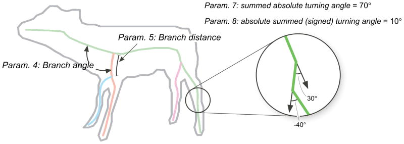
For each shape in the database, we computed shape skeletons using the methods presented in Feldman and Singh (2006), and then extracted several parameters from each skeleton. Our goal was to choose a set of skeletal parameters that were (a) relatively few in number (b) jointly sufficient to specify a skeleton and (c) approximately independent from each other. The chosen parameters included (1) total number of skeletal branches (parts); (2) maximum depth of the skeleton (depth is the degree of each branch in the hierarchy, with the root depth = 0, its children = 1, grandchildren = 2, etc.); (3) mean skeletal depth; (4) mean branch angle, i.e. the angle at which each (non-root) axis branches from its parent (see Fig. 3); (5) mean distance along each parent axis at which each child axis stems (see Fig. 3); (6) mean length of each axis relative to the root; (7) total absolute (unsigned) turning angle of each axis, i.e. the summed absolute value of the turning angle integrated along the curve (see Fig. 3); and (8) total (absolute value of) signed turning angle of each axis, integrated along the curve (see Fig. 3). Summed turning angles (both signed and unsigned) provide scale-invariant measures of contour curvature or “wiggliness” (see Feldman & Singh, 2005 for discussion). Note that (as can be seen in the example in the figure) they generally give different values, as Parameter 7 treats wiggles in opposite directions as cumulating, while Parameter 8 treats them as trading off. Again, these eight parameters are not the only choice possible (see Op de Beeck, Wagemans, & Vogels, 2001); they constitute a relatively simple set that approximately captures the structure of each shape’s parts and the relations among them. We also extracted several conventional non-skeletal parameters, including aspect ratio, compactness (perimeter²/area), symmetry, and contour complexity, to serve as comparisons.

Figure 3.

Illustration of several of the skeletal parameters used, branching angle and branching distance. In this figure, the number of branches is 4, the maximum depth is 2, and the average depth is 1.

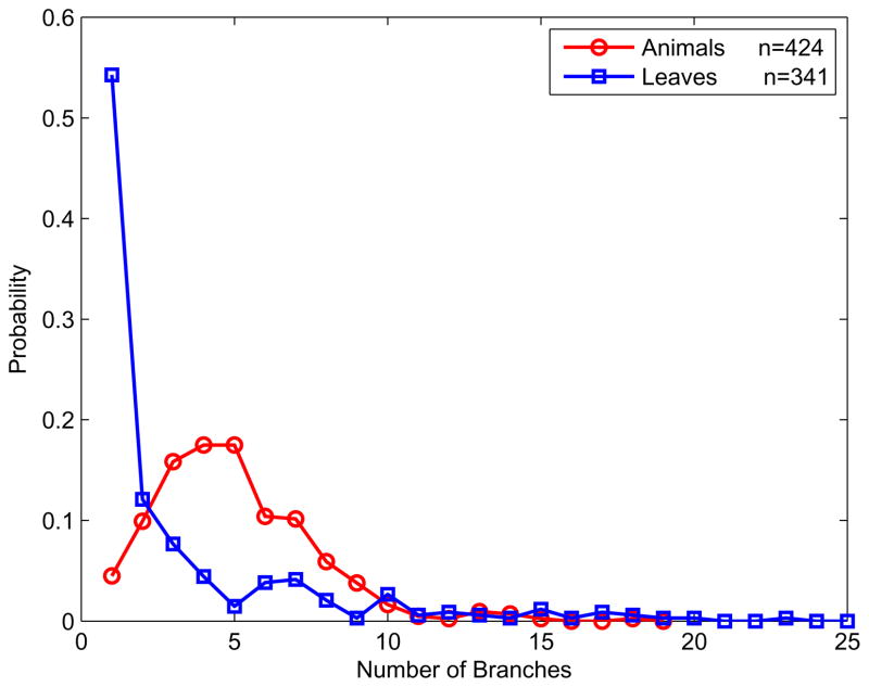
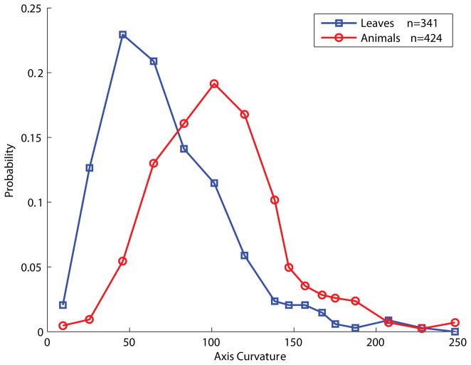
Among all the parameters sampled, several showed statistically meaningful differentiation between animal and leaf distributions, including the number of axes (Fig. 4) and the total signed turning angle (curvature) (Fig. 5). We used these distributions and several others to construct a simple Bayes classifier, which we present later in the paper when we compare its predictions to the results of the experiments.

Figure 4.

Distributions of the number of skeletal axes, showing animals (red) and leaves (blue).

Figure 5.

Distributions of the mean (signed) axial turning angle (curvature), showing animals (red) and leaves (blue).

The statistical distinctions between animals and leaves along these two parameters are highly suggestive of the respective shape-generating processes. For example, the number of axes in the animal shapes is approximately Gaussian (mean μ = 4.98, standard deviation σ = 2.58, fit to a Gaussian model R² = .90)² That is, as a category, animals tend to have about five parts, with variability on both sides of this mean. For quadrupeds, this count presumably correspond to about four legs plus the head, though it should be borne in mind that many of the animals in the database (as in nature) are not quadrupeds (including birds and hominids), some have not all limbs visible, some have tails, and so forth. But this very intuitive central tendency essentially reflects the accuracy of the MAP skeleton in estimating the true number of parts. By contrast, leaves have both lower mean number of parts (mean = 3.48), as well as a different distributional form: approximately exponential (rate parameter λ = 3.48, fit to an exponential model, R² = .97) with a long right-hand tail. Many leaves have only one part, while others have as many as 25, whereas no animal has more than 20. The exponential distribution suggests a recursive (self-similar or scale-invariant) branching process, similar to that of a river (Ball, 2001)—in contrast to the more stereotyped body plan common to most animals.

Similarly, the distributions of total axial turning angle (curvature) are approximately Gaussian for both animals and leaves (animals: μ = 108.3°, σ = 39.7°, fit to a Gaussian model R² = .98; leaves: μ = 74.1°, σ = 39.7°, fit to a Gaussian model R² = .90), with animals having more axis curvature (t(761) = 11.83, p < 2×10⁻¹⁶, Fig. 5). This difference presumably reflects the prevalence of articulated internal joints in animal (but not leaf) body plans.

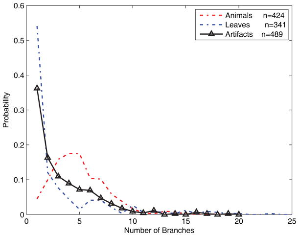
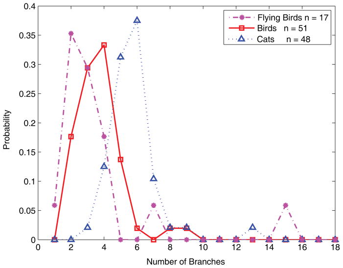
The current experiments involve only the distinction between animals and leaves, but other categories can be differentiated in a similar way. As illustration, Fig. 6 shows the distribution of one shape parameter (number of branches) for a collection of artifacts (drawn from the Princeton Shape Benchmark, see Shilane, Min, Kazhdan, & Funkhouser, 2004) with the animal and leaf distributions shown for comparison. As can be seen in the figure, the artifacts are readily distinguished from both animals and leaves, meaning that the likelihood ratio (ratio of the curves) is strongly biased through most of the range of the parameter. Simple skeletal shape parameters can also be used to distinguish subcategories, that is, categories at a lower level of the category hierarchy. Fig. 7 shows distributions for birds, cats, and one even more subordinate category, flying birds. As can be seen in the figure, all three categories are statistically distinguishable, and as one might expect the bird distribution falls in between flying birds and cats. Again, the details of these distributions are admittedly dependent on the peculiarities of the databases used; we give them only as a suggestive illustration of the broader applicability of the method.

Figure 6.

Distributions of the number of MAP skeletal branches for a set of artifacts (black). Animals (red) and leaves (blue) are redrawn from Fig. 4 for comparison.

Figure 7.

Distributions of the number of MAP skeletal branches, showing flying birds (magenta), profiles of birds (red), and cats (blue). Distinct distributions can be seen for different subsets of the animal class, suggesting that the methods described in this paper could be applied to more subordinate levels of the category hierarchy.

Experiments

Having established ecologically-informed statistical models of the shape skeletons in our two natural classes, we next asked how human subjects would assign shapes to the same two classes. In designing our experiments we wished to prevent our subjects from relying on overt recognition, in which they might (for example) classify a shape as an animal because they had first recognized it as an elephant. To accomplish this, we used artificial “blob” shapes that could not generally be definitively classified as any particular animal or leaf type, but which nevertheless exhibited variable degrees of “animalishness” or “leafishness.” We created shapes by morphing (linearly combining) animals and leaves from the same databases described above (details below), varying the proportion animal in order to create a wide variety of shapes with varying levels of apparent fit to the animal or leaf categories. Our goal was to induce subjects to gauge the more probable natural class without being able to identify a particular species, to reflect a subjective superordinate classification rather than overt recognition.

Experiment 1

In Exp. 1, we constructed novel shapes from linear combinations (“morphs”) of animal and leaf shapes with variable mixture weights, and asked subjects to classify them as animal or leaf using a key release. The dependent variables of interest was the probability of an animal response (= 1 - the probability of a leaf response), which we evaluated as a function of the mixture weight and of the skeletal parameters of the morphed composite shape.

Method

Subjects

Subjects were 28 undergraduates at Rutgers University participating in exchange for course credit. Subjects were naive to the purpose of the experiment.

Procedure and Stimuli

Stimuli were displayed on an iMac computer running Mac OS X 10.4 and Matlab 7.5, using the Psychophysics toolbox (Brainard, 1997; Pelli, 1997). The shapes were filled black regions on a white background, approximately 6 degrees of visual angle in size presented at approximately 61cm viewing distance.

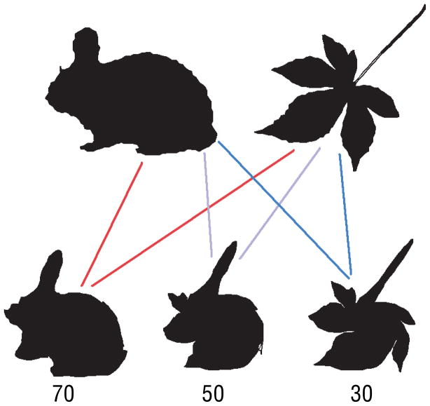
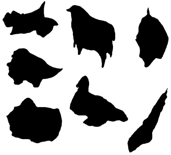
The shapes were constructed from weighted averages of animal and leaf shapes taken from the databases described above (250 shapes selected from each database). To make each morphed shape, two shapes were selected at random, one from the animal set and one from the leaf set. Each shape was sampled at 150 equally spaced points along the contour (sufficient to resolve all contour features discriminable in the original images). The two shapes were brought into approximate alignment by matching principal axes. Points in corresponding serial positions along the respective contours were then averaged, using a chosen weight (proportion animal = .3, .4, .5, .6, or .7) on the animal shape point and a complementary weight (proportion leaf, = 1 - proportion animal) on the leaf shape to yield a final morphed shape. Limiting the animal weight to a middle range of .3 – .7 means that the morphed shapes were never easily recognizable as specific categories of either animals or leaves, but rather retained substantial features of both classes (a fact reflected in the subjects’ responses reported below, which never reach the extremes of 0% or 100% that would have suggested overt recognition). For each subject, 250 shapes were constructed from novel random animal-leaf pairings, with equal numbers of trials using each of the five mixing proportions. This was done a second time in order to create a second block of trials. The two complete blocks were shown to subjects yielding a total of 500 trials. Fig. 8 illustrates the morphing procedure, and Fig. 9 shows examples of morphed shapes.

Figure 8.

Morphing procedure. Each stimulus shape was created by averaging the contour points from one animal shape and one leaf shape (top row), creating a set of novel shapes with various combination weights (bottom row). The numbers indicate proportion animal.

Figure 9.

Examples of morphed shapes used in the experiments.

Each subject was shown a random sequence of 500 shapes in random order, one shape per trial as described above, and were required to decide whether they thought a shape was “more likely” to be an animal or a leaf. Each trial began with a fixation mark. When ready, the subject pressed and held down the “A” key and the “L” key on the keyboard, one with each hand. The shape was displayed, and the subject indicated animal or leaf by lifting respectively either the “A” key or the “L” key. The stimulus shape remained on the screen until response. Following the trial the chosen key was displayed to confirm the intended response. No feedback was given, as there is no objectively correct response in this task. At the end of each trial fixation mark was displayed again to invite the subject to initiate the next trial.

Trials in which the subject responded with both keys were discarded, and a message displayed reminding the subject to choose only one response. Of the 14,000 total trials, 36 (0.25%) were removed.

Results and Discussion

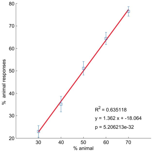
The subjects’ responses closely tracked the mixing weights used to create the morphed shapes shapes. Figure 10 shows the probability of an animal response as a function of the actual proportion animal. The response is strongly linear (R² = 0.64, p ≤ 5 × 10⁻³²), with a slope slightly larger than one and intercept slightly below zero (regression line y = 1.362x − 18%). This good fit was broadly consistent among subjects: individual fits (R² values) ranged from 0.67 to 0.99, with a mean of 0.93 and a standard deviation of 0.07. In other words, subjects were both consistent and effective at recovering the true source of the morphed shape, classifying it as an animal with a probability very close to the actual proportion animal used in creating it. Note that subjects’ mean response rates generally lie in the 20%–80% range, never reaching 0% or 100% animal, meaning that (as desired) subjects were generally unable to explicitly recognize specific types of animals or leaves, but instead responded in accordance with a more subjective evaluation of animal-like or leaf-like form.

Figure 10.

Exp. 1 results. The plot shows subjects’ classifications (mean percent animal response) as a function of mixture proportion (percent animal), averaged across trials and subjects. Error bars indicate ± one standard error.

Analyses of reaction times showed a significant correlation between the probability of an animal response and response latency (r = 0.7691, p = 0.00002). However, this high correlation seems to be due to reaction times greater than 10 seconds (about 0.57% of the trials). With these 80 trials (of the total 13964) removed, the correlation disappears (r = 0.2947, p > 0.2), suggesting that reaction time is not related to response category. An ANOVA confirmed that the distributions of reaction times were not significantly different across weights (F_4,115 = 1.30487 × 10⁻⁰⁶, p ≈ 1), suggesting a uniformly easy and automatic categorization process.

These results essentially provide a “sanity check,” confirming that subjects found the task comprehensible, readily classifying novel shapes into natural classes in a consistent manner consonant with the true origins of each shape. The more critical analysis involves understanding what factors actually influenced their classifications—that is, what properties of the novel shapes actually induced them to classify a given object one way or the other. (Obviously the mixing proportion is unknown to subjects, but rather is being effectively estimated on the basis of observable properties of the shape.) We defer this analysis until after presenting the results Exp. 2, when we introduce a classifier model and evaluate it with respect to the results of both experiments.

Experiment 2

As mentioned above, a sizeable body of studies has shown that subjects are able to classify natural scenes even after extremely rapid, masked presentation (Bacon-Macé, Macé, Fabre-Thorpe, & Thorpe, 2005; Fabre-Thorpe, Delorme, Marlot, & Thorpe, 2001; Thorpe et al., 1996; VanRullen & Thorpe, 2001). Several authors have argued that such classifications may be carried out by an initial stage of feedforward processing, potentially distinct from later, slower perceptual mechanisms that involve recurrent computation and selective attentive. This raised in our minds the possibility that we might obtain different results in our shape classification task under rapid, masked conditions. (Recall that in Exp. 1 shapes remained onscreen until response.) We conducted another study with an identical design except that shapes were presented briefly and followed by a mask.

Experiment 2

Method

Subjects

Twenty-one new subjects participated in the experiment in exchange for class credit. Subjects were naive to the purpose of the experiment.

Procedure and Stimuli

The stimulus shapes were identical to those used in Exp. 1. Each trial began with a fixation cross. As in Exp. 1, the subject initiated each trial by pressing the “A” and “L” keys. The stimulus display length was randomly selected from one of three exposure durations: short (50 ms), medium (100 ms), or long (200 ms). Following the disappearance of the stimulus there was a 12.5 ms blank screen, followed by a mask displayed for 100 ms. Masks were created from shape pieces cut out from the stimulus set. On each trial a mask was chosen randomly from a set of seven possibilities. Following the disappearance of the mask the subject would release one of the keys to respond. Their response then appeared on the screen and the next trial would start. Each experimental session included 500 trials, lasting about half an hour.

Results and Discussion

The three exposure durations (small, medium, and long) did not result in significantly different mean responses (F_2,219 = 1.89 and p = 0.15). Hence data from the three conditions were collapsed over for the remainder of the analysis.

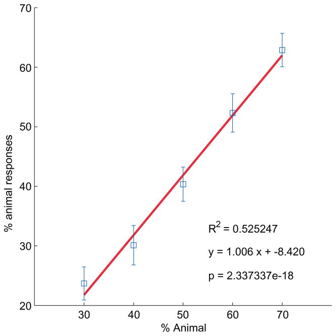
Results from Exp. 2 were broadly similar to those from Exp. 1, with several small but intriguing differences. Mean probability of an animal response again closely matched the actual mixing proportion (Figure 11), R² = 0.53, p < 2 × 10⁻¹⁸, y = 1.01x − 8.4%). However the regression line has a lower slope than in Exp. 1 (1.01 in Exp. 2 vs. 1.36 in Exp. 1, t = 2.74, p < 0.01), suggesting that subjects’ sensitivity to the animal likelihood was slightly altered by the limited viewing time (see Ons, De Baene, & Wagemans, in press). Subjects in Exp. 2 seem to have used a narrower range of responses, never reaching above about 65% animal responses, while mean responses rose to about 80% in Exp. 1. This might reflect a difference in criterion, with the limited presentation time in some way inducing a “leaf bias,”, perhaps by impeding subjects from reaching their internal threshold for responding animal.

Figure 11.

Exp. 2 results. The plot shows subjects’ classifications (mean percent animal response) as a function of mixture proportion (percent animal), averaged across trials and subjects. Error bars indicate ± one standard error.

Notwithstanding these relatively subtle differences in the pattern of data, the overall pattern of results was essentially the same as in Exp. 1; the brief exposure in Exp. 2 did not substantially alter the strategy or mechanisms employed by subjects. Largely regardless of the duration of exposure, subjects were able to achieve broad consensus as to probable class membership over an extremely wide variety of shapes. We next turn to the more fundamental question of how they accomplished this.

Modeling

Our main goal is to investigate whether subjects’ classification responses can be understood as the result of a statistical evaluation of the parameters of the observed shape and its shape skeleton. To this end, we constructed a family of simple Bayes classifiers using subsets of the eight skeleton parameters introduced above, applying likelihood models drawn from the shape databases (the original un-morphed shapes).

The first step is to exclude parameters that are not informative about the target distinction animal vs. leaf. We compared the animal and leaf distributions along each of the eight parameters, evaluating the difference between the two distributions. As several of the distributions did not appear to be normally distributed, we used the nonparametric Wilcoxon rank sum test (Mann-Whitney U). Three of the parameters (branch length, distance along parent at which a child branches, and the angle at which each child branches from its parent) failed to show a significant differences (using significance criterion α = .01) and were excluded from further analysis. The remaining five parameters showed significant differentiation of animal and leaf classes, and thus have at least the potential to enhance the performance of the classifier.

The next step is to construct a classifier over each parameter. For the i-th parameter (say, total turning angle), the animal and leaf classes respectively have distributions p(x_i|animal) and p(x_i|leaf), where x_i is the value of object x along the i-the parameter. To construct a Bayes classifier, we take these distributions as likelihood functions for the two classes, and estimate them from the database surveys presented above. We assume equal priors, p(animal) = p(leaf), which is true in the set of shapes from which our morphed shapes were constructed. Applying Bayes’ rule, the posterior probability that a given shape x_i belong to the animal class will then just be

$$p(\text{animal}\mid x_i)=\frac{p(x_i\mid \text{animal})}{p(x_i\mid \text{animal})+p(x_i\mid \text{leaf})},$$ (1)

where again x_i denotes the value of shape x along the i-th parameter. The value of this posterior depends on the likelihood ratio between the animal and leaf classes,

$$L_i=\frac{p(x_i\mid \text{animal})}{p(x_i\mid \text{leaf})},$$ (2)

which expresses how strongly the evidence (the shape’s value along parameter x_i) speaks in favor of an animal classification relative to a leaf one. To combine information from the k parameters, we make the simple assumption that they are independent. (This assumption makes this a “naive” classifier; in Bayesian theory, the term “naive” refers to an assumption of independence among parameters whose dependencies are unknown; e.g. see Duda, Hart, & Stork, 2001.) This assumption means that the likelihoods multiply:

$$L=\prod _{i=1}^k\frac{p(x_i\mid \text{animal})}{p(x_i\mid \text{leaf})}$$ (3)

or if we take logs, add:

$$logL=\sum _{i=1}^{k}logp(x_i\mid \text{animal})-\sum _{i=1}^{k}logp(x_i\mid \text{leaf}).$$ (4)

This leads to a simple linear classifier rule: respond animal if the log likelihood exceeds some criterion c,

$$logL>c.$$ (5)

The criterion c could be set to zero, or some other value if we relax the assumption of equal priors. The normative criterion is

$$c=logp(\text{leaf})-logp(\text{animal}),$$ (6)

which is zero if and only if the priors are equal. This classifier corresponds to a decision rule by which the observer collects k parameters from the shape, evaluates each one with respect to how strongly it implies animal or leaf, aggregates evidence from all the parameters linearly, and responds animal if the sum exceeds criterion and leaf otherwise.

To further tune the classifier, we ran it using all possible subsets of the five informative parameters, a total of 31 (= 2⁵ − 1) combinations. We used the AIC (Akaike, 1974) to appropriately penalize overfitting due to variations in the number of parameters, attempting to find a combination with both a good fit to the training data as well as a small number of parameters. The model with overall minimum (winning) AIC used two parameters: (1) the number of skeletal branches, and (2) the total signed axial turning angle (curvature). This model classifies about 81% of the training data correctly. Using leave-one-out cross validation the model still performs at 79.6% correct. (But note that the real test of the model is in the comparison to human performance on the morphed shapes, below.) Eight models (including this one) all had similar AIC values, each of which included some combination of the number of branches, the signed axis turning angle, and the unsigned axis turning angle, corroborating the utility of these parameters. Another parameter, the average depth of a skeletal branch, also appeared is several of the top eight models, but not in the top two, and did not improve the classifier’s performance. So as our final model we chose the two-parameter model (branch number and signed axis turning angle, distributions of which are plotted in Fig. 4 and 5), which had minimum AIC. We repeated these comparisons using the BIC (Schwarz, 1978) and found the same eight closely clustered models, giving a desirable corroboration that the final 2-parameter model simultaneously maximizes effectiveness and simplicity.

Although the model based on the two skeletal parameters performed well on the training shapes, its performance is far from perfect, and one might wonder how well human subjects would perform on these “unadulterated” shapes. (Recall that in the experiments subjects only saw morphed shapes, not the original ones.) In order to address this question, we separately ran a new group of 8 subjects on a version of Exp. 2 in which only the original animal and leaf shapes were shown, i.e., with mixing proportions of 0 and 100% (with a presentation time of 50msec). Subjects’ mean accuracy on these shapes was 88.8% (s.d 3%), with no subject performing better than 95%—as compared to about 80% correct classification by the model. In other words, we found that human subjects are also far from perfect on the training shapes. In comparing these results to those of Thorpe et al. (1996) and VanRullen and Thorpe (2001), one should bear in mind that our stimuli are by design much more impoverished than those used in those studies, which makes the subjects’ task considerably more difficult.

Fit of the Bayesian classifier to human data

We next applied the naive skeletal classifier to the novel morphed shapes used in the experiments, comparing its responses to those of the subjects. (Recall that the classifier was trained on the original label shapes from the databases, not the morphed shapes that the subjects saw, so this evaluation is completely independent from the training.) We also constructed several alternative models using more conventional non-skeletal shape parameters for comparisons.

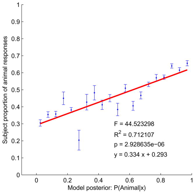
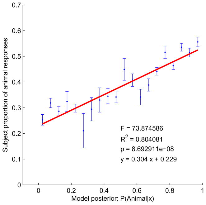
For the naive skeletal classifier, fit to the human data was very good (Exp. 1: Fig. 12; Exp. 2: Fig. 13). Both plots show a strong linear relationship between the posterior, p(animal|x) (Eq. 1), and the observed proportion animal responses (Exp. 1: y = .334x + 0.293, R² = .71, p < 2.93 × 10⁻⁶; Exp. 2: y = 0.304x + 0.229, R² = 0.80, p < 8.7 × 10⁻⁸). The close fit means that human subjective judgments of “animalishness” correspond closely to the Bayesian estimate of the probability of the animal class. In this sense humans can be thought of as approximately rational animal/leaf classifiers, given an ecologically tuned model of the statistical differences between the shapes in the two categories. Again, we see little difference between the free-viewing (Exp. 1) and masked (Exp. 2) conditions, suggesting that the relevant representations are formed quickly and not revisited.

Figure 12.

Fit of the Bayesian skeletal classifier to human responses, Exp. 1. The plot shows proportion animal responses as a function of the animal posterior. Error bars represent ± 1 standard error. Shapes with similar posteriors have been binned so that the proportion of animal responses could be calculated.

Figure 13.

Fit of the Bayesian skeletal classifier to human responses, Exp. 2. The plot shows proportion animal responses as a function of the animal posterior. Shapes with similar posteriors have been binned so that the proportion of animal responses could be calculated. Bins with only a single shape have undefined standard error so no error bar is shown.

It should be emphasized that the main conclusion of this near-optimal behavior, especially given the very small number of parameters used, is that the parameters on which we have based the classifier—a few simple properties of the shape skeleton—were well chosen. With a sufficiently rich representation, it would be no surprise that subjects can effectively compute similarities to animals and leaves they have seen before. What is more impressive is that they seem to use only a few parameters to do so, implying that the shape-generating models we have identified correspond closely to their underlying representation.

Alternative models

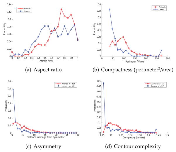
We wished to confirm that the good performance of our classifier could not be matched using more conventional non-skeletal shape properties, and so we constructed alternative classifiers from several other well-known shape parameters. One natural candidate is aspect ratio (the ratio of the shape’s longest dimension to its perpendicular shorter dimension), which is a basic property of global shape and has been shown to be psychologically meaningful (Feldman & Richards, 1998). Another common and easily computed shape parameter is compactness (perimeter²/area), which deWinter and Wagemans (2008) have shown is related to subjective part salience. Another well-known global shape property is (a)symmetry, which we compute by calculating the Hausdorff distance between one half of the shape and the other half, minimizing over all possible reflection axes. Finally, we also use a measure of contour complexity proposed in Feldman and Singh (2005), which measures the degree of unpredictable undulation along the length of a contour. The contour complexity is the integrated surprisal or description length along the contour, i.e. the sum -Σ_i ln p(α_i) (where the α_i are the sequence of turning angles along the sampled contour) and is expressed in base-e bits or nats. For each of these parameters, just as with our skeletal parameters, we evaluated each shape in the two shape databases and tabulated statistics. Fig. 14 shows two class-conditional distributions for the four parameters. All four parameters show significant differences between animal and leaf classes by nonparametric tests (Wilcoxon rank-sum test: different at p ≤ 4.6 × 10⁻⁷ for aspect ratio, p ≤ 6.5 × 10⁻²⁴ for compactness, p < 1.3x10⁻⁴³ for symmetry, and p < 1.1x10⁻³² for contour complexity), confirming that they are at least potentially useful in discriminating animals from leaves. Fig. 14 shows the animal and leaf distributions for each parameter.

Figure 14.

Animal vs. leaf distributions for (a) aspect ratio (b) compactness (perimeter²/area), (c) asymmetry (d) contour complexity. Each of these parameters is potentially useful for distinguishing animals vs. leaves, in that the distributions are markedly different (decisive likelihood ratio in most of the range). But in each case the data show that classifiers built from these parameters do not explain the data as well as our proposed model.

Next, we constructed classification models over these parameters, meaning for each one a classifier that computes the animal posterior p(animal|x) for each respective parameter x. On the training set the models based on aspect ratio, compactness, symmetry, and contour complexity classify at 72%, 83%, 82%, and 79% respectively.

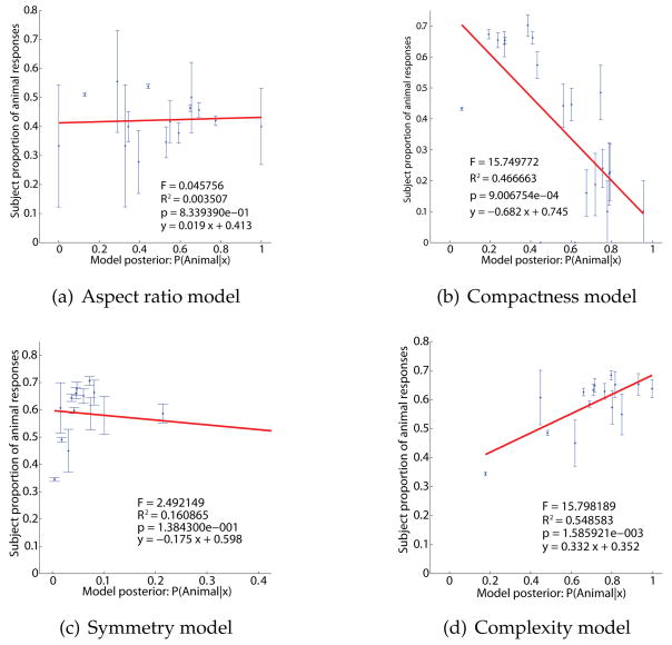
The main question is how each of these models predicts human classification of the morphed shapes. Fig. 15 show the resulting fits (mean probability of an animal response as a function of the model animal posterior, Exp. 1 data). In each case the fit is either poor or negative. The fit for the aspect ratio and symmetry models are nonsignificant (aspect ratio: R² < .009, p > .5; symmetry: R² = .16, p > .1), showing no statistically meaningful relationship between predicted and observed responses. For compactness, the fit is significant (R² = .47, p = .001) but the regression runs in the wrong direction, with animal responses primarily decreasing as animal posterior increases. Only contour complexity is a significant predictor of human responses (R² = .55, p < .005), though the R² is substantially smaller than that of the skeletal classifier. Hence even though aspect ratio, compactness, and symmetry are each potentially informative in discriminating animals from leaves, our subjects apparently did not use them; evidence from these parameters that should have (say) increased the probability of the animal class was not generally interpreted as doing so by subjects. In the case of compactness, the available evidence was systematically misinterpreted: shapes whose properties more closely matched those of animals were actually more likely to be classified as leaves.

Figure 15.

Fit of several alternative models to human data. Each model is a classifier along a different shape parameter, respectively (a) aspect ratio (b) compactness (perimeter²/area) (c) asymmetry and (d) contour complexity. In each case the plot shows proportion animal responses as a function of the given model’s animal posterior. For aspect ratio (a) and symmetry (c) there is no relationship, meaning that subjects’ responses are not related to these parameters. For compactness the relationship is negative, meaning that as animal posterior rises, subjects’ animal responses actually decrease. Only for contour complexity (d) do human animal responses rise with the classifier’s animal posterior, meaning that more complex shapes were generally more likely to be classified as animals; but the relationship (R² = .55) is substantially weaker than for our skeletal model (R² = .71), Fig. 12.

These results strongly corroborate our conclusion that subjects’ responses can be understood as reflecting a posterior computed with respect to a few skeletal parameters, but do not reflect other salient shape properties, even when those properties are objectively useful in discriminating animals from leaves. Subjects’ shape classifications can be understood as a simple statistical decision reflecting skeletal properties in particular.

General discussion

The main conclusion of this study is that subjects’ classifications of shapes into our two natural categories can be well modeled by a Bayesian classifier using a very small number of shape skeleton parameters, in which the model’s assumptions (i.e., its likelihood model) are consistent with the empirical distribution in naturally-occurring shapes. In effect the classifier applies a “stereotype” of animals as shapes with multiple relatively curvy limbs, and leaves as shapes with fewer, straighter, limbs. Subjects share this stereotype and apply it in a similar way, as evidenced by the very close fit between the subjects’ responses and those of the Bayes classifier. It should be kept in mind that the shapes in the experiments cannot be definitively recognized as any particular real species or category, because they are all artificial morphs with characteristics of both classes. So neither the subjects nor the classifier should be thought of as recognizing shapes, but rather classifying novel shapes as animal-like or leaf-like. The data suggests that subjects carry out this subjective evaluation by means of a simple statistical classification of the shape skeleton.

These results add to the literature establishing the psychological reality of shape skeletons and medial axis representations (Burbeck & Pizer, 1995; Harrison & Feldman, 2009; Kimia, 2003; Kovacs & Julesz, 1994; Kovacs et al., 1998; Psotka, 1978), showing how skeletal structure relates to superordinate shape categories. Most shape representation schemes are based on the bounding contour and do involve any overt representation of global shape or medial axes. But many authors (e.g. Sebastian & Kimia, 2005; Siddiqi, Tresness, & Kimia, 1996) have argued that shape cannot be understood entirely in terms of local contour structure, and that global aspects of form must be involved. Our results demonstrate clearly that global form in general, and shape skeletons in particular, are potentially informative about natural shape categories and moreover are actually used by human subjects when classifying shapes.

We found no pronounced difference in performance between free-viewing conditions (Exp. 1) and rapid, masked presentation (Exp. 2). We cannot draw any strong conclusion from the absence of a difference, but it tends to suggest that the human responses in this task proceed based on a very rapid (feed-forward) computation of the shape skeleton that is substantially unaffected by the availability of more processing time. This is consistent with the suggestion by Lee, Mumford, Romero, and Lamme (1998) that medial representations might be computed as early as V1, and more broadly with the argument by Kimia (2003) that they are central to many areas of visual form analysis. The development of more rapid computational methods for computing shape skeletons thus remains a key goal both for computational applications (Sebastian & Kimia, 2005) and for modeling of human form processing.

Conclusion

Most broadly, our results argue for a “naturalization” of shape representations. This is a far-reaching program that has fundamental implications for shape representation, in that it places potentially heavy constraints on the shape parameters to be extracted. Historically, most approaches to shape representation have been based only on abstract geometric considerations, with little attention to the probabilistic tendencies of natural shapes. Of course, several important approaches have taken natural shape regularities as a basic motivation. A prominent example is the minima rule of Hoffman and Richards (1984), who argued that deep concavities (extrema of negative curvature) tend to arise whenever approximately convex parts interpenetrate. They described this principle (transversality of parts; Bennett & Hoffman, 1987) as a regularity of nature—a mathematical consequence of some very general assumptions about the structure of natural forms, such as that parts tend to be convex while part orientations tend to be independent (and thus generically transverse). Similarly Feldman and Singh (2005) have argued that positive contour curvature in principle has higher probability than negative curvature—again, a basic mathematical constraint stemming from geometry. The relative frequency of cortical cells tuned to positive vs. negative contour curvature has been attributed to differences in the frequency with which each type of curvature is encountered in the environment (Pasupathy & Connor, 2002). But the empirical distribution of curvature in real shapes has only begun to be explored (Ren, Fowlkes, & Malik, 2008), and empirical distributions of most other shape properties have not been explored at all.

Our results go further in showing that individual shape parameters can be evaluated in a way that reflects specific quantitative knowledge of natural shape statistics, and that if this knowledge is correctly “tuned” the resulting classifications can produce semantically useful categorical distinctions. Naturally, we do not expect that knowledge of the statistics of shape would extend into the fine details of the distributions, which vary from environment to environment (e.g. leaves are narrower in northern latitudes; snakes are absent from Ireland, increasing the mean number of parts in the animal class; etc.) Rather, the knowledge that might be reasonably encoded in fundamental mental shape parameters would be of a more general kind, such as the existence of broad natural classes such as animals, leaves, rocks, trees, and other humans, along with knowledge of the parameters that might be informative in distinguishing these classes. In this sense our results suggest that human shape representation gives a central role to skeletal parameters—encoding the part hierarchy, the approximate shapes of parts and their axes, and the spatial relations among them. Extraction of these parameters is best understood in the context of a broader picture of superordinate classification as providing an interface between rapidly evaluated perceptual properties and more meaningful inferences with important implications for behavior (Richards & Bobick, 1988; Torralba & Oliva, 2003).

Appendix: Synopsis of Bayesian estimation of the shape skeleton

Here we give a brief synopsis of Bayesian skeleton estimation, which was introduced in Feldman and Singh (2006). As explained in the text, the goal of this approach is to use an inverse-probability framework to estimate the skeleton most likely to have generated the observed shape SHAPE, which is assumed to comprise a set of N contour points x₁ … x_N with associated normal vectors n_i … n_N. We assume each shape was generated by a skeleton SKEL, which is a hierarchically organized ensemble of K axes, including a root axis, children, grandchildren, etc. (Distinct axes are illustrated with distinct colors in the figures; the specific colors are arbitrary.) The likelihood model specifies exactly how shapes are generated from skeletons, and with what probabilities, while the prior defines the probability of any given skeleton purely on the basis of its structure, independent of its fit to any particular shape. The assumptions about the prior and likelihood given here are generic, in that they are not particularized to specific shape classes, but note that one goal of the current paper is to understand how probabilistic models of distinct shape classes in fact differ, which would be reflected in class-specific modifications of these assumptions.

To construct a prior over skeletons p(SKEL), we assume that turning angles α from point to point within each axis are generated from a von Mises distribution α ∝ exp (B cos α) (approximately equivalent to a Gaussian, but appropriate for angles). This means that at each point the axis is most likely to continue straight, but may deviate to the right or left with probability that diminishes with increasingly large deviations, an assumption that is supported by a variety of mathematical arguments and a great deal of empirical data (Feldman & Singh, 2005). Each axis itself has prior probability p_A. The axes are assumed to be independent from each other, and likewise the turning angles along each axis, so all these priors multiply to yield

$$p(\text{SKEL})=\prod _i^K{p}_{A}p({\alpha }_j)=p_a^K\prod _{j}p({\alpha }_j),$$

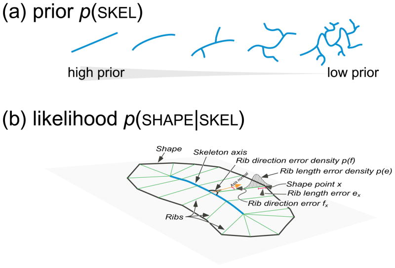
where the product of the p(α_j) runs along all the axes. This expression assigns high priors to skeletons with few axes, and to those with relatively straight axes (Fig. 16a)—that is, it favors simple skeletons.

Figure 16.

Schematic illustration of (a) the prior over skeletons p(SKEL), and (b) the likelihood model p(SHAPE|SKEL).

$$-logp(\text{SKEL}\mid \text{SHAPE})\propto -logp(\text{SHAPE}\mid \text{SKEL})+-logp(\text{SKEL})\propto \text{DL}(\text{SHAPE}\mid \text{SKEL})+\text{DL}(\text{SKEL}).$$

For the likelihood function, we assume that axis points generate random vectors laterally (on both sides of the axis) in random directions and at random distances. The random vectors, referred to as ribs, represent correspondences between axis points and contours points, determining which axis point is interpreted as “explaining” (being the generative source of) which contour points. (The ribs are shown in Fig. 17 with colors matching the axis to which they belong.) Ribs are assumed to be generated from the axis in a direction that has mean perpendicular to the axis (on both sides) with a von Mises directional error f_x, and to have length chosen from a mean determined within a window along the axis (to enforce smoothness) plus a Gaussian error e_x.

Figure 17.

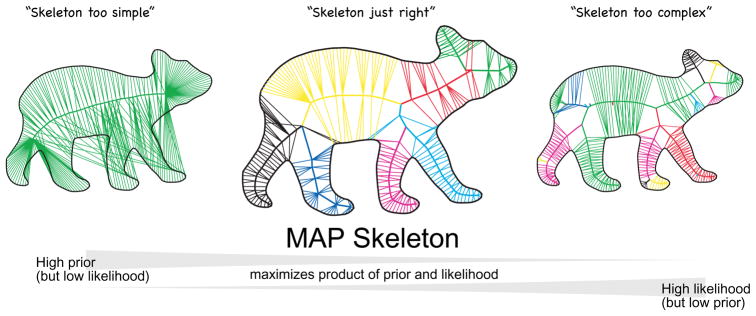
Simple skeleton have high prior (left), but fit the shape poorly (low likelihood); complex skeletons (right) have lower prior but fit the shape better (high likelihood). The MAP skeleton (center) maximizes the product of prior and likelihood, and is “just right.”

Finally a skeleton is chosen—the MAP skeleton—that maximizes the posterior (i.e. maximizes the product of the prior and likelihood, which is the numerator of the posterior). Because of the simplicity-based prior, the posterior maximization inherently optimizes the balance between skeletal simplicity and fit to the shape, identifying a skeleton that is neither too simple to fit the shape well, nor too complex to have a high prior (overfitting the shape), but rather represents an optimal combination of fit and complexity (Fig. 17). In this sense, given the assumptions made in the prior and in the likelihood, the MAP skeleton is the optimal interpretation of the shape. This is essentially why its axes correspond to intuitive parts, because only those axes whose benefit in descriptive power outweighs the complexity they add are components of the winning skeleton. Moreover the MAP skeleton can also be regarded as the simplest interpretation of the shape, in the sense that it minimizes the Shannon description length (Rissanen, 1978; see Chater, 1996). To find the skeleton that maximizes the posterior (and minimizes description length), we use the approximate techniques described in Feldman and Singh (2006).

References

- Agarwal G, Belhumeur P, Feiner S, Jacobs D, Kress JW, Ramamoorthi RNB, et al. First steps toward an electronic field guide for plants. Taxon. 2006;55:597–610. [Google Scholar]
- Akaike H. A new look at the statistical model identification. IEEE Transactions on Automatic Control. 1974;19(6):716–723. [Google Scholar]
- Annis, Frost Human visual ecology and orienation anisotropies in acuity. Science. 1973;182(4113):729–731. doi: 10.1126/science.182.4113.729. [DOI] [PubMed] [Google Scholar]
- Bacon-Macé N, Macé MJM, Fabre-Thorpe M, Thorpe SJ. The time course of visual processing: backward masking and natural scene categorisation. Vision Research. 2005;45:1459–1469. doi: 10.1016/j.visres.2005.01.004. [DOI] [PubMed] [Google Scholar]
- Baddeley R. The correlational structure of natural images and the calibration of spatial relations. Cognitive Science. 1997;21(3):351–372. [Google Scholar]
- Ball P. The self-made tapestry: pattern formation in nature. Oxford: Oxford University Press; 2001. [Google Scholar]
- Barenholtz E, Feldman J. Visual comparisons within and between object parts: evidence for a single-part superiority effect. Vision Research. 2003;43(15):1655–1666. doi: 10.1016/s0042-6989(03)00166-4. [DOI] [PubMed] [Google Scholar]
- Bennett B, Hoffman D. Shape decompositions for visual recognition: The role of transversality. In: Richards WA, editor. Image understanding. New Jersey: Ablex; 1987. pp. 215–256. [Google Scholar]
- Biederman I. Recognition-by-components: A theory of human image understanding. Psychological Review. 1987;94(2):115–147. doi: 10.1037/0033-295X.94.2.115. [DOI] [PubMed] [Google Scholar]
- Blum H. Biological shape and visual science (part 1) Journal of Theoretical Biology. 1973;38:205–287. doi: 10.1016/0022-5193(73)90175-6. [DOI] [PubMed] [Google Scholar]
- Blum H, Nagel RN. Shape description using weighted symmetric axis features. Pattern Recognition. 1978;10:167–180. [Google Scholar]
- Brady M, Asada H. Smoothed local symmetries and their implementation. International Journal of Robotics Research. 1984;3(3):36–61. [Google Scholar]
- Brainard D. The psychophysics toolbox. Spatial Vision. 1997;10:433–436. [PubMed] [Google Scholar]
- Brunswik E. Perception and the representative design of psychological experiments. Berkely, CA: University of California Press; 1956. [Google Scholar]
- Brunswik E, Kamiya Ecological cue-validity of ’proximity’ and of other gestalt factors. The American Journal of Psychology. 1953;66(1):20–32. [PubMed] [Google Scholar]
- Burbeck C, Pizer S. Object representation by cores: identifying and representing primitive spatial regions. Vision research. 1995;35:1917–1930. doi: 10.1016/0042-6989(94)00286-u. [DOI] [PubMed] [Google Scholar]
- Chater N. Reconciling simplicity and likelihood principles in perceptual organization. Psychological Review. 1996;103(3):566–581. doi: 10.1037/0033-295X.103.3.566. [DOI] [PubMed] [Google Scholar]
- Chellappa R, Bagdazian R. Fourier coding of image boundaries. IEEE Transactions on Pattern Analanysis and Machine Intelligence. 1984;6(1):102–105. doi: 10.1109/tpami.1984.4767482. [DOI] [PubMed] [Google Scholar]
- de Winter J, Wagemans J. Segmentation of object outlines into parts: A large-scale integrative study. Cognition. 2006;99(3):275–325. doi: 10.1016/j.cognition.2005.03.004. [DOI] [PubMed] [Google Scholar]
- de Winter J, Wagemans J. Perceptual saliency of points along the contour of everyday objects: A large-scale study. Perception & Psychophysics. 2008;70(1):50–64. doi: 10.3758/pp.70.1.50. [DOI] [PubMed] [Google Scholar]
- Duda RO, Hart PE, Stork DG. Pattern classification. New York: John Wiley and Sons, Inc; 2001. [Google Scholar]
- Fabre-Thorpe M, Delorme A, Marlot C, Thorpe S. A limit to the speed of processing in ultra-rapid visual categorization of novel natural scenes. Journal of Cognitive Neuroscience. 2001;13(2):171–180. doi: 10.1162/089892901564234. [DOI] [PubMed] [Google Scholar]
- Feldman J, Richards WA. Mapping the mental space of rectangles. Perception. 1998;27:1191–1202. doi: 10.1068/p271191. [DOI] [PubMed] [Google Scholar]
- Feldman J, Singh M. Information along contours and object boundaries. Psychological Review. 2005;112(1):243–252. doi: 10.1037/0033-295X.112.1.243. [DOI] [PubMed] [Google Scholar]
- Feldman J, Singh M. Bayesian estimation of the shape skeleton. Proceedings of the National Academy of Sciences. 2006;103(47):18014–18019. doi: 10.1073/pnas.0608811103. [DOI] [PMC free article] [PubMed] [Google Scholar]
- Field D. Relations between the statistics of natural images and the response properties of cortical cells. Journal of the Optical Society of America. 1987;4:2379–2394. doi: 10.1364/josaa.4.002379. [DOI] [PubMed] [Google Scholar]
- Freeman H. On the encoding of arbitrary geometric configurations. IRE Transactions on Electronic Computers. 1961;EC-10:260–268. [Google Scholar]
- Fu KS. Syntactic methods in pattern recognition. New York, NY: Academic Press; 1974. [Google Scholar]
- Geisler WS. Visual perception and the statistical properties of natural scenes. Annual Review of Psychology. 2008;59:167–192. doi: 10.1146/annurev.psych.58.110405.085632. [DOI] [PubMed] [Google Scholar]
- Geisler WS, Diehl RL. Bayesian natural selection and the evolution of perceptual systems. Phil Trans R Soc Lond B. 2002;(357):419–448. doi: 10.1098/rstb.2001.1055. [DOI] [PMC free article] [PubMed] [Google Scholar]
- Geisler WS, Diehl RL. A bayesian approach to the evolution of perceptual and cognitive systems. Cognitive Science. 2003;27:379–402. [Google Scholar]
- Geisler WS, Perry JS, Super BJ, Gallogly DP. Edge co-occurrence in natural images predicts contour grouping performance. Vision Research. 2001;41:711–724. doi: 10.1016/s0042-6989(00)00277-7. [DOI] [PubMed] [Google Scholar]
- Gibson J. The senses considered as perceptual systems. Houghton: Mifflin; 1966. [Google Scholar]
- Gonzalez R, Woods R. Digital image processing. Reading, MA: Addison-Wesley; 1992. [Google Scholar]
- Goshtasby A. Description and discrimination of planar shapes using shape matrices. IEEE Transactions on Pattern Analysis and Machine Intelligence. 1985;7:738–743. doi: 10.1109/tpami.1985.4767734. [DOI] [PubMed] [Google Scholar]
- Harrison SJ, Feldman J. Influence of shape and medial axis structure on texture perception. Journal of Vision. 2009;9(6):1–21. doi: 10.1167/9.6.13. [DOI] [PubMed] [Google Scholar]
- Hirsch HB, Spinelli DN. Visual experience modifies distribution of horizontally and vertically oriented receptive fields in cats. Science. 1970;168(3933):869–871. doi: 10.1126/science.168.3933.869. [DOI] [PubMed] [Google Scholar]
- Hoffman DD, Richards WA. Parts of recognition. Cognition. 1984;18(1–3):65–96. doi: 10.1016/0010-0277(84)90022-2. [DOI] [PubMed] [Google Scholar]
- Hoffman DD, Singh M. Salience of visual parts. Cognition. 1997;63:29–78. doi: 10.1016/s0010-0277(96)00791-3. [DOI] [PubMed] [Google Scholar]
- Hubel DH, Wiesel TN. The period of susceptibility to the physiological effects of unilateral eye closure in kittens. J Physiol. 1970;206:419–436. doi: 10.1113/jphysiol.1970.sp009022. [DOI] [PMC free article] [PubMed] [Google Scholar]
- Katz RA, Pizer SM. Untangling the Blum medial axis transform. International Journal of Computer Vision. 2003;55(2/3):139–153. [Google Scholar]
- Kimia BB. One the role of medial geometry in human vision. Journal of Physiology Paris. 2003;97:155–190. doi: 10.1016/j.jphysparis.2003.09.003. [DOI] [PubMed] [Google Scholar]
- Kovacs I, Feher A, Julesz B. Medial-point description of shape, a representation for action coding and its psychophysical correlates. Vision Research. 1998;38:2323–2333. doi: 10.1016/s0042-6989(97)00321-0. [DOI] [PubMed] [Google Scholar]
- Kovacs I, Julesz B. Perceptual sensitivity maps within globally defined visual shapes. Nature. 1994;370:644–646. doi: 10.1038/370644a0. [DOI] [PubMed] [Google Scholar]
- Lee TS, Mumford D, Romero R, Lamme VAF. The role of the primary visual cortex in higher level vision. Vision Research. 1998;38:2429–2454. doi: 10.1016/s0042-6989(97)00464-1. [DOI] [PubMed] [Google Scholar]
- Leyton M. A process-grammar for shape. Artificial Intelligence. 1988;34:213–247. [Google Scholar]
- Leyton M. Inferring causal history from shape. Cognitive Science. 1989;13:357–387. [Google Scholar]
- Marr D. Vision. San Fransisco, CA: WH Freeman; 1982. [Google Scholar]
- Marr D, Nishihara H. Representation and recognition of the spatial organization of three-dimensional shapes. Proceedings of the Royal Society of London B. 1978;200:269–294. doi: 10.1098/rspb.1978.0020. [DOI] [PubMed] [Google Scholar]
- Ons B, De Baene W, Wagemans J. Subjectively interpreted shape dimensions as privileged and orthogonal axes in mental shape space. Journal of Experimental Psychology: Human Perception and Performance. doi: 10.1037/a0020405. in press. [DOI] [PubMed] [Google Scholar]
- Op de Beeck H, Wagemans J, Vogels R. Inferotemporal neurons represent low-dimensional configurations of parameterized shapes. Nature Neuroscience. 2001;4(12):1244–1252. doi: 10.1038/nn767. [DOI] [PubMed] [Google Scholar]
- Pasupathy A, Connor CE. Population coding of shape in area V4. Nature Neuroscience. 2002;5(12):1332–1338. doi: 10.1038/nn972. [DOI] [PubMed] [Google Scholar]
- Pelli D. The videotoolbox software for visual psychophysics: Transforming numbers into movies. Spatial Vision. 1997;10:437–442. [PubMed] [Google Scholar]
- Psotka J. Perceptual processes that may create stick figures and balance. Journal of Experimental Psychology. 1978;4(1):101–111. doi: 10.1037//0096-1523.4.1.101. [DOI] [PubMed] [Google Scholar]
- Quinlan J, Rivest R. Inferring decision trees using the minimum description length principle. Information and Computation. 1989;80:227–248. [Google Scholar]
- Ren X, Fowlkes CC, Malik J. Learning probabilistic models for contour completion in natural images. International Journal of Computer Vision. 2008;77:47–63. [Google Scholar]
- Richards WA, Bobick A. Playing twenty questions with nature. In: Pylyshyn Z, editor. Computational processes in human vision: An interdisciplinary perspective. Norwood, NJ: Ablex Publishing Corporation; 1988. pp. 3–26. [Google Scholar]
- Richards WA, Dawson B, Whittington D. Natural computation. Cambridge, MA: M.I.T. Press; 1988. Encoding contour shape by curvature extrema. [DOI] [PubMed] [Google Scholar]
- Rissanen J. Modeling by shortest data description. Automatica. 1978;14:465–471. [Google Scholar]
- Rosch E. Natural categories. Cognitive Psychology. 1973;4:328–350. [Google Scholar]
- Rosch E, Mervis CB, Gray WD, Johnson DM, Boyes-Braem P. Basic objects in natural categories. Cognitive Psychology. 1976;6:382–439. [Google Scholar]
- Schwarz GE. Estimating the dimension of a model. Annals of Statistics. 1978;6(2):461–464. [Google Scholar]
- Sebastian TB, Kimia BB. Curves vs. skeletons in object recognition. Signal Processing. 2005;85:247–263. [Google Scholar]
- Serre T, Oliva A, Poggio T. A feedforward architecture accounts for rapid categorization. Proceedings of the National Academy of Sciences. 2007;104(15):6424–6429. doi: 10.1073/pnas.0700622104. [DOI] [PMC free article] [PubMed] [Google Scholar]
- Shilane P, Min P, Kazhdan M, Funkhouser T. The Princeton shape benchmark. Proceedings of the shape modeling international. 2004:167–178. [Google Scholar]
- Siddiqi K, Shokoufandeh A, Dickinson S, Zucker S. Shock graphs and shape matching. International Journal of Computer Vision. 1999;30:1–24. [Google Scholar]
- Siddiqi K, Tresness KJ, Kimia BB. Parts of visual form: psychophysical aspects. Perception. 1996;25:399–424. doi: 10.1068/p250399. [DOI] [PubMed] [Google Scholar]
- Sonka M, Hlavac V, Boyle R. Image porcessing, analysis, and machine vision. London, UK: Chapman and Hall; 1993. [Google Scholar]
- Thompson D. On growth and form. Cambridge: Cambridge University Press; 1917. [Google Scholar]
- Thorpe S, Fize D, Marlot C. Speed of processing in the human visual system. Nature. 1996;381:3. doi: 10.1038/381520a0. [DOI] [PubMed] [Google Scholar]
- Timney BN, Muir DW. Orientation anisotropy: Incidence and magnitude in Caucasian and Chinese subjects. Science. 1976;193(4254):699–701. doi: 10.1126/science.948748. [DOI] [PubMed] [Google Scholar]
- Torralba A, Oliva A. Statistics of natural image categories. Network: computation in neural systems. 2003;14:391–412. [PubMed] [Google Scholar]
- VanRullen R, Thorpe SJ. Is it a bird? is it a plane? ultra-rapod visual categorisation of natural and artifactual objects. Perception. 2001;30:655–668. doi: 10.1068/p3029. [DOI] [PubMed] [Google Scholar]
- Wichmann FA, Drewes J, Rosas P, Gegenfurtner KR. Animal detection in natural scenes: critical features revisited. Journal of Vision. 2010;10:1–27. doi: 10.1167/10.4.6. [DOI] [PubMed] [Google Scholar]
- Zhang D, Lu G. Review of shape representation and description techniques. Pattern Recognition. 2004;37:1–19. [Google Scholar]
- Zhu SC. Stochastic jump-diffusion process for computing medial axes. IEEE Transactions on Pattern Analysis and Machine Intelligence. 1999;21(11):1158–1169. [Google Scholar]