Law of Large Numbers: the Theory, Applications and Technology-based Education

Abstract

Modern approaches for technology-based blended education utilize a variety of recently developed novel pedagogical, computational and network resources. Such attempts employ technology to deliver integrated, dynamically-linked, interactive-content and heterogeneous learning environments, which may improve student comprehension and information retention. In this paper, we describe one such innovative effort of using technological tools to expose students in probability and statistics courses to the theory, practice and usability of the Law of Large Numbers (LLN). We base our approach on integrating pedagogical instruments with the computational libraries developed by the Statistics Online Computational Resource (www.SOCR.ucla.edu). To achieve this merger we designed a new interactive Java applet and a corresponding demonstration activity that illustrate the concept and the applications of the LLN. The LLN applet and activity have common goals – to provide graphical representation of the LLN principle, build lasting student intuition and present the common misconceptions about the law of large numbers. Both the SOCR LLN applet and activity are freely available online to the community to test, validate and extend (Applet: http://socr.ucla.edu/htmls/exp/Coin_Toss_LLN_Experiment.html, and Activity: http://wiki.stat.ucla.edu/socr/index.php/SOCR_EduMaterials_Activities_LLN).

1. Introduction

1.1 Technology-based Education

Contemporary Information Technology (IT) based educational tools are much more than simply collections of static lecture notes, homework assignments posted on one course-specific Internet site and web-based applets. Over the past five years, a number of technologies have emerged that provide dynamic, linked and interactive learning content with heterogeneous points-of-access to educational materials (Dinov, 2006c). Examples of these new IT resources include common web-places for course materials (BlackBoard, 2006; MOODLE, 2006), complete online courses (UCLAX, 2006), Wikis (SOCRWiki, 2006), interactive video streams (ClickTV, 2006; IVTWeb, 2006; LetsTalk, 2006), audio-visual classrooms, real-time educational blogs (Brescia & Miller, 2006; PBSBlog, 2006), web-based resources for blended instruction (WikiBooks, 2006), virtual office hours with instructors (UCLAVOH, 2006), collaborative learning environments (SAKAI), test-banks and exam-building tools (TCEXAM) and resources for monitoring and assessment of learning (ARTIST, 2006; WebWork).

This explosion of tools and means of integrating science, education and technology has fueled an unprecedented variety of novel methods for learning and communication. Many recent attempts (Blasi & Alfonso, 2006; Dinov, Christou, & Sanchez, 2008; Dinov, 2006c; Mishra & Koehler, 2006) have demonstrated the power of this new paradigm of technology-based blended instruction. In particular, in statistics education, there are a number of excellent examples where fusing new pedagogical approaches with technological infrastructure has allowed instructors and students to improve motivation and enhance the learning process (Forster, 2006; Lunsford, Holmes-Rowell, & Goodson-Espy, 2006; Symanzik & Vukasinovic, 2006). In this manuscript, we build on these and other similar efforts and introduce a general, functional and dynamic law-of-large-numbers (LLN) applet along with a corresponding hands-on activity.

1.2 The Law of Large Numbers

Suppose we conduct independently the same experiment over and over again. And assume we are interested in the relative frequency of occurrence of one event whose probability to be observed at each experiment is p. Then the ratio of the observed sample frequency of that event to the total number of repetitions converges towards p as the number of (identical and independent) experiments increases. This is an informal statement of the LLN.

Consider another example where we study the average height of a class of 100 students. Compared to the average height of 3 randomly chosen students from this class, the average height of 10 randomly chosen students is most likely closer to the real average height of all 100 students. This is true because the sample of 10 is a larger number than the sample of only 3 and better represents the entire class. At one extreme, a sample of 99 of the 100 students will produce a sample average height almost exactly the same as the average height for all 100 students. On the other extreme, sampling a single student will be an extremely variant estimate of the overall class average height.

The two most commonly used symbolic versions of the LLN include the weak and strong laws of large numbers.

The statement of the weak law of large numbers implies that the average of a random sample converges in probability towards the expected value as the sample size increases. Symbolically,

$${\stackrel{‒}{X}}_n\stackrel{P}{\to }\mu \text{as}n\to \infty .$$

For a given ε > 0, this convergence in probability is defined by

$$\underset{n\to \infty }{\text{lim}}P\left(\mid {\stackrel{‒}{X}}_n-\mu \mid <\epsilon \right)=1.$$

In essence, the weak LLN says that the average of many observations will eventually be within any margin of error of the population mean, provided we can increase the sample size.

As the name suggests, the strong law of large numbers implies the weak LLN as it relies on almost sure (a.s.) convergence of the sample averages to the population mean. Symbolically,

$${\stackrel{‒}{X}}_n\stackrel{\mathrm{a.s.}}{\to }\mu \text{as}n\to \infty .,\mathrm{i}.\mathrm{e}.,P\left(\underset{n\to \infty }{\text{lim}}{\stackrel{‒}{X}}_n=\mu \right)=1.$$

The strong LLN explains the connection between the population mean (or expected value) and the sample average of independent observations. Motivations and proofs of the weak and strong LLN may be found in (Durrett, 1995; Judd, 1985).

It is generally necessary to draw the parallels between the formal LLN statements (in terms of sample averages and convergence types) and the frequent interpretations of the LLN (in terms of probabilities of various events). The (strong) LLN implies that the sample proportion converges to the true proportion almost surely. One practical interpretation of this convergence in terms of the SOCR LLN applet is the following: If we repeat the applet simulation a fixed, albeit large, number of times, we will almost surely observe a sequence that does not appear to converge. However, almost all sequences will appear to converge – and this behavior would normally be observed when the applet simulation is run. Of course, the probability of observing a non-convergent behavior is trivial when running the applet in continuous mode, without a limit on the sample size.

Suppose we observe the same process independently multiple times. Assume a binarized (dichotomous) function of the outcome of each trial is of interest. For example, failure may denote the event that the continuous voltage measure < 0.5V, and the complement, success, that voltage ≥ 0.5V. This is the situation in electronic chips, which perform arithmetic operations by binarizing electric currents to 0 or 1. Researchers are often interested in the event of observing a success at a given trial or the number of successes in an experiment consisting of multiple trials. Let's denote p=P(success) at each trial. Then, the ratio of the total number of successes in the sample to the number of trials (n) is the average

$${\stackrel{‒}{X}}_n=\frac{1}{n}{\Sigma }_{i=1}^n{X}_i,\text{where}{X}_i=\{\begin{array}{cc}1,\hfill & \text{success}\hfill \\ 0,\hfill & \text{failure}\hfill \end{array}\phantom{\}}$$

represents the outcome of the i^th trial. Thus, the sample average equals the sample proportion $({\stackrel{‒}{X}}_n=\widehat{p})$. The sample proportion (ratio of the observed frequency of that event to the total number of repetitions) estimates the true p=P(success). Therefore, $\widehat{p}$ converges towards p as the number of (identical and independent) trials increases.

1.3 Other Similar Efforts

There are several attempts to provide interactive aids for LLN instruction and motivation. Among these are the fair-coin applet experiment developed by Sam Baker and the University of South Carolina (http://hspm.sph.sc.edu/COURSES/J716/a01/stat.html); and the applet introduced by Philip Stark at University of California, Berkeley, which allows user control over the probability of success and the number of trials a coin is tossed (http://stat-www.berkeley.edu/~stark/Java/Html/lln.htm). Many other LLN tutorials, applets, activities and demos may be discovered at the CAUSEweb site (http://www.causeweb.org/cwis/SPT--QuickSearch.php?ss=law+of+large).

1.4 LLN Instructional Challenges

There are two distinct challenges in teaching the LLN and these are related to the theory and practice of these laws. The theoretical difficulties arise because complete understanding of the LLN fundamentals may require learners' familiarity with different types of limits and convergence. The practical utilization barriers are centered around the two main LLN empirical misconceptions (Garfield, 1995; Tversky & Kahneman, 1971): (1) In a fair-coin toss experiment, if we observe a long streak of consecutive heads (or tails), then the next flip has a better than 50% probability of landing tails (or heads); (2) In a large number of coin tosses, the number of heads and number of tails become more and more equal.

These challenges may be addressed by employing modern IT-based technologies, like computer applets and interactive activities. Such resources provide ample empirical evidence by allowing multiple repetitions and arbitrary sample sizes. Applets and activities also expose the scope and the limitations of theoretical concepts by enabling the user to explore the effects of parameter settings (e.g., varying the values of p= P(Head)) and to study the resulting summary statistics (e.g., graphical or tabular outcomes). Interactive graphical applets also address conceptual challenges by enabling hands-on demonstrations of process limiting behavior and various types of convergence.

1.5 The SOCR Resource

The UCLA Statistics Online Computational Resource (SOCR) is a national center for statistical education and computing. The SOCR goals are to develop, engineer, test, validate and disseminate new interactive tools and educational materials. Specifically, SOCR designs and implements Java demonstration applets, web-based course materials and interactive aids for IT-based instruction and statistical computing (Dinov, 2006b; Leslie, 2003). SOCR resources may be utilized by instructors, students and researchers. The SOCR Motto, “It's Online, Therefore It Exists!”, implies that all of these resources are freely available on the Internet (www.SOCR.ucla.edu).

There are four major components within the SOCR resources: computational libraries, interactive applets, hands-on activities and instructional plans. The SOCR libraries are typically used for statistical computing by external programs (Dinov, 2006a; Dinov et al., 2008). The interactive SOCR applets (top of http://socr.ucla.edu/) are subdivided into Distributions, Functors, Experiments, Analyses, Games, Modeler, Charts and Applications. The hands-on activities are dynamic Wiki pages (SOCRWiki, 2006) that include a variety of specific instances of demonstrations of the SOCR applets. The SOCR instructional plans include lecture notes, documentations, tutorials, screencasts and guidelines about statistics education.

1.6 Goals of the SOCR LLN Activity

The goals of this activity are:

• To illustrate the theoretical meaning and practical implications of the LLN;

• To present the LLN in varieties of situations;

• To provide empirical evidence in support of the LLN-convergence and dispel the common LLN misconceptions.

2. Design and Methods

2.1 SOCR LLN Applet

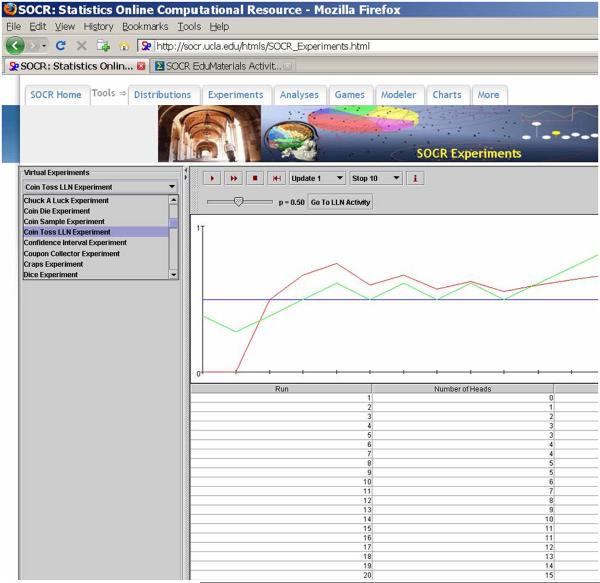
The SOCR LLN applet is designed as a meta-experiment (integrating functionality from SOCR Experiments and Distributions). In this applet, we provide the flexibility for choosing the number of trials and altering the probability of the event (in the meta-experiment of observing the frequencies of occurrence of the event in repeated independent trials). Figure 1 illustrates the main components of the applet interface. This applet may be accessed directly online at http://socr.ucla.edu/htmls/exp/Coin_Toss_LLN_Experiment.html (or from the main SOCR Experiments page: http://socr.ucla.edu/htmls/exp). There are tool-tips included for every widget in this applet. The tool-tips are pop-up information fields which describe interface features, and are activated by bringing the mouse over a component within the applet window. The control-toolbar of this applet, top of Figure 1, is included here as an insert . This toolbar contains the following experiment action control-buttons (left-to-right): running a single-step trial, running a multi-trial experiment, stopping of a multi-trial experiment, experiment resetting, frequency of updating the results table, number of trials to run (n), and an information dialog about the LLN experiment. Note that in the applet, the probability of a Head (p) and the number of experiments (n) are selected by the Probability-of-heads slider (defaulted to p=0.5) and the Sample-size/Stop-frequency drop-down list (defaulted to “Stop 10”), respectively.

Figure 1.

SOCR LLN APplet interface.

In addition to other SOCR libraries, this applet utilizes ideas, designs and functionality from the Rice Virtual Laboratory of Statistics (RVLS) and the University of Alabama Virtual Laboratories in Probability and Statistics (VirtualLabs).

2.2 SOCR LLN Activity

The SOCR LLN activity is available online (http://wiki.stat.ucla.edu/socr/index.php/SOCR_EduMaterials_Activities_LLN) and accessible from any Internet connected computer with Java-enabled web browser. The activity includes dynamic links to web resources on the LLN, interactive LLN demonstrations and relevant SOCR resources.

2.2.1 The first LLN experiment

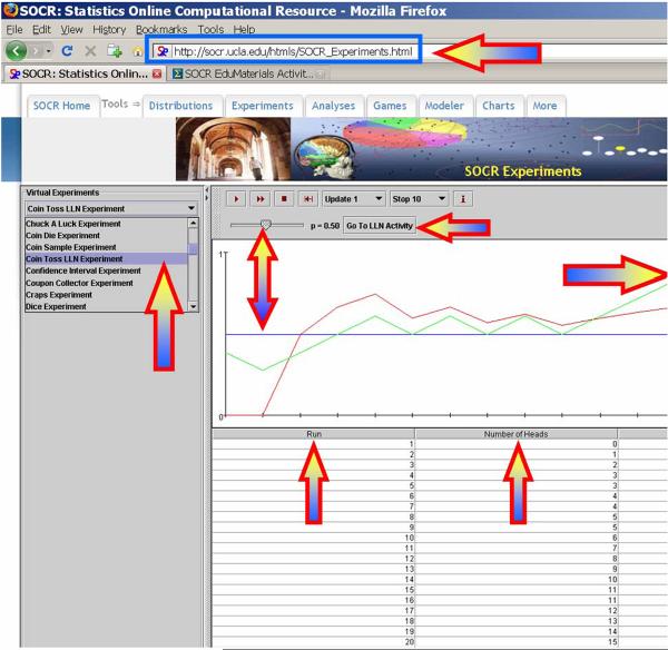
illustrates the statement and validity of the LLN in the situation of tossing (biased or fair) coins repeatedly, Figure 2. The arrows in Figure 2 point to the applet URL, and the main experimental controls – action-buttons (top), LLN experiment selection from the drop-down list (left), probability of a Head slider and graph-line (middle), and the headings of the results table (bottom). If H and T denote Heads and Tails, the probabilities of observing a Head or a Tail at each trial are 0 ≤ p ≤ 1 and 0 ≤ 1 – p ≤ 1, respectfully. The sample space of this experiment consists of sequences of H's and T's. For instance, an outcome may be {H,H,T,H,H,T,T,T,….}. If we toss a coin n times, the size of the sample-space is 2ⁿ, as the coin tosses are independent. The probability of observing 0 ≤ k ≤ n Heads in the n trials is governed by the Binomial Distribution and can be easily evaluated by the binomial density at k (e.g., http://socr.ucla.edu/htmls/SOCR_Distributions.html). In this experiment, we are interested in two random variables associated with this process. The first variable will be the proportion of Heads and the second will be the difference between the number of Heads and Tails in the n trials. Indeed, these two variables are chosen as they directly relate to the two most common LLN misconceptions (see section 1.4).

Figure 2.

SOCR LLN Activity: Snapshot of the first experiment.

To start the SOCR LLN Experiment go to http://socr.ucla.edu/htmls/exp/Coin_Toss_LLN_Experiment.html (note that the Coin Toss LLN Experiment is automatically selected in the drop-down list of experiments on the top-left). Now, select number of trials n=100 (Stop 100) and p=0.5 (fair-coin). Each time the user runs the applet, the random samples will be different, and the figures and results will generally vary. Using the Step () or Run () buttons will perform the experiment one or many times. The proportion of heads in the sample of n trials, and the difference between the number of Heads and Tails will evolve over time as shown on the graph and in the results table below. The statement of the LLN in this experiment reduces to the fact that as the number of experiments increases, the sample proportion of Heads (red curve) will approach the user-preset theoretical (horizontal blue line) value of p (in this case p=0.5). Changing the value of p and running the experiment interactively several times provides evidence that the LLN is invariant with respect to p.

In the SOCR LLN activity, the learner is encouraged to explore deeper the LLN properties by fixing a value of p and determining the sample-size needed to ensure that the sample-proportion stays within certain limits. One may also study the behavior of the curve representing the difference between the number of Heads and Tails (red curve) for various n and p values, or examine the convergence of the sample-proportion to the (preset) theoretical proportion. This is a demonstration of how the applet may be used to show theoretical concepts like convergence type and limiting behavior. The second misconception of the LLN (section 1.4) may be empirically dispelled by exploring the graph of the second variable of interest (the difference between the number of Heads and Tails). For all integers n, the independence of the (n+1)^st outcome from the results of the first n trials is also evident by the random behavior of the outcomes and the unpredictable and noisy shape of the graph of the normalized difference between the number of Heads and Tails. In fact, the number of Heads minus Tails difference is so chaotic, unstable and divergent that it can not be even plotted on the same scale as the plot of the Heads-to-Tails ratio.

We have defined an interesting normalization of the raw differences between the number of Heads and Tails to demonstrate the stochastic shape of this unstable variable. The normalized difference between the number of Heads and Tails in the graph is defined as follows: First, we let H_k and T_k represent the number of Heads and Tails, up to the current trial (k), respectively. Then we define the normalized difference

$$\mid \Vert H_k-T_k\Vert =p+\left(\frac{(1-p)H_k-p{T}_k}{\frac{2}{3}{\text{Max}}_k}\right),$$

where the maximum raw difference between the number of Heads and Tails in the first k trials is defined by

$${\text{Max}}_k=\underset{1{\le }_i{\le }_k}{\text{max}}\mid H_i-T_i\mid .$$

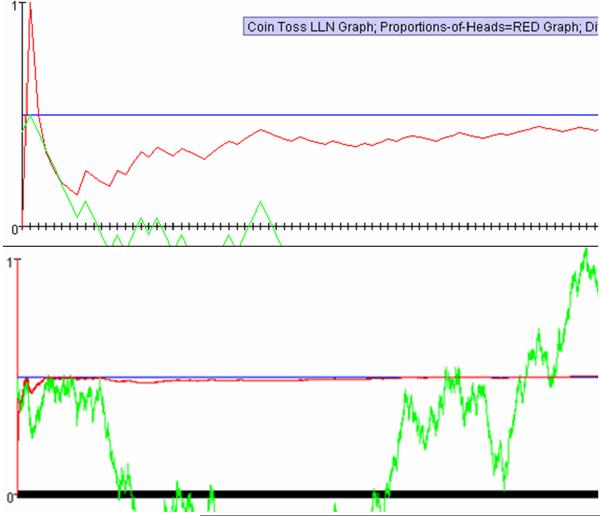
Since E((1 − p) H_k − pT_k) = 0, the expectation of the numerator is trivial, we know that the normalized difference will oscillate around p. Here, the denominator is introduced to scale the normalized difference and dampen the variance of this divergent process, which improves its graphical display. The normalized differences oscillate around the chosen p (the preset LLN limit of the proportion of Heads) and they are mostly visible within the graphing window alongside the graph of the Head-to-Tail proportion variable. However, the normalized difference does not have a well-defined finite expectation (Siegel, Romano, & Siegel, 1986). Figure 3 illustrates the symmetric, yet explosive and unstable nature of the variable representing the normalized difference between the number of Heads and Tails, $\mid \Vert H-T\Vert \mid$. Note the increase in the scale on the vertical line on the right hand side, as we increase from 100 (top panel) to 10,000 (bottom panel) experiments.

Figure 3.

Interactive applet demonstration of the two common LLN misconceptions. First, the outcome of each experiment is independent of the previous outcomes. Second, the variable representing the raw difference between the number of Heads and Tails is divergent, unstable and unpredictable. The top panel shows a simulation with only 100 trials. The bottom panel shows an outcome with 10,000 simulations. Notice the rapid convergence of the red curve (proportions), the expansion of the vertical scale on the right side and the vertical graph compression of the $\mid \Vert H-T\Vert \mid$ variable that follows with such a large increase in the number of trials.

2.2.2 The second LLN experiment

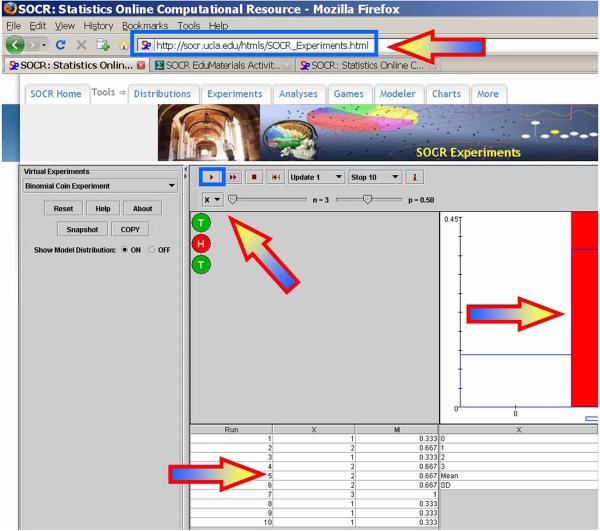
uses the Binomial coin applet to demonstrate that the (one-parameter) empirical and theoretical distributions of a random variable become more and more similar as the sample-size increases. Figure 4 shows the Binomial coin experiment (http://socr.ucla.edu/htmls/exp/Binomial_Coin_Experiment.html). Again, arrows and highlight-boxes identify the applet URL and main components (top to bottom): action control buttons, variable selection list, graph comparison between the model and empirical distributions, quantitative results table, and quantitative comparison between the theoretical and sample empirical distributions.

Figure 4.

SOCR LLN Activity: Snapshot of the second (Binomial coin) experiment.

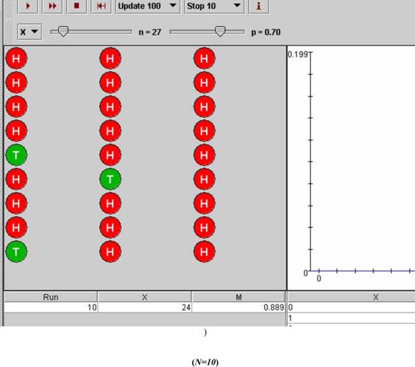
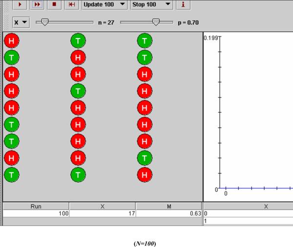
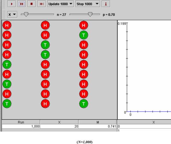
The user may select the number of coins (e.g., n=3) and probability of heads (e.g., p=0.5). Then, the right panel shows in blue color the model distribution (Binomial) of the Number of Heads (X). By varying the probability (p) and/or the number of coins (n), we see how these parameters affect the shape of the model distribution. As p increases, the distribution moves to the right and becomes concentrated at the right end (i.e., left-skewed). As the probability of a Head decreases, the distribution becomes right-skewed and centered in the left end of the range of X (0 ≤ X ≤ n). The LLN implies that if we were to increase the number of experiments (N), say from 10 to 100, and then to 1,000, we will get a better fit between the theoretical (Binomial) and empirical distributions. In particular, we get as a better estimate of the probability of a Head (p) by the sampling proportion of Heads $\left(\widehat{p}\right)$, cf. section 1.2. And this convergence is guaranteed for each p and each n (number of trials within a single experiment). Note that in this applet, the Binomial distribution parameters (n, p) are controlled by Number-of-coins (n) and Probability-of-heads (p) sliders, and the number of experiments we perform is selected by the Stop-frequency drop-down list in the control-button toolbar. Figure 5 illustrates this improved match of the theoretical (blue) and empirical (red) distribution graphs as the number of experiment (N) increases.

Figure 5.

Demonstration of the LLN using the Binomial coin experiment. As we increase the number of experiments (N) from 10 (top) to 100 (middle) and then to 1,000 (bottom), we observe a better match between the theoretical distribution (blue graph) and the empirical distribution (red graph). In this case, we used number of coin-tosses n=27 and p=P(H)=0.7. According to the LLN, the same behavior can be demonstrated for any choice of these Binomial parameters.

Similar improvements in the match of the theoretical and empirical distributions may be observed for many other processes modeled by one-parameter distributions using the other SOCR Experiments. For instance, in the Ball and Urn Experiment, where one may study the distribution of Y, the number of red balls in a sample of n balls (with or without replacement), we see similar LLN effects as the number of experiments (Stop-frequency selection) increases.

Another LLN illustration is based on the SOCR Poker experiment where one may be interested in how many trials are needed (on average) until a single pair of cards (same denomination) is observed. We can demonstrate the LLN by running the Poker experiment 100 times and recording the number of trials (5-card hands) containing a single pair (indicated by a value of V=1). Dividing this number by the total number of trials (100) we get a sample proportion of single-pair trials ($\widehat{p}$), which will approximate p, the theoretical probability of observing a single pair. The same experiment can be repeated with stopping criterion being set to V=1, instead of a specific (fixed) number of trials. Then, the (theoretical) expectation of the number of trials (n) needed to observe the first success (single-pair hand) is 1/p, as this is a Geometric process. This expectation can be approximated by the (empirical) number of trials ($\widehat{n}$) to observe the first single-pair hand. In this case, the LLN implies that the more experiments we perform, the closer the estimates of $\widehat{p}$ and $\widehat{n}$ to the theoretical values of their counterparts, p and n.

2.3 Applications

There are a number of applications of the LLN (DeHon, 2004; Rabin, 2002; Uhlig, 1996). The following two LLN applications demonstrate estimation of transcendental numbers for the two most popular transcendental numbers — π and e.

There are a number of equivalent definitions for the natural number e (http://en.wikipedia.org/wiki/E_(mathematical_constant)). One of these is

$$e=\underset{n\to \infty }{\mathit{lim}}{\left(1+\frac{1}{n}\right)}^n.$$

Using simulation, the number e may be estimated by random sampling from a continuous Uniform distribution on (0, 1). Suppose X₁,X₂, …,X_k are drawn from a uniform distribution on (0, 1) and define

$$U=\underset{k}{\text{argmin}}\{X_1+X_2+\dots +X_k>1\}.$$

It turns out that the expected value E(U)=e ≈ 2.7182, (Russell, 1991). Therefore, by the LLN, taking averages of U₁, U₂, U₃, …, U_n, where each U_i is computed from a random sample

$$\{X_1,X_2,\dots ,X_{k_4}\}$$

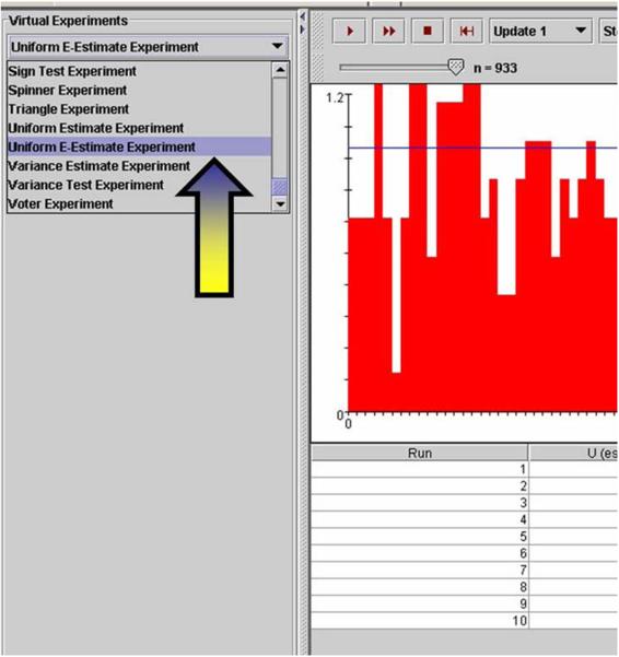
as described above, will provide a more accurate estimate of the natural number e (as n →∞). The SOCR E-Estimate Experiment (http://wiki.stat.ucla.edu/socr/index.php/SOCR_EduMaterials_Activities_Uniform_E_EstimateExperiment) provides an activity with the complete details of this simulation and the corresponding Uniform E-Estimate Experiment applet http://socr.ucla.edu/htmls/exp/Uniform_E-Estimate_Experiment.html. The experiment illustrates hands-on this stochastic approximation of e by random sampling. Figure 6 shows the graphical user interface behind this simulation. The arrows in Figure 6 point to the applet selection from the drop-down list of applets (left), the results table containing the outcome of 10 simulations (middle) and the (theoretical and empirical) estimate of the bias and precision (MSE) of the approximation of e by random sampling (right). The graph panel in the middle shows the values of the Uniform(0,1) sample, X₁,X₂, …,X_k, used to compute the values of U. For instance, if you set n=1, the graph will typically show 2 or 3 Uniform random variables (the smallest number of variables whose sum exceeds 1). For higher n, the applet shows the sample frequencies and computes the averages of the smallest numbers, for all collections of variables whose sum exceeds 1. And this average is used to estimate e. Notice how the quality of the estimate increases (bias goes to zero) as n increases. In Figure 6, n=933 and the bias is −0.018. One can also rapidly increase the estimator accuracy by repeating the experiment 100 or 1,000 times (by repeating the experiment 100 or 1,000 times (by setting “Stop 1,000” in the control bar).

Figure 6.

SOCR Uniform E-Estimate applet illustrating the stochastic approximation of e by random sampling from Uniform(0,1) distribution.

The SOCR Buffon's Needle Experiment provides a similar approximation to π, which represents the ratio of the circumference of a circle to its diameter, or equivalently, the ratio of a circle's area to the square of its radius in 2D Euclidean space. The LLN provides a foundation for an approximation of π using repeated independent virtual drops of needles on a tiled surface by observing if the needle crosses a tile grid-line. For a tile grid of size 1, the odds of a needle-line intersection are $\frac{2}{n}\approx 0.63662$, (Schroeder, 1974). In practice, to estimate π from a number of needle drops (N), we take the reciprocal of the sample odds-of-intersection. The complete details of this application are also available online at http://wiki.stat.ucla.edu/socr/index.php/SOCR EduMaterials_Activities_BuffonNeedleExperiment and http://socr.ucla.edu/htmls/SOCR_Experiments.html.

3. Discussion and Utilization

3.1 How to use the pair of SOCR LLN applets and activities in the classroom

There is no single best way to use of these resources in the classroom. An instructor must always fine-tune these materials to their specific course curriculum. There are a number of ways that we have experimented with these materials in the past. One may begin either with more illustrative empirical demonstrations that build students' intuition for the subsequent symbolic mathematical formulation of the experimentally observed properties. Instructors may also choose to explain the LLN mathematical formalism first, and then provide supporting empirical evidence using the SOCR LLN simulations to solidify students' comprehension of the LLN. Open discussions with learners, involving the applet usage, LLN properties, examples and counterexamples, provoke significantly higher participation and demonstrate a marked increase of students' interest in the subject. Instructors may build complexity in these demonstrations based on students' responses, attentiveness and comprehension. A homework assignment that reinforces these LLN principles is appropriate in many cases and may improve knowledge retention.

One specific approach for teaching the concept of the LLN in various classes is to follow the SOCR LLN activity step-by-step. Instructors would typically begin by presenting one or two motivational examples. Then, as appropriate, the instructor may discuss the formal statement(s) of the LLN, and perform several simulations using the LLN applet. Students may then be given 5–10 minutes to explore the hands-on section of the LLN Wiki activity on their own by following the directions and answering the questions. Instructors must follow up with a question-and-answer period to ensure all students understand the mechanics, purpose and applications included in the LLN activities. Finally, it is appropriate to encourage an open classroom discussion, utilizing the LLN applet, explaining the two LLN misconceptions.

3.2 What is unique about the SOCR LLN Activity?

There are two aspects of the SOCR LLN activity and applets that we believe are of most use to instructors and learners alike. The first one is the broad spectrum of experiments employed in the demonstration of the theoretical and empirical properties, as well as applications of the LLN. These materials demonstrate the law of large numbers in terms of proportions and averages, for a variety of processes modeled by different distributions and point out the main misunderstandings of the LLN. The second beneficial aspect of these resources is the interactive nature and full user control over parameter choices, which facilitates intuition building, empirical motivation and result validation of the LLN for novice learners (e.g., disproving empirically impossible probabilities like P(Head)=0.1 for a repeated fair coin toss experiment).

3.3 Other SOCR Activities

The SOCR resource has continuously been developing other similar hands-on activities. These are paired with one or more SOCR applets and typically illustrate one possible approach for demonstrating a probability or statistics property via a SOCR distribution, experiment, analysis, graphing or modeling applet. Most of the general topics covered in lower and upper division probability theory or statistical inference courses already have available one or several SOCR Wiki activities (http://wiki.stat.ucla.edu/socr/index.php/SOCR_EduMaterials). There are many other instances of SOCR activities covering the distribution, analyses, experiments, graphs and modeler applets. Finally, there are also some SOCR applets and activities, which may be used in more advanced undergraduate and graduate level classes, e.g., central limit theorem, mixture modeling, expectation maximization, Fourier and wavelet signal representation, etc.

References

- ARTIST 2006 https://app.gen.umn.edu/artist/
- BlackBoard 2006 http://www.blackboard.com/
- Blasi L, Alfonso B. Increasing the transfer of simulation technology from R&D into school settings: An approach to evaluation from overarching vision to individual artifact in education. Simulation Gaming. 2006;37:245–267. [Google Scholar]
- Brescia W, Miller M. What's it worth? The perceived benefits of instructional blogging. Electronic Journal for the Integration of Technology in Education. 2006;5:44–52. [Google Scholar]
- ClickTV 2006 http://blog.click.tv/
- DeHon A. Nano, Quantum and Molecular Computing. Kluwer Academic Publishers; Boston, MA: 2004. Law of large numbers system design. [Google Scholar]
- Dinov I. SOCR: Statistics Online Computational Resource: socr.ucla.edu. Statistical Computing & Graphics. 2006a;17:11–15. doi: 10.18637/jss.v016.i11. [DOI] [PMC free article] [PubMed] [Google Scholar]
- Dinov I. Statistics Online Computational Resource. Journal of Statistical Software. 2006b;16:1–16. doi: 10.18637/jss.v016.i11. [DOI] [PMC free article] [PubMed] [Google Scholar]
- Dinov I, Sanchez J, Christou N. Pedagogical Utilization and Assessment of the Statistic Online Computational Resource in Introductory Probability and Statistics Courses. Journal of Computers & Education. 2006c doi: 10.1016/j.compedu.2006.06.003. in press. [DOI] [PMC free article] [PubMed] [Google Scholar]
- Dinov I, Christou N, Sanchez J. Central Limit Theorem: New SOCR Applet and Demonstration Activity. Journal of Statistical Education. 2008;16:1–12. doi: 10.1080/10691898.2008.11889560. [DOI] [PMC free article] [PubMed] [Google Scholar]
- Durrett R. Probability: Theory and Examples. Duxbury Press; 1995. [Google Scholar]
- Forster P. Assessing technology-based approaches for teaching and learning mathematics. International Journal of Mathematical Education in Science and Technology. 2006;37:145–164. DOI: 10.1080/00207390500285826. [Google Scholar]
- Garfield J. How students learn statistics. International Statistical Review. 1995;3:25–34. [Google Scholar]
- IVTWeb 2006 www.ivtweb.com/
- Judd K. The law of large numbers with a continuum of IID random variables. Journal of Economic Theory. 1985;35:19–25. [Google Scholar]
- Leslie M. Statistics Starter Kit. Science. 2003;302:1635. [Google Scholar]
- LetsTalk LetsTalk. 2006 http://duber.com/LetsTalk.
- Lunsford M, Holmes-Rowell G, Goodson-Espy T. Classroom Research: Assessment of Student Understanding of Sampling Distributions of Means and the Central Limit Theorem in Post-Calculus Probability and Statistics Classes. Journal of Statistics Education. 2006;14 [Google Scholar]
- Mishra P, Koehler M. Technological Pedagogical Content Knowledge: A Framework for Teacher Knowledge. Teachers College Record. 2006;108:1017–1054. doi:10.1111/j.1467-9620.2006.00684.x. [Google Scholar]
- MOODLE 2006 http://moodle.org/
- PBSBlog 2006 http://www.pbs.org/teachersource/learning.now.
- Rabin M. Inference By Believers in the Law of Small Numbers. Quarterly Journal of Economics. 2002;117:775–816. [Google Scholar]
- Russell KG. Estimating the Value of e by Simulation. The American Statistician. 1991;45:66–68. [Google Scholar]
- RVLS http://www.ruf.rice.edu/%7Elane/rvls.html.
- SAKAI http://www.sakaiproject.org/
- Schroeder L. Buffon's needle problem: An exciting application of many mathematical concepts. Mathematics Teacher. 1974;67:183–186. [Google Scholar]
- Siegel J, Romano P, Siegel A. Counterexamples in Probability and Statistics. CRC Press; 1986. [Google Scholar]
- SOCRWiki . SOCR Wiki Resource. UCLA; 2006. http://wiki.stat.ucla.edu/socr. [Google Scholar]
- Symanzik J, Vukasinovic N. Teaching an Introductory Statistics Course with CyberStats, an Electronic Textbook. Journal of Statistics Education. 2006;14 [Google Scholar]
- TCEXAM TCExam Testbank http://sourceforge.net/projects/tcexam/
- Tversky A, Kahneman D. Belief in the law of small numbers. Psychological Bulletin. 1971;76:105–110. [Google Scholar]
- UCLAVOH 2006 http://voh.chem.ucla.edu/
- UCLAX UCLA Extension Online Courses. UCLA Extension. 2006 http://www.uclaextension.edu.
- Uhlig H. A Law of Large Numbers for Large Economies. Economic Theory. 1996;8:41–50. [Google Scholar]
- VirtualLabs http://www.math.uah.edu/stat/
- WebWork http://www.opensymphony.com/webwork.
- WikiBooks 2006 http://en.wikibooks.org/wiki/Blended_Learning_in_K-12.