Solution of the nonlinear elasticity imaging inverse problem: The incompressible case

Abstract

We have recently developed and tested an efficient algorithm for solving the nonlinear inverse elasticity problem for a compressible hyperelastic material. The data for this problem are the quasi-static deformation fields within the solid measured at two distinct overall strain levels. The main ingredients of our algorithm are a gradient based quasi-Newton minimization strategy, the use of adjoint equations and a novel strategy for continuation in the material parameters. In this paper we present several extensions to this algorithm. First, we extend it to incompressible media thereby extending its applicability to tissues which are nearly incompressible under slow deformation. We achieve this by solving the forward problem using a residual-based, stabilized, mixed finite element formulation which circumvents the Ladyzenskaya–Babuska–Brezzi condition. Second, we demonstrate how the recovery of the spatial distribution of the nonlinear parameter can be improved either by preconditioning the system of equations for the material parameters, or by splitting the problem into two distinct steps. Finally, we present a new strain energy density function with an exponential stress-strain behavior that yields a deviatoric stress tensor, thereby simplifying the interpretation of pressure when compared with other exponential functions. We test the overall approach by solving for the spatial distribution of material parameters from noisy, synthetic deformation fields.

1. Introduction

It is well known that many solid tumors, such as breast and prostate tumors, are stiffer than healthy glandular tissue. This fact has been used for some time to detect tumors using finger palpation. In the last one to two decades, it has lead to the development of a group of techniques, collectively referred to as elastography or elasticity imaging (see [1–5] for reviews), that focus on generating images of tissue stiffness, or quantities that are indicative of its distribution (such as strain). More recently, it has been observed that while both benign and malignant tumors are stiff, the latter appear to stiffen with strain at a faster rate than either the background tissue, or benign tumors [6–8]. While it has not yet been shown conclusively why this happens, it appears likely it is due to the structure of collagen fibers. In benign tumors they appear to be significantly coiled whereas in malignant tumors they are straighter and almost rod-like [9,10]. The fibers tend to uncoil, or straighten, with applied strain. Thus it would appear likely that in a malignant tumor, the fibers would start to contribute to the strength of the tissue at smaller strains than in benign tumors. Regardless of precisely why it happens, the strong strain hardening behavior of malignant tumors leads to the intriguing possibility of diagnosing cancerous tumors on the basis of images of nonlinear tissue behavior. Evidence supporting this possibility has recently been presented by O'Hagan and Samani [11], who address precisely this question in an experimental study of 44 ex vivo breast tumors.

In quasi-static elasticity imaging the region of interest is viewed using conventional imaging techniques, usually ultrasound, while it is slowly compressed. Images recorded during the compression are then used to determine the displacement field within the tissue. Using this approach displacement fields with overall compressive strains that are as high as 15% have been evaluated. At these strains, the nonlinear behavior of tissue is likely to play an important role. This data may therefore be useful in reconstructing images of nonlinear tissue material properties once the associated inverse problem is solved. The solution of this inverse problem is the focus of this paper.

In preceding work [12,8] we described a strategy for solving this problem for a compressible medium (or more precisely, for an incompressible medium in plane stress.) We modeled the solid as a hyperelastic material with an exponential stress–strain response based on the Veronda–Westmann model [13]. We posed the inverse problem as a minimization problem and sought the distribution of material parameters that yields the displacement fields that best match the measured displacement fields. We solved this problem using a gradient based quasi-Newton algorithm. Two key features leading to the high computational efficiency of the method were evaluation of the gradient using the adjoint equations and utilization of a novel continuation strategy in material parameters. We tested this approach on synthetic noisy data as well as clinical data.

In this paper we present several extensions to our earlier approach. First we extend our analysis to incompressible media, thereby making it feasible to model incompressible tissue in plane strain in two-dimensions or in three-dimensions. We accomplish this by solving the forward problems at each iteration using a residual-based, stabilized, mixed finite element formulation, thereby circumventing the LBB condition [14,15]. This approach was developed in [16,17] and applied to linear elastic materials and then to Neo–Hookean materials. In this paper we consider its application to solids with material nonlinearity.

Second, we propose and test two strategies to improve the recovery of the nonlinear parameter in our reconstructions, without adversely affecting the recovery of the linear modulus. In [12] it was observed that the recovery of the nonlinear parameter is not as accurate as that of the linear shear modulus. We have since recognized that one reason for this is the lower sensitivity of the displacement field to the nonlinear parameter, even for the deformation fields measured at large values of overall strain. In order to alleviate this problem we propose and test two strategies. First, we simply rescale the nonlinear parameter by a fixed constant, effectively preconditioning the system of equations with a diagonal preconditioner. Second we decouple the problem for the nonlinear parameter from the problem from the linear parameter. The deformation fields at small values of strain carry no information about the nonlinear parameter. Thus the linear parameter may be estimated using these fields. Once it is known, the nonlinear parameter may be estimated using the large deformation fields.

Finally, we also adopt a new strain energy density function that, like the functions due to Blatz et al. [18] and Veronda and Westmann [13], stipulates an exponential stress–strain behavior. Unlike these models, however, it yields a stress contribution that is purely deviatoric. This simplifies the interpretation of pressure in the stress–strain relation.

The format of the remainder of this paper is as follows: In Section 2, we describe the forward elasticity problem and its discretization. This includes the new strain energy density function and the stabilization strategy for the finite element solution of the problem. In Section 3 we describe the inverse problem and our solution. This includes the use of the adjoint equations to efficiently compute the gradient vector. We remark that we derive the adjoint of the fully discretized forward problem. This ensures that the computed gradient of the discrete objective function is exact up to numerical roundoff. In Section 4, we consider numerical examples that test our approach for solving the forward and the inverse problems. We also motivate and describe rescaling and staggered solution strategies that improve the performance of the algorithm in recovering the nonlinear parameter. We end with conclusions in Section 5.

2. Nonlinear forward elasticity problem

The material response is modelled with a hyperelastic model. In hyperelasticity, the existence of a strain energy density function is assumed from which a constitutive relation between stress and strain is derived. The total energy that is needed to deform the body is only dependent on the initial and the end state, that is, the state of the body is independent of the loading path.

Throughout this paper equations are written in the reference configuration and tensors and vectors are denoted by bold letters.

2.1. Strong form

The strong form is given in general terms without any specification of the stress–strain relation. This is specified in detail in Section 2.4. The strong form is: Find the displacement field u and the pressure p such that:

$$\nabla \cdot (\mathit{\text{FS}})=\mathbf{0}\text{in}{\Omega }_0,$$ (1)

$$\mathit{\text{u}}=\mathit{\text{g}}\text{on}{\Gamma }_g,$$ (2)

$$\mathit{\text{FS}}\cdot \mathit{\text{n}}=\mathit{\text{h}}\text{on}{\Gamma }_h$$ (3)

with the incompressibility constraint:

$$J-1=0,\text{in}{\Omega }_0.$$ (4)

As mentioned above, this problem statement must be augmented by the stress–strain relation to specify the stress in terms of the deformation. This discussion is postponed until Section 2.4.

In the equations above Ω₀ is the reference configuration or reference domain. Eqs. (2) and (3) define the Dirichlet and Neumann boundary conditions, respectively, where the displacement data g is prescribed on Γ_g and the traction data h is prescribed on Γ_h. The following restrictions are given on Γ_g and ${\Gamma }_h:\partial {\Omega }_0=\overline{{\Gamma }_g\cup {\Gamma }_h}$ defines the closed boundary of the domain and Γ_g ∩ Γ_h = θ. F = ∇ϕ is the deformation gradient associated with the transformation ϕ that maps the material points X into the current locations x = ϕ(X). The displacement field can be determined from ϕ as u = ϕ − X. The gradient operator ∇ in the equations above is defined with respect to the material coordinates. The incompressibility constraint in Eq. (4) enforces that the Jacobian or determinant of the deformation gradient J = detF = 1, so that there is no change of volume. Further, n is the unit outward normal vector along the boundary and S is the second Piola–Kirchhoff stress tensor defined as:

$$\mathit{\text{S}}=-pJ{\mathit{\text{C}}}^{-1}+2\frac{\partial W}{\partial \mathit{\text{C}}}.$$ (5)

Here p is the pressure and W is the strain energy density function that depends on the invariants of the Cauchy–Green strain tensor C = F^TF.

2.2. Weak form

The weak form can be derived easily from the strong form by multiplying Eq. (1) with a vector test function, integrating-by-parts over the reference domain, and utilizing the traction boundary condition. The incompressibility constraint is multiplied by another scalar test function and integrated over the reference domain. The weak form is given by: Find U ≡ [u, p] ∈ × such that

$$\mathcal{A}(\mathit{\text{W}},\mathit{\text{U}};\mathit{\text{β}})-{(\mathit{\text{w}},\mathit{\text{h}})}_{{\Gamma }_h}=0,\forall \mathit{\text{W}}\equiv [\mathit{\text{w}},q]\in \mathcal{\text{V}}\times \mathcal{\text{P}},$$ (6)

where

$$\mathcal{A}(\mathit{\text{W}},\mathit{\text{U}};\mathit{\text{β}})={\int }_{{\Omega }_0}{w}_{k,\alpha }{F}_{k\beta }{S}_{\alpha \beta }d{\Omega }_0+{\int }_{{\Omega }_0}(J-1)qd{\Omega }_0,$$ (7)

$${(\mathit{\text{w}},\mathit{\text{h}})}_{{\Gamma }_{\mathit{\text{h}}}}={\int }_{{\Gamma }_h}\mathit{\text{w}}\cdot \mathit{\text{h}}d{\Gamma }_0.$$ (8)

The function spaces , , and are defined as:

$$\mathcal{V}=\{\mathit{\text{w}}\mid w_i\in H^1({\Omega }_0);w_i=0\text{on}{\Gamma }_g\},$$ (9)

$$\mathcal{S}=\{\mathit{\text{u}}\mid u_i\in H^1({\Omega }_0);u_i=g_i\text{on}{\Gamma }_g\},$$ (10)

$$\mathcal{\text{P}}\subseteq L_2({\Omega }_0).$$ (11)

2.3. Stabilization of the discretized mixed formulation

The weak form (6) may be discretized by selecting finite dimensional spaces ^h ⊂ , ^h ⊂ and ^h ⊂ and using Galerkin's approach. This leads to a nonlinear algebraic problem for the displacement and pressure degrees of freedom that may be solved using the Newton–Raphson method. When equal order polynomials are used for the displacement and pressure trial solutions and weighting functions, the resulting linearized system does not satisfy the LBB conditions [14,15]. The linear system has the form

$$\left(\begin{array}{cc}{\mathbf{\text{K}}}_{11}& {\mathbf{\text{K}}}_{12}\\ {\mathbf{\text{K}}}_{21}& \mathbf{0}\end{array}\right)\left(\begin{array}{c}\mathbf{\text{u}}\\ \mathbf{\text{p}}\end{array}\right)=(\mathit{\text{RHS}})$$ (12)

which is typical of a saddle point problem. The difficulty lies in the matrix K₁₂ which does not satisfy the discrete inf–sup conditions. This deficiency manifests itself as spurious oscillations in pressure modes and locking in the displacement field. Over the years several remedies have been proposed to tackle this problem. These include selective reduced integration schemes, Taylor–Hood elements that employ different displacement and pressure interpolation functions that satisfy the LBB conditions, the B-bar approach [19], the enhanced strain approach [20] and stabilized finite element methods [16,17].

In this paper, following [16,17] we have utilized an equal order stabilized finite element method based on the streamline upwind (SUPG) approach. In this approach the Galerkin form is appended with additional terms that are driven by the residual of the original equations. These terms stabilize the method while retaining its consistency. In particular, the weak form is given by: Find U^h ≡ [u^h, p^h] ∈ ^h × ^h such that

$$\begin{array}{l}\mathcal{A}({\mathit{\text{W}}}^h,{\mathit{\text{U}}}^h;\mathit{\text{β}})+ℛ({\mathit{\text{W}}}^h,{\mathit{\text{U}}}^h;\mathit{\text{β}})={({\mathit{\text{w}}}^h,\mathit{\text{h}})}_{{\Gamma }_h}\\ \forall {\mathit{\text{W}}}^h\equiv [{\mathit{\text{w}}}^h,q^h]\in {\mathcal{\text{V}}}^h\times {\mathcal{\text{P}}}^h,\end{array}$$ (13)

where the stabilization term is given by

$$ℛ({\mathit{\text{W}}}^h,{\mathit{\text{U}}}^h;\mathit{\text{β}})=-\sum _{e=1}^{n_{el}}{(\tau \nabla \cdot (\mathit{\text{FS}}),{\mathit{\text{F}}}^{-T}\nabla q^h)}_{{\Omega }_0^e}.$$ (14)

In the equation above the subscript ${(\cdot ,\cdot )}_{{\Omega }_0^e}$ is the $L_2({\Omega }_0^e)$ inner product evaluated in the interior of the eth element and

$$\tau =\frac{\alpha h^2}{2\mu }.$$ (15)

We note that in the stabilization term the integration is performed over the element interiors and summed over all elements. The integrand consists of the scalar product of the gradient of the weighting function with the residual of the momentum equation. When converging to the exact solution, this term becomes zero, and the consistency of the method is retained. The stabilization parameter τ in Eq. (15) consists of a factor α ≈ 1/2, the shear modulus μ, and the characteristic element length h which would be the diameter of the outer circle for triangular elements. For further information about the stabilized mixed formulation the reader is referred to [21].

Following [17], the stabilization term may be simplified as follows

$$\begin{array}{ll}ℛ({\mathit{\text{W}}}^h,{\mathit{\text{U}}}^h;\mathit{\text{β}})\hfill & =-\sum _{e=1}^{n_{el}}\left({\left(\tau \nabla \cdot \left(2\mathit{\text{F}}\frac{\partial W}{\partial \mathit{\text{C}}}\right),{\mathit{\text{F}}}^{-T}\nabla q^h\right)}_{{\Omega }_0^e}+{\left(\tau \nabla \cdot \left(2p^h\mathit{\text{F}}\frac{\partial J}{\partial \mathit{\text{C}}}\right),{\mathit{\text{F}}}^{-T}\nabla q^h\right)}_{{\Omega }_0^e}\right)\hfill \\ & =\sum _{e=1}^{n_{el}}{\left(\tau \nabla \cdot (p^{h}J{\mathit{\text{F}}}^{-T}),{\mathit{\text{F}}}^{-T}\nabla q^h\right)}_{{\Omega }_0^e}\hfill \\ & =\sum _{e=1}^{n_{el}}{\left(\tau J{\mathit{\text{F}}}^{-T}\nabla p^h,{\mathit{\text{F}}}^{-T}\nabla q^h\right)}_{{\Omega }_0^e}.\hfill \end{array}$$ (16)

To arrive at the first equality of (16) we have used (5) in (14). To arrive at the second equality we note that since we are working with linear triangular elements, the deformation gradients and hence all strains and stresses (except pressure) are constant within an element, and therefore their divergence is zero. This means that the first term on the right hand side of the first equality is zero. To simplify the second term we have utilized $\frac{\partial J}{\partial \mathbf{\text{C}}}=\frac{1}{2}{J\mathit{\text{C}}}^{-1}$. Finally to arrive at the last line we have made use of the Piola identity, ∇·(JF^−T) = 0.

The matrix system obtained after linearizing the stabilized formulation has the structure

$$\left(\begin{array}{cc}{\mathbf{\text{K}}}_{\mathbf{11}}& {\mathbf{\text{K}}}_{\mathbf{12}}\\ {\mathbf{\text{K}}}_{\mathbf{21}}& {\mathbf{\text{K}}}_{\mathbf{22}}\end{array}\right)\left(\begin{array}{c}\mathbf{\text{u}}\\ \mathbf{\text{p}}\end{array}\right)=(\mathit{\text{RHS}}),$$ (17)

where the submatrix K₂₂ is positive definite. This matrix system does not correspond to a saddle point problem, and its stability can be assessed by examining the coercivity of the method, which can be proved under certain restrictions. Thus when working with stabilized methods the LBB conditions for the incompressibility constraint may be circumvented.

2.4. Strain energy density function

A generic trend in the stress–strain relation of soft tissues is a gradual stiffening with applied strain [7,6,22,13]. Several writers have modeled this stiffening with an exponentially stiffening strain energy function. (See, e.g. [18,13] and the review focusing on arterial walls, [23].) Here we consider a modification of a model due to Blatz and coworkers [18]. The modification made here is to replace the appearance of I₁ with J^−2/3I₁. This change renders the elastic energy contribution purely deviatoric, which is particularly appropriate for modeling incompressible materials. Thus, the strain energy function used here is:

$$W=\frac{\mu }{2\gamma }\left(e^{\gamma \left(J^{-\frac{2}{3}}{I}_1-3\right)}-1\right).$$ (18)

Here μ is the shear modulus at zero strain, γ is a nonlinear parameter that determines the nonlinearity of the material response, and I₁ = trace (C) is the first principal invariant of the Cauchy Green tensor. This strain energy function has several advantages in this application. First it is capable of modeling the observed exponential stiffening of soft tissues. Second, it contains only two material parameters to evaluate, μ and γ. Third, the material parameters have clear, distinct, physical interpretations: μ governs the small strain behavior independent of the value of γ, while γ controls the exponential stiffening, independent of μ. The respective roles of these two parameters may be most easily seen in uniaxial tension for small strains. In this case, the stress–strain relation may be approximated by:

$$\sigma \approx 3\mu \varepsilon exp[3\gamma {\varepsilon }^2]\text{for}\varepsilon \ll 1.$$ (19)

Here, ε = λ − 1 is the linearized strain measure, and σ is the Cauchy stress.

The full nonlinear stress–strain behavior in uniaxial tension is given by the equation:

$$\sigma =\mu \left({\lambda }^2-\frac{1}{\lambda }\right)e^{\gamma \left({\lambda }^2+\frac{2}{\lambda }-3\right)},$$ (20)

where σ is the uniaxial Cauchy stress and λ is the stretch.

We plot the stress-stretch curve in Fig. 1(a) for a fixed shear modulus value of 1 and consider different values of the nonlinear parameter γ ranging from 1 to 11. At γ = 1 the stress-stretch curve is not significantly nonlinear. With increasing values of γ the nonlinearity of the material response increases noticeably.

Fig. 1.

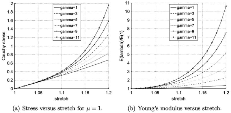
Nonlinear exponential behavior of the new strain energy density function.

In order to demonstrate the effect of the nonlinear parameter on the relative stiffening of the material with increasing strain we consider the ratio of the Young's modulus at a stretch λ to the Young's modulus at λ = 1. This ratio is given by

$$\frac{E(\lambda )}{E(\lambda =1)}=\frac{1}{3}{e}^{\gamma \left({\lambda }^2+\frac{2}{\lambda }-3\right)}[2\lambda +{\lambda }^{-2}+\gamma (2{\lambda }^3+2{\lambda }^{-3}-4)].$$ (21)

Right away we note that this ratio is independent of the shear modulus μ and depends only on the parameter γ. Fig. 1(b) shows variation of this ratio as a function of stretch for different values of γ. We note an exponential strain hardening whose extent is determined by the nonlinear parameter γ.

Returning now to the general 3D case, we use this definition for the strain energy density function in (5), to find the second Piola–Kirchhoff stress is given by

$$\mathit{\text{S}}=-pJ{\mathit{\text{C}}}^{-1}+\mu J^{-\frac{2}{3}}\left(\mathit{\text{I}}-\frac{1}{3}{I}_1{\mathit{\text{C}}}^{-1}\right)e^{\gamma \left(J^{-\frac{2}{3}}{I}_1-3\right)}$$ (22)

and the Cauchy stress σ is given by

$$\mathit{\text{σ}}=-p\mathit{\text{I}}+\mu J^{-\frac{5}{3}}\left({\mathit{\text{FF}}}^T-\frac{1}{3}{I}_1\mathit{\text{I}}\right)e^{\gamma \left(J^{-\frac{2}{3}}{I}_1-3\right)}.$$ (23)

Using the equation above it is easily verified that $\frac{\text{trace}(\mathbf{\sigma })}{3}=-p$, as expected for an incompressible medium. The material tangent corresponding to this strain energy density function is

$$\begin{array}{ll}{\mathcal{C}}_{\mathit{\text{ijkl}}}\hfill & =2\frac{\partial S_{ij}}{\partial C_{kl}}=4\frac{{\partial }^{2}W}{\partial C_{ij}\partial C_{kl}}-2\frac{\partial }{\partial C_{kl}}(pJ{C}_{ij}^{-1})\hfill \\ & =2\mu e^{\gamma \left(J^{-\frac{2}{3}}{I}_1-3\right)}\left(\gamma L_{ij}{L}_{kl}-\frac{1}{3}{C}_{kl}^{-1}{L}_{ij}+{\mathcal{\text{D}}}_{\mathit{\text{ijkl}}}-p{ℰ}_{\mathit{\text{ijkl}}}\right),\hfill \end{array}$$ (24)

where

$$L_{ij}=J^{-\frac{2}{3}}\left(-\frac{1}{3}{I}_1{C}_{ij}^{-1}+{\delta }_{ij}\right),$$ (25)

$${\mathcal{\text{D}}}_{\mathit{\text{ijkl}}}=-\frac{1}{3}{J}^{-\frac{2}{3}}\left({\delta }_{kl}{C}_{ij}^{-1}+\frac{1}{2}{I}_1(C_{ik}^{-1}{C}_{jl}^{-1}+C_{il}^{-1}{C}_{jk}^{-1})\right),$$ (26)

$${ℰ}_{\mathit{\text{ijkl}}}=J\left(C_{ij}^{-1}{C}_{kl}^{-1}+C_{ik}^{-1}{C}_{jl}^{-1}+C_{il}^{-1}{C}_{jk}^{-1}\right).$$ (27)

3. Nonlinear inverse elasticity problem

The solution of the inverse elasticity problem for compressible materials was discussed in detail in [12]. For the incompressible case discussed in this paper we adopt the same overall approach. In addition we introduce several new features that account for the incompressibility constraint and improve the performance of the method. In particular:

1. In solving the forward problem we have made use of stabilized finite element methods to handle the incompressibility constraint (see Section 2.3).

2. We have developed and implemented a modified version of the Blatz strain energy density function that ensures that the elastic part of the Cauchy stress is deviatoric (see Section 2.4).

3. We have consistently accounted for the stabilization terms in deriving the equations for the adjoint fields. This is described below in Section 3.2.

4. We have improved the reconstructions for the nonlinear parameter by recognizing that its contribution to the gradient tends to be smaller than the contribution from the shear modulus. These approaches are discussed in Sections 4.3 and 4.5.

The inverse problem is solved iteratively by minimizing an objective function under the constraint that the predicted displacement fields satisfy the forward problem. There is a wide range of methods that may be used to perform this minimization. Some, like genetic algorithms, require only values of the objective function, while others require first order or second order derivatives of the objective function. In this paper we work with a quasi-Newton method which requires only the first order derivatives of the objective function and constructs an approximate Hessian from these. In particular we use the low memory BFGS algorithm described in [24]. We evaluate the gradient efficiently using the adjoint equations.

3.1. Inverse problem statement

The inverse problem is stated as follows: Given n_meas measured displacement fields ${\mathit{\text{u}}}_{\mathit{\text{meas}}}^1,\dots ,{\mathit{\text{u}}}_{\mathit{\text{meas}}}^{{\mathit{\text{n}}}_{\mathit{\text{meas}}}}$, find the material properties β = [β₁, β₂, …, β_Nβ] such that the objective function

$$\pi =\frac{1}{2}\sum _{i=1}^{n_{\mathit{\text{meas}}}}{w}_i{\Vert \mathit{\text{T}}{\mathit{\text{u}}}^i-\mathit{\text{T}}{\mathit{\text{u}}}_{\mathit{\text{meas}}}^i\Vert }_0^2+\frac{1}{2}\sum _{j=1}^{N_{\beta }}{\alpha }_{j}R({\beta }_j)$$ (28)

is minimized under the constraint that the predicted displacement fields uⁱ satisfy the equations of equilibrium (1)–(4)).

For the material model we have selected, N_β = 2, with β₁ = μ and β₂ = γ, and recall that μ denotes the shear modulus at zero strain and γ denotes the nonlinear stiffening parameter. In Eq. (28) the first term is the displacement matching term and is a measure of how close the measured displacement field is to the ith predicted displacement field uⁱ in the L₂ norm. Here ‖·‖₀ denotes the L₂ norm. Since the displacement fields are measured at different values of overall strain, we expect their magnitudes to be quite different. Therefore each displacement field is multiplied by a weighting factor w_i which is selected to ensure that the contributions to the objective function from all measurements are of the same order. The tensor T is selected to weigh different components of displacement differently. This is necessary because in ultrasound-based elasticity imaging often the component of displacement along the axis of the transducer is measured much more accurately than the other components. Thus we may want to emphasize the contribution to the objective function by appropriately selecting T.

The second term is the regularization term where α_j is the regularization parameter. This has to be chosen appropriately depending on the noise level in the measured displacements. In selecting one may use Morozov's discrepancy principle or the L-curve approach [25]. The regularization term can be thought of as a penalty term in the objective function that ensures a certain smoothness to the reconstructed material properties. We utilize the total variation diminishing (TVD) regularization which is implemented as:

$$R({\beta }_j)={\int }_{{\Omega }_0}\sqrt{{\left|\nabla {\beta }_j\right|}^2+c^2}d{\Omega }_0.$$ (29)

TVD suppresses oscillations in the reconstructions and smooths the solution for noisy data without penalizing large gradients in the reconstruction. The constant c is a small non-zero number that ensures that the regularization term is differentiable when ∇β_j = 0.

3.2. Solution of the inverse problem

Our objective function is defined in Eq. (28). To use a gradient based optimization method, we need an efficient way to compute the gradient of this function with respect to the material properties. We do so using the adjoint method [12,26–28].

In order to evaluate the gradient vector, the adjoint equations can be derived at the continuous or the discrete level. When they are evaluated at the discrete level, the gradient vector is exactly equal to the gradient vector for the discrete problem. If one is to evaluate the gradient from the continuous problem and then discretize, one must work with a variational statement that is precisely consistent with the eventual discretization strategy. Otherwise, there is no guarantee that the resulting gradient will be exactly equal to the gradient of the discrete problem. All that could be said in that case is that in the limit of mesh refinement, this gradient will (likely) converge to the exact gradient field. In light of this discussion we prefer to derive the adjoint equations for our discrete problem and then use these and the discrete primal problem to evaluate the discrete gradient vector.

We begin by recalling the stabilized weak form (13) defining the ith displacement and pressure fields as functions of the material properties, β:

$$\begin{array}{l}\mathcal{A}(\mathit{\text{W}},{\mathit{\text{U}}}^i;\mathit{\text{β}})+ℛ(\mathit{\text{W}},{\mathit{\text{U}}}^i;\mathit{\text{β}})={(\mathit{\text{w}},{\mathit{\text{h}}}^i)}_{{\Gamma }_h}\\ \forall \mathit{\text{W}}\equiv [\mathit{\text{w}},q]\in {\mathcal{\text{V}}}^h\times {\mathcal{\text{P}}}^h.\end{array}$$ (30)

Here, we recall that the displacement and pressure are represented as a single unknown vector, Uⁱ = [uⁱ, pⁱ], and the material property vector β = [β₁, β₂] = [μ, γ]. We also note that in order to simplify the notation we have suppressed the superscript h on the trial solution and weighting functions and assumed that the Dirichlet and traction boundaries Γ_g and Γ_h, respectively, are identical for all measured displacements. For any given material property distribution, β, Eq. (30) defines a corresponding displacement and pressure field, Uⁱ.

We now consider changing β by a small (infinitesimal) amount β ← β + δβ. Doing so will cause the displacement uⁱ ← uⁱ + δuⁱ and pressure pⁱ ← pⁱ + δpⁱ to change accordingly. That is, Uⁱ ← Uⁱ + δUⁱ. The relation between δUⁱ and δβ can be obtained by differentiating Eq. (30). As shown in the appendix, this leads to

$$ℬ(\mathit{\text{W}},\delta {\mathit{\text{U}}}^i;\mathit{\text{β}},{\mathit{\text{U}}}^i)+\mathcal{C}(\mathit{\text{W}},\delta \mathit{\text{β}};{\mathit{\text{U}}}^i,\mathit{\text{β}})=0.\forall \mathit{\text{W}}\in {\mathcal{\text{V}}}^h\times {\mathcal{\text{P}}}^h.$$ (31)

Similarly, differentiating our objective function (28) gives

$$D_{\mathit{\text{β}}}\pi [\mathit{\text{β}},\delta \mathit{\text{β}}]=\sum _{i=1}^{n_{\mathit{\text{meas}}}}\left(w_i\mathit{\text{T}}\delta {\mathit{\text{u}}}^i,{\mathit{\text{Tu}}}^i-{\mathit{\text{Tu}}}_{\mathit{\text{meas}}}^i\right)+\frac{1}{2}\sum _{j=1}^{N_{\beta }}{\alpha }_j{D}_{\mathit{\text{β}}}R[{\beta }_j,\delta {\beta }_j].$$ (32)

To compute the gradient of our objective function, one could select a basis on which to represent δβ. Then for each basis vector, one solves (31) for δUⁱ. Finally (32) can be used to compute the gradient for that single component of β. One would then select the next basis vector for δβ, and repeat the process.

A particularly efficient alternative to the brute force method just described is to use the adjoint equations. We introduce the following (linear) boundary value problems for the n_meas functions W̄ⁱ ∈ ^h × ^h:

$$\begin{array}{l}ℬ({\overline{\mathit{\text{W}}}}^i,\mathit{\text{V}};\mathit{\text{β}},{\mathit{\text{U}}}^i)+\left(w_i\mathit{\text{Tv}},{\mathit{\text{Tu}}}^i-{\mathit{\text{Tu}}}_{\mathit{\text{meas}}}^i\right)=0\\ \forall \mathit{\text{V}}=[\mathit{\text{v}},q]\in {\mathcal{\text{V}}}^h\times {\mathcal{\text{P}}}^h.\end{array}$$ (33)

In terms of W̄ⁱ, we now may compute the gradient as follows. First, we note that since δUⁱ ∈ ^h × ^h, we may replace V in (33) with δUⁱ. This gives:

$$ℬ({\overline{\mathit{\text{W}}}}^i,\delta {\mathit{\text{U}}}^i;\mathit{\text{β}},{\mathit{\text{U}}}^i)+\left(w_i\mathit{\text{T}}\delta {\mathit{\text{u}}}^i,{\mathit{\text{Tu}}}^i-{\mathit{\text{Tu}}}_{\mathit{\text{meas}}}^i\right)=0.$$ (34)

Similarly, since W̄ⁱ ∈ ^h × ^h we may replace W in (31) with W̄ⁱ. This gives:

$$ℬ({\overline{\mathit{\text{W}}}}^i,\delta {\mathit{\text{U}}}^i;\mathit{\text{β}},{\mathit{\text{U}}}^i)+\mathcal{C}({\overline{\mathit{\text{W}}}}^i,\delta \mathit{\text{β}};{\mathit{\text{U}}}^i,\mathit{\text{β}})=0.$$ (35)

We now subtract (35) from (34) to find:

$$\left(w_i\mathit{\text{T}}\delta {\mathit{\text{u}}}^i,{\mathit{\text{Tu}}}^i-{\mathit{\text{Tu}}}_{\mathit{\text{meas}}}^i\right)=\mathcal{C}({\overline{\mathit{\text{W}}}}^i,\delta \mathit{\text{β}};{\mathit{\text{U}}}^i,\mathit{\text{β}}).$$ (36)

Eq. (36) shows that once we have computed W̄ⁱ, we can directly evaluate the gradient of our data matching term for any number of δβ directions without solving another boundary value problem.

The final expression for the gradient results by substituting (36) into (32) to obtain:

$$D_{\mathit{\text{β}}}\pi [\mathit{\text{β}},\delta \mathit{\text{β}}]=\sum _{i=1}^{n_{\mathit{\text{meas}}}}\mathcal{C}({\overline{\mathit{\text{W}}}}^i,\delta \mathit{\text{β}};{\mathit{\text{U}}}^i,\mathit{\text{β}})+\frac{1}{2}\sum _{j=1}^{N_{\beta }}{\alpha }_j{D}_{\mathit{\text{β}}}R[{\beta }_j,\delta {\beta }_j].$$ (37)

In our implementation all variables including displacement, pressure and material properties, are represented by linear finite element basis functions. The optimization variables are the nodal values of the material parameters, and the gradient with respect to these variables is given by (37), g = D_βπ[β,δβ]. More precisely, we represent ${\beta }_j={\sum }_{A=1}^{N_{\mathit{\text{nodes}}}}{\beta }_{jA}{N}_A(\mathit{\text{X}})$ with the same shape functions as for the displacement and the pressure fields. Then the discrete gradient vector is given by g_jA = D_β π[β,N_A(X)e_j]; here e_j is a N_β dimensional vector with 1 in the jth component and zeros everywhere else. We begin with an initial guess for the material parameters (usually homogeneous) and then calculate the gradient using the procedure described above. This gradient and the objective function is the input for the BFGS method, which returns an updated estimate of material parameters and the whole process is repeated until convergence.

3.3. Continuation in material properties

The continuation in material properties is an important strategy to further reduce the overall cost of the objective function at each iteration. As discussed in the previous section we need to solve the forward and the dual problems in order to compute the gradient after each call of the BFGS algorithm. The forward problem is computationally very expensive and for large deformations requires an incremental loading of the boundary condition. In this approach at every step the boundary load is incremented by small amount, and the corresponding nonlinear system of equations is solved using Newton's method. For large deformations at about 20% strain, the external load is applied in about 50 increments, and at each increment Newton's method requires around 5 to 6 linear solves to converge. As a result the total cost of solving the forward problem is equivalent to about 250–300 linear solves. We note that dual problem is linear and requires only one linear solve, so it is relatively inexpensive. To reduce the amount of computation for the forward problem, we apply the entire load in a single step while using the converged solution from the previous BFGS iteration as an initial guess. We note that the material properties do not significantly change from one BFGS iteration to another, so that with this initial guess the Newton's method converges in about 4 iterations (thus requiring 4 linear solves compared to 250–300 solves otherwise). In instances where the variation in the material properties between BFGS iterations is large the material property distribution may be incrementally increased from its value at the previous iteration to the current iteration. This strategy may be understood as continuation in the material properties as described in [12].

4. Numerical examples

4.1. Validation of the stabilization method in Cook's problem

We first evaluate the performance of our stabilized mixed formulation for plane strain, incompressible materials in a forward problem and thereafter present solutions to the inverse nonlinear problem. A typical test for mesh locking is the Cook's problem [17,16]. Fig. 2 shows the set up of Cook's problem. The wing-like profile is meshed with linear triangular elements on which the displacement and pressure fields are approximated. The values for the nonlinear parameter γ and the shear modulus μ are chosen to be 5.0 and 0.8, respectively. As boundary conditions we fix the bottom edge in horizontal and vertical directions and apply a shear traction of 6.25 × 10⁻² on the top edge. All other boundaries are traction free. The tip deflection at top right corner is computed for varying number of elements, using the mixed formulation with and without stabilization.

Fig. 2.

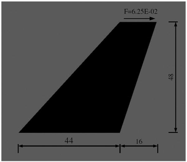
Set up for Cook's membrane problem.

The tip deflection as a function of the number of elements is shown in Fig. 3. The upper curve represents the computations with stabilization and the lower curve without stabilization. Mesh locking is observed for the mixed method without stabilization when a small number of elements is used whereas the stabilized version does not lock. When the mesh is refined, both curves converge to the same value.

Fig. 3.

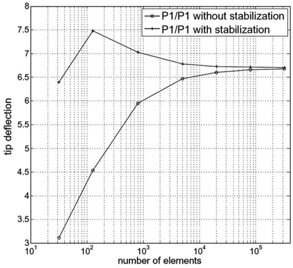
Tip deflection versus number of elements, with and without stabilization.

For the Galerkin formulation refining the mesh appears to solve the problem of mesh locking, but it does not stabilize the pressure mode. This can be seen in Fig. 4(a) and (b), where we have plotted the pressure distribution for the case with 5000 elements for the mixed method and the stabilized mixed method, respectively. For the plain mixed method we observe that the pressure fluctuates between about −25 to above +30, and the distribution is physically unrealistic. We note that these pressure values will also contaminate the stresses evaluated using this method. For the stabilized formulation we have a smooth and realistic pressure distribution, varying between −0.105 and 0.22. The pressure concentration seen at the right bottom corner is to be expected due to the bending of this structure under the action of the prescribed force.

Fig. 4.

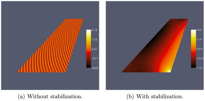
Pressure distribution with 5000 elements.

4.2. Solution of the Inverse problem

In this section we evaluate the performance of our inverse problem solution strategy on synthetic data. We begin with a “known” material property distribution. We load this specimen by solving the forward problem and record the displacement fields. Thereafter we add noise to the displacement fields to generate the “measured” displacements and use these in our algorithm to reconstruct the spatial distribution of the material properties. The mesh to compute the synthetic data is the same as for solving the inverse problem. However, we do not commit an inverse crime, as we are adding noise to our displacement field before we reconstruct the material properties. We compare these reconstructions with the original distributions in order to assess the performance of our approach. In our initial tests we find that our approach yields good reconstructions of the shear modulus but poor reconstructions of the nonlinear parameter. We propose and test approaches to improve these reconstructions in Sections 4.3 and 4.5.

4.2.1. Creating synthetic data

The material property distributions for our synthetic specimen are given in Fig. 5(a) and (b). For the shear modulus we have two inclusions in a homogeneous background. Both inclusions have the same shear modulus value of 5 and the shear modulus in the background is unity. For the nonlinear parameter there are three inclusions with values of 5, 15 and 10 embedded in a homogeneous background with a value of unity. The measured field is created by solving the forward problem and then adding white Gaussian noise to be consistent with noisy experimental data. We use 7200 linear triangular elements on a unit square to solve the forward problem. We consider two loading scenarios. In the first instance we compress the specimen in the vertical direction by prescribing a uniform displacement in the positive Y direction to the bottom edge and keeping the top edge fixed in the Y direction. Both these edges are free to deform in the horizontal direction, and the lateral edges are completely traction free. We prescribe displacements of 2.0 × 10⁻³ and 0.2 units, corresponding to overall strains of 0.2% and 20% respectively, in order to generate a small deformation and a large deformation displacement field. In the second instance we rotate the loading state by 90° in the counter-clockwise direction. As a result we prescribe a uniform displacement in the horizontal direction along the right edge while holding the left edge fixed in the same direction. The top and bottom edges are left traction free, and overall strains of 0.2% and 20% are applied.

Fig. 5.

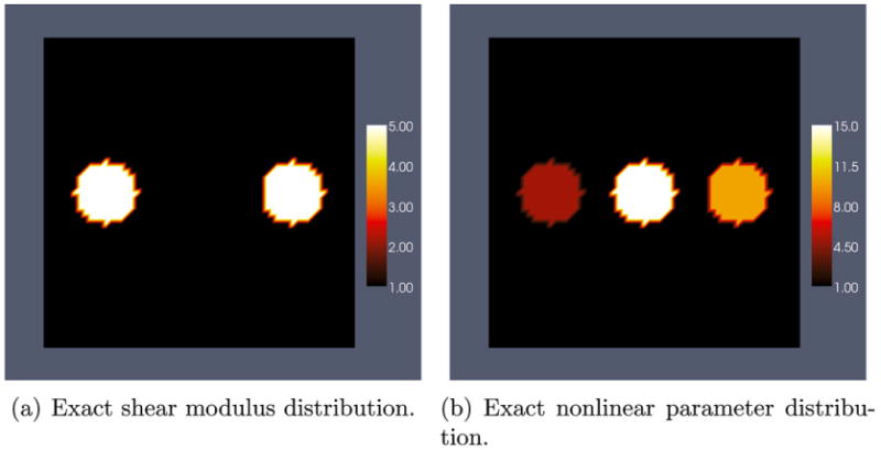
Exact material property distributions.

We have a total of four displacement fields that are used in the minimization process. We add to these displacement fields about 0.3%, 1% and 3% noise which corresponds to noise in strain of about 7.5%, 25.3%, and 74%, respectively. The noise is measured using the L₂ norm, and is given by

$$\frac{{\Vert \eta -{\eta }_{\mathit{\text{noise}}}\Vert }_0}{{\Vert \eta \Vert }_0},$$ (38)

where η can be thought of as a displacement or strain field without noise, and η_noise is the corresponding noisy field.

4.3. Simultaneous reconstructions

Using the four displacement fields with 1% noise we apply our method for reconstructing the shear modulus and the nonlinear parameter. The regularization parameter for μ and γ are chosen to be 1.0 × 10⁻⁷ and 1.0 × 10⁻⁸, respectively, corresponding to a Morozov parameter of 0.72, which is close to unity. We note that the Morozov discrepancy principle states that the value of the regularization parameter should be chosen such that the difference between the predicted and the noisy measured displacement field should be the same order as the difference between the clean and the noisy measured displacement. Thus the Morozov parameter is defined as

$$C=\frac{{\Vert \overline{\eta }-{\eta }_{\mathit{\text{noise}}}\Vert }_0}{{\Vert \eta -{\eta }_{\mathit{\text{noise}}}\Vert }_0}\approx 1.$$ (39)

In the equation above η̄ is the predicted displacement field.

In Fig. 6(b) we have plotted the reconstructed shear modulus next to the exact distribution Fig. 6(a). The shear modulus ratio of inclusion to background is very close to the exact value of 5. Fig. 7 shows the shear modulus value plotted along the horizontal line through the center of the inclusions. In Fig. 8(b) we have plotted the reconstruction of the nonlinear parameter next to the exact nonlinear parameter distribution. We observe that the nonlinear parameter is not well recovered. The comparison between the exact and reconstructed value of the nonlinear parameter along the horizontal centerline in Fig. 9 shows that the reconstructed value significantly underestimates the correct value. This was also observed in the compressible case in [12]. The reason for this is that the gradient of the objective function with respect to gamma is much smaller than the gradient with respect to μ for both the small and large deformation cases. That is $\frac{\partial \pi }{\partial \mu }\gg \frac{\partial \pi }{\partial \gamma }$. As a result the BFGS method, which utilizes these gradients, tends to alter the value of μ while leaving γ relatively unchanged at the initial guess of unity.

Fig. 6.

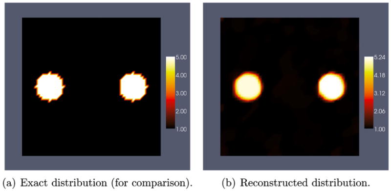
Shear modulus reconstruction using 4 displacement fields with 1% noise.

Fig. 7.

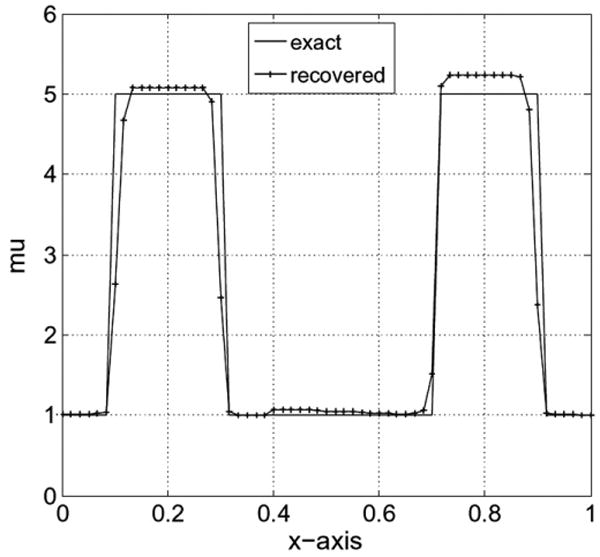
Shear modulus reconstruction using 4 displacement fields with 1% noise along the horizontal centerline.

Fig. 8.

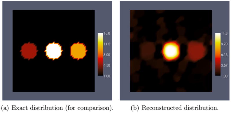
Nonlinear parameter reconstruction using 4 displacement fields with 1% noise.

Fig. 9.

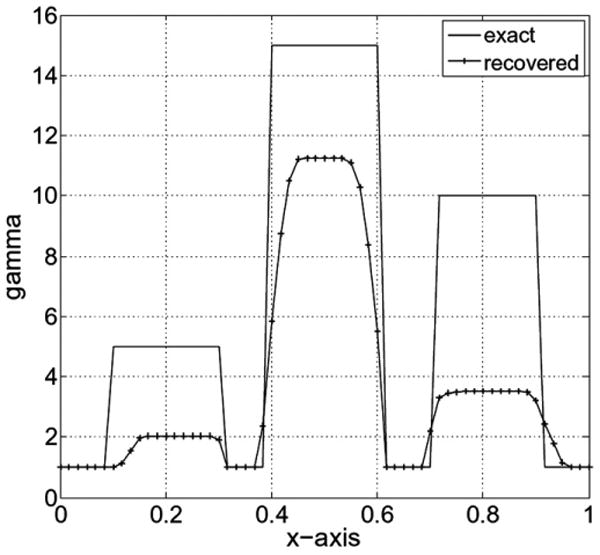
Nonlinear parameter reconstruction using 4 displacement fields with 1% noise along the horizontal centerline.

An explicit expression for the ratio $\frac{\partial \pi }{\partial \mu }/\frac{\partial \pi }{\partial \gamma }$ can be derived for a simple uniaxial tension/compression for a homogeneous material as given in Eq. (40).

$$\frac{\partial \pi }{\partial \mu }/\frac{\partial \pi }{\partial \gamma }=\frac{1}{\mu ({\lambda }^2+\frac{2}{\lambda }-3)}.$$ (40)

From (40) one can see that the ratio is only a function of the stretch and the shear modulus. The smaller the stretch is, the bigger becomes the ratio of the gradients. Considering a stretch of λ = 0.8 which corresponds to our total strain of 20% and a shear modulus of 1 results in a gradient ratio of around 7.

A simple fix to this problem is to re-scale the parameters μ and γ such that the value of the gradient is comparable in the large deformation case. In the small deformation case we still expect the gradient with respect to γ to be small as this data carries very little information about the nonlinear behavior of the material. This rescaling may be thought of as a diagonal preconditioning of the original system of equations. This idea is explored in the following section.

4.4. Simultaneous reconstructions with scaling

We replace the nonlinear parameter γ by ξγ in the formulation, so that the appropriate gradient changes from $\frac{\partial \pi }{\partial \gamma }$ to $\xi \frac{\partial \pi }{\partial \overline{\gamma }}$. Here ξ is the scaling factor which is chosen a priori such that $\frac{\partial \pi }{\partial \mu }\simeq \frac{\partial \pi }{\partial \gamma }$ in the large deformation case. For our example the appropriate value is ξ = 5.

Using the scaled version of γ in our formulation we reconstruct the material properties for the problem described in the previous section. We consider all three levels of noise. The regularization parameters for μ and γ as well as the corresponding Morozov parameters for all computations are listed in Table 1. We observe that the Morozov parameter is close to unity.

Table 1.

Parameters for material property reconstructions.

Noise in displacement (%)	Regularization parameter for μ	Regularization parameter for γ	Morozov parameter
0.3	1.5E–07	1.8E–09	0.69
1.0	5.0E–07	1.0E–08	0.71
3.0	2.0E–06	4.0E–08	0.70

For 1% noise the shear modulus and nonlinear parameter reconstructions are plotted in Fig. 10(b) and Fig. 12(b). We observe that both reconstructions are in good agreement with the exact distributions. In order to illustrate the effect of scaling γ, in Figs. 11 and 13 are plotted the shear modulus and the nonlinear parameter values along the horizontal centerline for the case with and without scaling. We observe that the scaled version recovers the exact contrast in γ much more accurately without losing contrast in the value of μ.

Fig. 10.

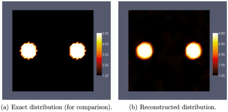
Shear modulus reconstruction using 4 displacement fields with 1% noise and scaling γ.

Fig. 12.

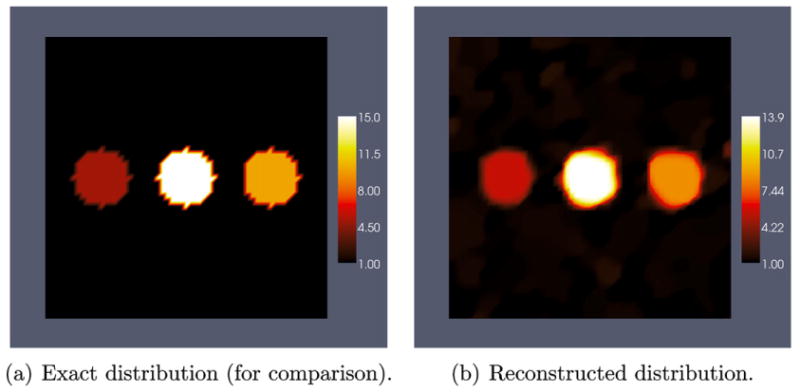
Nonlinear parameter reconstruction using 4 displacement fields with 1% noise and scaling γ.

Fig. 11.

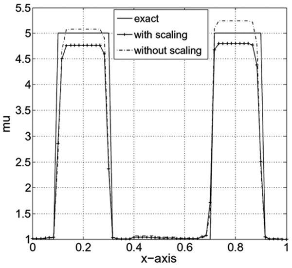
Shear modulus reconstruction along the horizontal centerline, using 4 displacement fields with 1% noise.

Fig. 13.

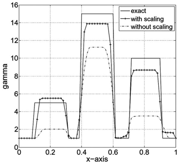
Nonlinear parameter along the horizontal centerline using 4 displacement fields with 1% noise and scaling γ.

Fig. 14(b) and (d) show reconstructions of the shear modulus using the scaled version of γ with 0.3% and 3% noise in the displacement, respectively. The reconstruction with 1.0% noise is also included in the figures for completeness. The corresponding horizontal centerline plot appears in Fig. 15. The reconstructions for the nonlinear parameter γ are shown in Fig. 16(b) and (d), and the corresponding horizontal centerline plots appear in Fig. 17.

Fig. 14.

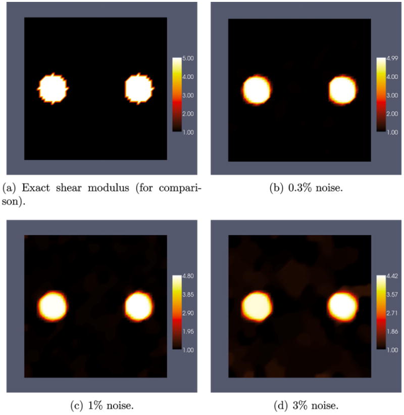
Shear modulus reconstruction after scaling γ for different noise levels.

Fig. 15.

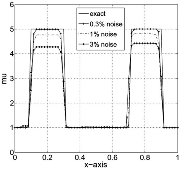
Shear modulus along the horizontal centerline after scaling γ for different noise levels.

Fig. 16.

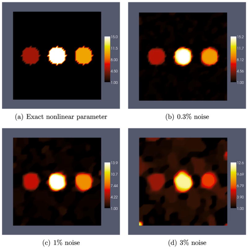
Nonlinear parameter reconstruction after scaling γ for different noise levels.

Fig. 17.

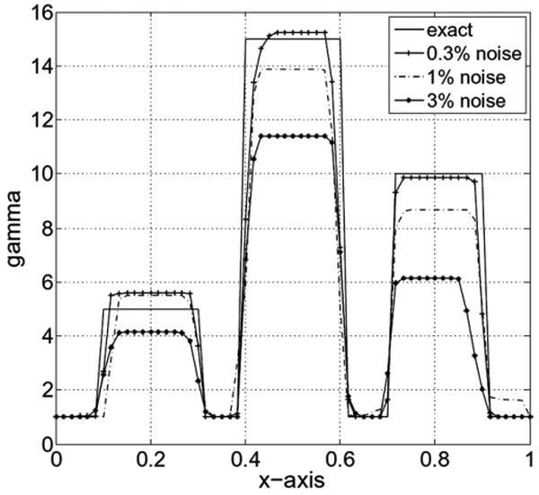
Nonlinear parameter along the horizontal centerline after scaling γ for different noise levels.

We note that even with a high noise level of 3% noise in the displacement, which corresponds here to a very high level of strain noise of 74%, we are able to distinguish the inclusions with respect to their stiffness and nonlinear behavior. The contrast improves dramatically with decreasing noise and regularization parameter, due to the reduction in the effect of TV regularization.

4.5. Sequential reconstructions

In the previous sections we have demonstrated the utility of rescaling the nonlinear parameter when the shear modulus and the nonlinear parameter are reconstructed simultaneously using small and large displacement fields. The need for rescaling can be avoided with the strategy of sequential optimization. This idea is based on the fact that small strain deformations are completely independent of the γ distribution. Thus, in the first step the two small displacement fields are used to reconstruct the shear modulus while the nonlinear parameter is held fixed at a small value. The regularization parameters and corresponding Morozov parameters are given in Table 2 for the different noise levels. The shear modulus reconstructions are plotted in Fig. 18(b) to (d) for the different noise levels. The corresponding plot through the horizontal centerline is presented in Fig. 19. We observe that the shear modulus reconstructions are very accurate and compare favorably with the simultaneous reconstructions.

Table 2.

Parameters for sequential reconstructions (for μ).

Noise in displacement (%)	Regularization parameter	Morozov parameter
0.3	1.5E–12	0.68
1.0	5.0E–12	0.68
3.0	2.0E–11	0.69

Fig. 18.

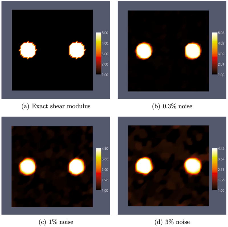
Sequential reconstruction of shear modulus. μ reconstructed from two small strain displacement fields, with different levels of noise. During μ reconstruction, γ is held fixed.

Fig. 19.

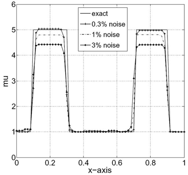
Sequential shear modulus reconstruction along the horizontal centerline.

In the next step we fix the previously computed shear modulus distributions and minimize the objective function with respect to γ using the two large displacement fields. The regularization parameter and the Morozov parameter are given in Table 3. The reconstructions for γ are presented in Fig. 20(b) to (d), while the values along the horizontal centerline appear in Fig. 21. We observe that the sequential approach performs as well as, if not better than, the scaled simultaneous approach.

Table 3.

Parameters for sequential reconstructions (for γ).

Noise in displacement (%)	Regularization parameter	Morozov parameter
0.3	1.8E–09	0.69
1.0	1.0E–08	0.71
3.0	4.0E–08	0.70

Fig. 20.

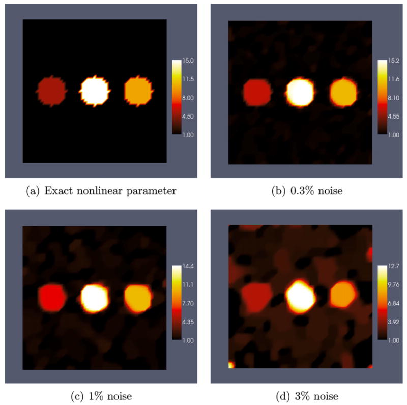
Sequential reconstruction of nonlinear parameter. γ is reconstructed from two large displacement fields, with different levels of noise added. During the reconstruction of γ, μ is held fixed to those distributions depicted in Fig. 18(b)–(d).

Fig. 21.

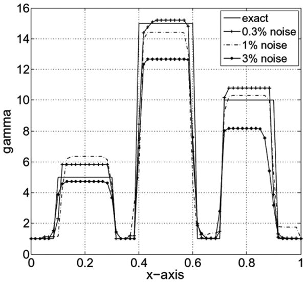
Nonlinear parameter reconstruction along the horizontal centerline.

5. Conclusions

In this paper we have developed and tested an approach for solving the inverse nonlinear elasticity problem for an incompressible hyperelastic solid. This problem arises in elasticity imaging, or elastography, where the displacement field inside the tissue is measured at different values of overall strain and images of the material parameters are sought. We pose this problem as a minimization problem, where we assume an exponential dependence of stress on strain, and find the distribution of material parameters which yields the best match between predicted and measured displacement fields. The predicted displacement fields are constrained to satisfy the equations of equilibrium.

We solve this problem by using a quasi-Newton algorithm and implement several numerical techniques that make the solution possible. We evaluate the gradient vector efficiently by making use of the adjoint equations and a novel continuation strategy in material parameters. We solve the forward and adjoint problems for an incompressible solid by using a stabilized finite element formulation that avoids mesh locking and spurious pressure modes. We propose a new strain energy density function with an exponential stress response that yields a deviatoric stress tensor and simplifies the interpretation of pressure for an incompressible material. Finally, we propose and implement a diagonal preconditioning and a decoupling approach to improve the reconstruction of the nonlinear parameter. We test and demonstrate the utility of these ideas as well as the performance of the overall approach on synthetically generated, noisy displacement data. Their application to experimentally measured displacement data will be considered in the near future.

Appendix A. Linearization of the stabilized weak form

In solving the forward problem as well as in solving the adjoint problem the linearization of the left hand side of the weak form about a given displacement and pressure field is required. Mathematically this is denoted by:

$$ℬ(\mathit{\text{W}},\Delta \mathit{\text{U}};\mathit{\text{β}},\mathit{\text{U}})=\underset{\varepsilon \to 0}{lim}\frac{d}{d\varepsilon }(\mathcal{A}(\mathit{\text{W}},\mathit{\text{U}}+\varepsilon \Delta \mathit{\text{U}};\mathit{\text{β}})+ℛ(\mathit{\text{W}},\mathit{\text{U}}+\varepsilon \Delta \mathit{\text{U}};\mathit{\text{β}})),$$ (A.1)

where ΔU ≡ [Δu, Δp]. The first term on the right hand side of (A.1) is given by

$$\underset{\varepsilon \to 0}{lim}\frac{d}{d\varepsilon }\mathcal{A}(\mathit{\text{W}},\mathit{\text{U}}+\varepsilon \Delta \mathit{\text{U}};\mathit{\text{β}})={\int }_{{\Omega }_0}{w}_{m,\alpha }({\delta }_{mn}{S}_{\alpha \beta }+F_{m\gamma }{F}_{n\eta }{\mathcal{C}}_{\gamma \alpha \eta \beta })\Delta u_{n,\beta }d{\Omega }_0+{\int }_{{\Omega }_0}qJ{F}_{i\alpha }^{-T}\Delta u_{i,\alpha }d{\Omega }_0-{\int }_{{\Omega }_0}{w}_{i,\alpha }J{F}_{\alpha i}^{-1}\Delta pd{\Omega }_0.$$ (A.2)

The second term is derived from (16) and is given by

$$\underset{\varepsilon \to 0}{lim}\frac{d}{d\varepsilon }ℛ(\mathit{\text{W}},\mathit{\text{U}}+\varepsilon \Delta \mathit{\text{U}};\mathit{\text{β}})=\sum _{e=1}^{n_{el}}2{\int }_{{\Omega }_0^e}\tau \left(2q{,}_{\alpha }p{,}_{\beta }\frac{{\partial }^{2}J}{\partial C_{\alpha \beta }\partial C_{\gamma \eta }}{F}_{i\gamma }\Delta u_{i,\eta }+q{,}_{\alpha }\frac{\partial J}{\partial C_{\alpha \beta }}\Delta p{,}_{\beta }\right)d{\Omega }_0,$$ (A.3)

where

$$\frac{{\partial }^{2}J}{\partial C_{\alpha \beta }\partial C_{\gamma \eta }}=-\frac{1}{2}\left(C_{\alpha \gamma }^{-1}{C}_{\beta \eta }^{-1}+C_{\alpha \eta }^{-1}{C}_{\beta \gamma }\right).$$ (A.4)

References

- 1.Gao L, Parker KJ, Lerner RM, Levinson SF. Imaging of the elastic properties of tissue – A review. Ultrasound in Medicine and Biology. 1996;22:959–977. doi: 10.1016/s0301-5629(96)00120-2. [DOI] [PubMed] [Google Scholar]
- 2.Parker KJ, Gao L, Lerner RM, Levinson SF. Techniques for elastic imaging: a review. IEEE Engineering in Medicine and Biology Magazine. 1996;15:52–59. [Google Scholar]
- 3.Ophir J, Alam SK, Garra B, Kallel F, Konofagou E, Krouskop T, Varghese T. Elastography: ultrasonic estimation and imaging of the elastic properties of tissues. Proceedings of the Institution of Mechanical Engineers Part H-Journal of Engineering in Medicine. 1999;213:203–233. doi: 10.1243/0954411991534933. [DOI] [PubMed] [Google Scholar]
- 4.Greenleaf JF, Fatemi M, Insana M. Selected methods for imaging elastic properties of biological tissues. Annual Review of Biomedical Engineering. 2003;5:57–78. doi: 10.1146/annurev.bioeng.5.040202.121623. [DOI] [PubMed] [Google Scholar]
- 5.Parker KJ, Taylor LS, Gracewski S, Rubens DJ. A unified view of imaging the elastic properties of tissue. Journal of the Acoustical Society of America. 2005;117:2705–2712. doi: 10.1121/1.1880772. [DOI] [PubMed] [Google Scholar]
- 6.Wellman P, Howe RH, Dalton E, Kern KA. Technical Report. Harvard BioRobotics Laboratory, Division of Engineering and Applied Sciences; Harvard University: 1999. Breast Tissue Stiffness in Compression is Correlated to Histological Diagnosis. [Google Scholar]
- 7.Samani A, Plewes D. A method to measure the hyperelastic parameters of ex vivo breast tissue samples. Physics in Medicine and Biology. 2004;49:4395–4405. doi: 10.1088/0031-9155/49/18/014. [DOI] [PubMed] [Google Scholar]
- 8.Oberai AA, Gokhale NH, Goenezen S, Barbone PE, Hall TJ, Sommer AM, Jiang J. Linear and nonlinear elasticity imaging of soft tissue in vivo: demonstration of feasibility. Physics in Medicine and Biology. 2009;54:1191–1207. doi: 10.1088/0031-9155/54/5/006. [DOI] [PMC free article] [PubMed] [Google Scholar]
- 9.Paszek MJ, Zahir N, Johnson KR, Lakins JN, Rozenberg GI, Gefen A, Reinhart-King CA, Margulies SS, Dembo M, Boettiger D, Hammer DA, Weaver VM. Tensional homeostasis and the malignant phenotype. Cancer Cell. 2005;8:241–254. doi: 10.1016/j.ccr.2005.08.010. [DOI] [PubMed] [Google Scholar]
- 10.Falzon G, Pearson S, Murison R. Analysis of collagen fibre shape changes in breast cancer. Physics in Medicine and Biology. 2008;53:6641–6652. doi: 10.1088/0031-9155/53/23/001. [DOI] [PubMed] [Google Scholar]
- 11.O'Hagan JJ, Samani A. Measurement of the hyperelastic properties of 44 pathological ex vivo breast tissue samples. Physics in Medicine and Biology. 2009;54:2557–2569. doi: 10.1088/0031-9155/54/8/020. [DOI] [PubMed] [Google Scholar]
- 12.Gokhale NH, Barbone PE, Oberai AA. Solution of the nonlinear elasticity imaging inverse problem: the compressible case. Inverse Problems. 2008;24 doi: 10.1016/j.cma.2010.12.018. [DOI] [PMC free article] [PubMed] [Google Scholar]
- 13.Veronda DR, Westmann RA. Mechanical characterization of skin-finite deformations. Journal of Biomechanics. 1970;3:111–122. IN9, 123–124. doi: 10.1016/0021-9290(70)90055-2. [DOI] [PubMed] [Google Scholar]
- 14.Babuska I. The finite element method with Lagrangian multipliers. Numerische Mathematik. 1973;20:179–192. [Google Scholar]
- 15.Brezzi F. Existence, uniqueness and approximation of saddle-point problems arising from Lagrangian multipliers. Revue Francaise D Automatique Informatique Recherche Operationnelle. 1974;8:129–151. [Google Scholar]
- 16.Klaas O, Maniatty A, Shephard MS. A stabilized mixed finite element method for finite, elasticity.: formulation for linear displacement and pressure interpolation. Computer Methods in Applied Mechanics and Engineering. 1999;180:65–79. [Google Scholar]
- 17.Maniatty AM, Liu Y, Klaas O, Shephard MS. Higher order stabilized finite element method for hyperelastic finite deformation. Computer Methods in Applied Mechanics and Engineering. 2002;191:1491–1503. [Google Scholar]
- 18.Blatz PJ, Chu BM, Wayland H. On the mechanical behavior of elastic animal tissue. Journal of Rheology. 1969;13:83–102. [Google Scholar]
- 19.Hughes TJR. The Finite Element Method-linear Static and Dynamic Finite Element Analysis. Dover Publications; Mineola, New York, USA: 2000. [Google Scholar]
- 20.Simo JC, Hughes TJR. On the variational foundations of assumed strain methods. Journal of Applied Mechanics-Transactions of the ASME. 1986;53:51–54. [Google Scholar]
- 21.Hughes TJR, Franca LP, Balestra M. A new finite element formulation for computational fluid dynamics: V. circumventing the Babuska–Brezzi condition: a stable Petrov–Galerkin formulation of the stokes problem accommodating equal-order interpolations. Computer Methods in Applied Mechanics and Engineering. 1986;59:85–99. [Google Scholar]
- 22.Krouskop TA, Wheeler TM, Kallel F, Garra BS, Hall T. Elastic moduli of breast and prostate tissues under compression. Ultrasonic Imaging. 1998;20:260–274. doi: 10.1177/016173469802000403. [DOI] [PubMed] [Google Scholar]
- 23.Humphrey JD. Mechanics of the arterial wall: review and directions. Critical Reviews in Biomedical Engineering. 1995;23:1–162. [PubMed] [Google Scholar]
- 24.Byrd RH, Lu P, Nocedal J, Zhu CY. A limited memory algorithm for bound constrained optimization. SIAM Journal on Scientific Computing. 1995;16:1190–1208. [Google Scholar]
- 25.Vogel CR. Society for Industrial and Applied Mathematics. Philadelphia, PA, USA: 2002. Computational methods for inverse problems. [Google Scholar]
- 26.Oberai AA, Gokhale NH, Doyley MM, Bamber JC. Evaluation of the adjoint equation based algorithm for elasticity imaging. Physics in Medicine and Biology. 2004;49:2955–2974. doi: 10.1088/0031-9155/49/13/013. [DOI] [PubMed] [Google Scholar]
- 27.Natterer F, Wubbeling F. A propagation–backpropagation method for ultrasound tomography. Inverse Problems. 1995;11 [Google Scholar]
- 28.Dorn O, Bertete-Aguirre H, Berryman JG, Papanicolaou GC. A nonlinear inversion method for 3D electromagnetic imaging using adjoint fields. Inverse Problems. 1999;15 [Google Scholar]