Preparation and Analysis of Glycan Microarrays

INTRODUCTION

Investigations of carbohydrate-protein interactions have been revolutionized by the availability of glycan microarrays comprised of hundreds of defined glycan structures that can be interrogated with fluorescent-labeled carbohydrate-binding proteins or organisms. Researchers have spent years developing methods for determining the structures of complex glycans, and can now reap the benefits of that work by having access to structurally defined, chemo/enzymatically synthesized glycans in a format that addresses functional recognition of glycans. Historically, the specificities of many glycan-binding proteins (GBPs), which include lectins, receptors, and antibodies, have been defined by hapten inhibition of a binding or agglutination assay, where each individual test compound is added in a concentration-dependent manner. Such assays require labor-intensive, multi-point assays and often large amounts (micro- to milligram) of precious glycan reagents. The miniaturization of glycan-binding assays in a highly sensitive format using miniscule amounts of samples on glycan microarrays now permits the analysis of hundreds of test compounds simultaneously in a single assay. This minimizes the time and effort to obtain relatively quantitative information about glycan binding specificity using only nanograms of precious glycans.

The concept of assay miniaturization of solid phase assays as 100–200 micron “microspots” (Elkins, R.P. 1989) was successfully applied to detection of nucleic acids in the form of DNA chips or microarrays arrays in the late 1980’s (Kulesh, D.A., Clive, D.R., et al. 1987), as a multiplexing technique to study gene expression in a high throughput fashion (Heller, M.J. 2002, Pollack, J.R. 2009, Ramsay, G. 1998). This technology was extended to proteomic analysis by immobilization of a variety of captured molecules as microspots for binding of proteins (Kramer, S., Joos, T.O., Templin, M.F. 2005). Unlike DNA arrays, where the capture molecules are readily available due to the ability and simplicity of synthesizing DNA sequences, protein microarrays and glycan microarrays share a common problem in that the desired capture molecules are not readily available, and their production, especially for glycan targets, is time consuming and expensive.

Production of Glycan Microarrays

Due to the wide utilization of DNA and protein microarrays, there is available instrumentation in many institutional core facilities in the form of arraying robots or printers that can be used to produce glycan microarrays and scanners to monitor fluorescence signals from binding assays. In general, glycan microarray printing can be categorized into contact printing and non-contact printing. For contact printing, a set of steel pins (from 1 to 48) are dipped into solutions of functionalized glycans contained in a multi-well source plate, and transferred to the glass slides by directly blotting the pin on the glass slide surface. The amount of solution delivered to the substrate will be a function of the time the pin is in contact with the surface. Depending on the pin type, the samples are pre-blotted on a practice surface to reach a consistent spot morphology before the microarray is printed. The amount of pre-blotting and contact time can be tuned so that ~0.5 nL per spot is printed rapidly and reproducibly.

Non-contact printing can be accomplished with a Piezo-electronic printer that controls the delivery of sample solution (~0.3 nL, with <5% intra-tip variation) from a glass capillary using controlled electric signals. This process can be finely tuned with different printing buffers for uniform delivery from each tip (<10% inter-tip variation) resulting in more precise printing relative to contact printing. Without contacting the substrate, the size and morphology of the printed spots are also relatively homogeneous, resulting in more precise readouts than can be obtained with contact printing. The accuracy of printing by either approach is especially important when quantitative or semi-quantitative studies are desired. The printing pattern can be controlled to produce large arrays of thousands of spots or multiple subarrays on a single glass slide, which permits multiple analyses on a single slide. A very useful feature of the Piezo-electronic printing method is that the sample solution aspirated from the source place is recycled back to the source plate after printing, which is extremely important when only small amounts of rare samples are being printed. The major disadvantage of Piezo-electronic printers, however, is that the number of printing tips is limited to 4 or 8 due to their expense and complexity. Thus, it may require hours to print several slides, requiring special attention to the stability of the substrate, moisture, sample evaporation, and temperature, which are controlled by most instruments. The non-contact inkjet printer, which solved these problems, is well suited for high-throughput and accurate microarray printing, but it requires larger sample volumes.

The Solid Phase

Glycans are immobilized to produce microarrays on glass microscope slides where the glycans are retained by either non-covalent interactions or covalent coupling. Nitrocellulose coated glass slides are currently the most common solid surface for non-covalent attachment, and the immobilization mechanism of nitrocellulose is presumably based on the hydrophobic interaction of the arrayed molecules with the membrane. Thus, glycans must be suitably derivatized with a hydrophobic component, as in neo-glycolipids (Feizi, T., Fazio, F., et al. 2003, Feizi, T., Stoll, M.S., et al. 1994, Liu, Y., Feizi, T., et al. 2007), before they can be efficiently printed and immobilized. Compared to normal glass slides, the nitrocellulose membrane layer provides a 3-dimensional presentation of the probes and a more even morphology among spots. However, the strong auto-fluorescence of the membrane at the same wavelength, as is used to detect the commonly used green fluorescent labels (FITC and Alexa488), limits the fluorescence detection to higher wavelength. Nitrocellulose coated glass slides are commercially available from several vendors, and can be used for printing glycolipids and neoglycolipids, glycoproteins, polysaccharides and other large molecules; however, they have limited use for defined low-molecular weight glycans attached to small linkers which are not hydrophobic enough to be efficiently adsorbed to the substrate.

Covalent immobilization provides more specific attachment of glycan probes via known functional groups. Over the last decade, the immobilization of glycans on glass slides has received extensive study and in most cases involved the manufacture of glass slides with chemically activated surfaces that are available from a number of vendors. Although free, reducing glycans can be directly printed by oxime/hydrozone formation on hydrazide or aminooxy-derivatized glass slides (Park, S., Lee, M.R., et al. 2007, Park, S., Lee, M.R., et al. 2009), the resulting glycosidic linkage may be either acyclic or cyclic with α- and β-configurations. With the exception of the aldehyde function of a reducing sugar, most glycans lack a selectively reactive functional group and therefore cannot be directly immobilized onto commercially available surface-activated glass slides. The glycans, therefore, require chemical modification to achieve successful immobilization. Efficient conjugation reactions have been explored for this purpose and include the thiol-maleimide reaction (Park, S. and Shin, I. 2002, Ratner, D.M., Adams, E.W., et al. 2004) and the amino-NHS ester/epoxy reactions (Blixt, O., Head, S., et al. 2004, de Boer, A.R., Hokke, C.H., et al. 2007, Disney, M.D. and Seeberger, P.H. 2004, Song, X., Xia, B., et al. 2008, Song, X., Xia, B., et al. 2009). Many commercially available, surface-activated glass slides are now available, and the two most commonly used glass slides for covalent immobilization are the N-hydroxysuccinimide (NHS)-ester and epoxy slides, which are reactive to free amino groups. While NHS-ester is more selective to primary alkylamine, epoxy slides are more reactive than NHS-slides and can be used with secondary amine and aromatic amine. Glycan-2,6-diaminopyridine (DAP) conjugates (Song, X., Xia, B., et al. 2008) and glycan-2-aminobenzamide (2AB)/2-aminobenzoic acid (2AA) conjugates (de Boer, A.R., Hokke, C.H., et al. 2007) can be printed on epoxy slides for screening of GBPs. The less specific reactivity of epoxy derivatized slides and generation of secondary/tertiary amine amines, on the other hand, might be the reason for overall higher background on epoxy compared to NHS-activated slides where the product of the NHS-ester and a primary amine is a chemically-inert amide. Glycoproteins and neo-glycoproteins can also be readily printed on these NHS- and epoxy slides (Luyai, A., Lasanajak, Y., et al. 2009, Oyelaran, O., Li, Q., et al. 2009). The surface of NHS- or epoxy slides can also be modified using bifunctional molecules with an amino group, such as for the application of click-chemistry (Krishnamurthy, V.R., Wilson, J.T., et al. 2010), which provides another bio-orthogonal approach to conjugate suitably derivatized glycans onto glass slides. Under normal conditions of storage in a desiccated environment at room temperature, the printed glycan microarrays are stable for years.

Applications of Glycan Microarrays for Functional Glycomics

Glycan microarrays are prepared by spotting extremely small amounts of individual glycans (50–100 femtomole), which are interrogated with suspected or known GBPs. The basic principle of the analysis is that each glycan is printed in discrete microspots (100–200 microns in diameter) in replicates on the glass microarray slide. After the slide is blocked and stabilized, the resulting array can be interrogated by addition of the GBP being analyzed to determine its ability to bind different glycans. The bound GBP is detected by a fluorescent method, and the fluorescence is quantified in a fluorescence scanner. This unit will describe the two types of glycan microarrays, the defined glycan array available from the Consortium for Functional Glycomics (CFG) and natural glycan arrays, and several examples of GBPs used to probe glycan microarrays.

GLYCAN BINDING PROTEIN SPECIFICITIES (MOTIF DEFINITION), EPITOPE ANALYSIS OF ANTI-GLYCAN ANTIBODIES, AND SPECIFICITY OF HOST-PATHOGEN INTERACTIONS USING THE DEFINED GLYCAN MICROARRAY PRODUCED BY THE CONSORTIUM FOR FUNCTIONAL GLYCOMICS (CFG)

Defined glycan arrays are comprised of known structures obtained from chemical synthesis or chemo-enzymatic synthesis. These compounds are generally available in milligram to gram quantities, and a large library of these synthetic glycans with amino-linkers installed at the reducing ends has been accumulated by the CFG with the support of National Institute of General Medical Sciences (NIGMS) to maintain the CFG glycan microarray (Blixt, O., Head, S., et al. 2004). The Glycan Array Synthesis Core (Core D) of the CFG prints these glycans on NHS-activated glass slides, and the resulting glycan microarrays have been used by the Protein-Glycan Interaction Core (Core H) of the CFG since November 2005 to carry out binding assays on the array as a service to investigators whose requests are approved by a Steering Committee. The CFG printed glycan array has grown since 2005 to contain over 511 glycan targets. The binding assays generate data that are used for determining GBP specificities or glycan-binding motifs, epitope analysis of anti-glycan antibodies, and specificity of pathogen binding to host cells. Knowledge of the specificity of a GBP contributes to understanding its function, which is consistent with the purpose of the CFG, which was formed to define the paradigms by which protein-carbohydrate interactions mediate cell communication.

The CFG glycan microarray is generated by printing the chemo/enzymatically synthesized glycans that have a primary amino group at their reducing end onto NHS-activated glass slides as described (Blixt, O., Head, S., et al. 2004). Briefly, the amine-containing glycans are diluted to 100 μM in print buffer (300 mM phosphate, pH 8.5 containing 0.005% Tween-20). The printing protocol is constructed so that 6 replicates of each glycan solution (~0.6 nL) are delivered to the slide surface. Covalent coupling of the glycans occurs in an atmosphere of 80% humidity for 30 minutes, and the slide is then placed in a desiccator overnight. The unreacted NHS groups are blocked with 50 mM ethanolamine in 50 mM borate buffer, pH 9.2 for 1 hour. The slides are rinsed with water, dried, and stored at room temperature in a desiccator until use. The list of glycans and the linker structures that are used to link the glycans to the slides for the various versions of the CFG glycan array can be found at: http://www.functionalglycomics.org/static/consortium/resources/resourcecoreh8.shtml. The synthetic glycan structures generally represent the terminal sequences found on N-glycans, O-glycans, and glycosphingolipids of mammalian tissues that are appropriate for screening the possible interactions with animal cell lectins and other GBPs.

Virtually any sample that is suspected of being a GBP can be screened on the glycan array providing fluorescent detection is available with any of the common fluorescent detection systems. Knowledge of the sample characteristics is critical to ensuring that the sample is active and can be detected using the chosen system. This usually requires additional assays, both before screening on the array to confirm sample activity, and after screening to validate any glycan binding that is detected.

BASIC PROTOCOL: The Binding Specificity of Biotinylated Plant Lectins Detected with Fluorescent Streptavidin

Lectins, or more generally glycan-binding proteins, are proteins that specifically bind to different carbohydrate structures via their defined carbohydrate-recognition domains (CRD) and do not catalyze a change in glycan structure. Their binding can range from low affinity interactions to high affinity and high avidity recognition through multiple CRDs (multivalency). Lectins, first identified in plants, have been identified in many microbes and animal species (Varki, A., Cummings, R.D., et al. 2009). Concanavalin A (ConA), one of the most widely used plant lectins, was the first to be crystallized in 1972 (Hardman, K.D. and Ainsworth, C.F. 1972). It is known to bind weakly to α-mannose and α-glucose, and with higher affinity to glycans containing one or more such residues. Its specificity was determined by a number of different assays involving the hapten inhibition of Con A in a variety of assays. The determination of the fine specificity of a lectin on the glycan microarray is accomplished by the simultaneous analysis of hundreds of glycans in a single experiment that would be much too labor intensive to attempt by hapten inhibition analyses. If a biotinylated lectin is used, it must be detected with fluorescent streptavidin, which is commercially available. Biotinylation of lectins can be easily accomplished using NHS-activated biotin, which reacts efficiently with primary amine groups to form stable amide bonds. Many biotinylation kits using NHS chemistries are also commercially available. Here we discuss the general method of assaying biotinylated lectins such as ConA on the CFG glycan microarray, and how data generated from these assays is processed and interpreted.

Materials

• Biotinylated lectin (commercially available, ex. Vector Labs)

• Alexa Fluor-488-Streptavidin (Invitrogen)

• Glycan printed slides, printed on one side of the slide

  DO NOT TOUCH THE PRINTED AREA

• Cover slips (Fisher Scientific, 12-545F)

• Humidified Slide processing chambers (Fisher Scientific, NC9091416), or homemade system using Petri Dish, with wet paper towels in the bottom of the chamber

• 100 ml Coplin jars for washing slides

• Tris-HCl (Fisher Scientific, BP152-1)

• NaCl (Fisher Scientific, S271-3)

• CaCl₂ (Fisher Scientific, C79-500)

• MgCl₂ (Fisher Scientific, BP214-500)

• Potassium Phosphate Monobasic (Fisher Scientific, P285-3)

• dH₂O

• BSA (Fisher Scientific, Bp1600-100)

• Tween-20 (EMD Biosciences, 655205)

• Sodium azide (Fisher Scientific, S227-500)

• ProScanArray Scanner (Perkin Elmer)

• ScanArray quantitation software (Scanarray Express, Perkin Elmer or Imagene, Biodiscovery)

Buffers

• TSM = 20mM Tris-HCl, pH 7.4 150mM NaCl, 2mM CaCl₂, 2mM MgCl₂

• TSM Wash Buffer (TSMWB) = TSM Buffer + 0.05% Tween-20

• TSM Binding Buffer (TSMBB) = TSM buffer + 0.05% Tween-20 + 1% BSA

Buffer Preparation

1L 10X TSM Washing Buffer Stock Solution

• 0.20M Tris-HCl

• 1.5M Sodium Chloride (NaCl)

• 0.02M Calcium Chloride (CaCl₂)

• 0.02M Magnesium Chloride (MgCl₂)

Weigh out required amount of Tris-HCl and NaCl. Dissolve in dH₂O and bring volume up to 800ml and pH solution and add HCL or NaOH to adjust pH to 7.4. Add appropriate concentrations of CaCl₂ and MgCl₂. Monitor pH while bringing up volume to 1000ml (1L) and adjust pH if necessary. Filter to increase shelf lifespan and store at Room Temperature (RT).

1X TSM

Add 10ml of 10X TSM buffer to 100ml of dH₂O

20% Tween-20

Add 20g of Tween-20 to 100ml of dH₂O

TSM Wash Buffer

• Add 10ml 10X TSM to 100ml of dH₂O

• Add 2.5ml of 20% Tween-20 for final concentration of 0.05%

TSM Binding Buffer

• For 100ml:

• 1X TSM buffer

• 2.5ml of 20% Tween-20

• 1g BSA

Protocol

1. Make working stocks of washing buffers (TSM, TSMWB, TSMBB, and H₂O) or collect reagents and bring to room temperature if they have been in the refrigerator.

2. Prepare 100 μl of sample by diluting biotinylated lectin in TSMBB to an appropriate final concentration required for the analysis. For lectins, a beginning concentration of 10 μg/ml should give ample binding. The protein solution can be further diluted to demonstrate its specificity.

3. Remove slide(s) from desiccator and label slide with sample name near barcode, outside of the markings used to delineate the position of the array on the slide.

4. Hydrate the slide by placing in a glass Coplin staining jar containing 100 ml of TSMWB for 5 minutes.

5. Remove excess liquid from slide by setting the slide upright to drain the liquid off.

6. Carefully apply 70 μl of sample (prepared in step 2) close to an edge of the slide within the markings used to delineate the position of the array on the slide.

7. Slowly lower cover slip onto the slide carefully to avoid trapping bubbles between the slide and the cover slip. Remove any bubbles trapped between the slide and cover slip by gently tapping with a pipette tip, if necessary, making sure the cover slip remains between the markings used to delineate the position of the array on the slide.

8. Incubate slide in a humidified tray in the dark for 1 hour at room temperature.

9. Remove cover slip by gently allowing it to slip off into the glass trash/biohazard trash.

10. Wash the slide by gently dipping 4 times (3 – 5 seconds each) into 100 ml of each of each of the following buffers in Coplin Jars: TSMWB, TSM

11. Remove excess TSM from slide by tipping the slide upright.

12. Add 70 μl of Streptavidin-AlexaFluor-488 at the appropriate amount (ex. 5 μg/ml) in TSMBB.

13. Apply cover slip as above (step 7) and incubate as above (step 8) in the dark.

14. After 1 hour incubation, remove cover slip by gently allowing it to slip off into the glass trash/biohazard trash.

15. Wash the slide by gently dipping 4 times into 100 ml of each of the following buffers in Coplin Jars: TSMWB, TSM, dH₂O

16. Spin slide in slide centrifuge for ~ 15 seconds or remove water under a gentle stream of nitrogen and air dry for 5 minutes.

17. Scan slide with a fluorescent scanner at the appropriate wavelengths

    For Alexa Fluor 488-labeled streptavidin, scan with 488 nm lamp. Save the image.

18. Process the slide with appropriate quantitation software.

Anticipated Results

An active lectin or GBP will produce detectable binding to the glycan microarray provided that a least one glycan recognized by the GBP is on the microarray. Common reasons for an inconclusive result on the glycan array (weak or no binding) is that the GBP has lost activity prior to analysis due to inappropriate storage or shipping conditions, processing prior to analysis, or to biotinylation that may disrupt its binding site. Obviously, one must also consider that the CFG glycan array contains only a subset of the possible glycans; therefore, an active lectin could generate a negative result because its glycan ligand(s) are not present on the array.

The data generated from the glycan microarray screening is an image of fluorescence bound to each spot. This image is the opened in an imaging and quantification program so that the intensity of fluorescence at each spot can be measured. Once the image is opened, a grid file is placed over the image and aligned using reference spots of biotin that are visualized with the fluorescent streptavidin detection reagent. This process allows the grid to be properly aligned over each data spot. The fluorescence corresponding to each spot is then quantified, processed, and tabulated. A macro program in Excel is then used to determine the average fluorescence of the 6 replicate spots. The macro processes the data further to remove the high and low value of the 6, leaving 4 values which are averaged and the standard deviation (STDEV), standard error of the mean (SEM) and coefficient of variation (STDEV ÷ Mean) expressed as a percentage (%CV) are determined for each glycan. The output from the analysis is a histogram and a table as shown in Figure 1 and Table 1. Figure 1 (top panel) shows a portion of the image from the fluorescence scanner and the pattern of replicate samples (n=6). The lower panel shows a computer-generated histogram of binding, where the average relative fluorescence units (RFU) for a sample of biotinylated ConA at a concentration of 1 μg/ml binding to each of 442 glycans on version 4.0 of the array. Table 1 displays the binding to glycans in order of highest relative fluorescence units (RFU) to lowest for the top 80 glycans. The complete list of glycans found on this version as well as all version of the CFG array can be found at: http://www.functionalglycomics.org/static/consortium/resources/resourcecoreh8.shtml.

Figure 1.

Con A binding to the CFG glycan array. The top panel is an image of fluorescently detected Con A binding to the glycan array slide. The replicates of one set of 6 spots, corresponding to one glycan, are noted. The bottom panel is a histogram of quantified Con A binding to the glycan array, where the x-axis is the chart number (glycan number) and the y-axis is relative fluorescent units (RFU).

Table 1.

Con A (1 μg/ml) binding to the CFG array v4.0. The table displays: the number in the ordered list (1–80), the chart number corresponding to the histogram (Figure 1), the glycan structure, the relative fluorescence units (RFU) of binding, the standard deviation (STDEV) of binding, and the percent coefficient of variance (%CV) of binding. The glycans are listed in order of highest binding RFU to lowest, up to 80 glycans. Structures of the linkers coupling the glycans to the NHS-derivatized glass surface of the array are indicated at the bottom.

#	Chart #	Structure	RFU	STDEV	% CV
1	47	Manα1-3(Manα1-6)Manβ1-4GlcNAcβ1-4GlcNAcβ-Sp12	60832	6406	11
2	52	Neu5Acα2-6Galβ1-4GlcNAcβ1-2Manα1-3(Neu5Acα2-6Galβ1-4GlcNAcβ1-2Manα1-6)Manβ1-4GlcNAcβ1-4GlcNAcβ-Sp8	54802	8809	16
3	392	Neu5Acα2-3Galβ1-3GlcNAcβ1-2Manα1-3(Neu5Acα2-3Galβ1-3GlcNAcβ1-2Manα1-6)Manβ1-4GlcNAcβ1-4GlcNAc-Sp19	48607	12931	27
4	348	Galβ1-4GlcNAcβ1-2Manα1-3(Galβ1-4GlcNAcβ1-2Manα1-6)Manβ1-4GlcNAcβ1-4(Fucα1-6)GlcNAcβ-Sp22	48582	16808	35
5	383	Galβ1-4GlcNAcβ1-2(Galβ1-4GlcNAcβ1-4)Manα1-3(Galβ1-4GlcNAcβ1-2(Galβ1-4GlcNAcβ1-6)Manα1-6)Manβ1-4GlcNAcβ1-4GlcNAcβ-Sp21	45986	10426	23
6	313	Neu5Acα2-3Galβ1-4GlcNAcβ1-2Manα1-3(Neu5Acα2-6Galβ1-4GlcNAcβ1-2Manα1-6)Manβ1-4GlcNAcβ1-4GlcNAcβ-Sp12	44754	14563	33
7	359	Galα1-3Galβ1-4GlcNAcβ1-2Manα1-3(Galα1-3Galβ1-4GlcNAcβ1-2Manα1-6)Manβ1-4GlcNAcβ1-4GlcNAcβ-Sp20	43621	8673	20
8	199	Manα1-2Manα1-3(Manα1-2Manα1-6)Manα-Sp9	43349	1667	4
9	51	Neu5Acα2-6Galβ1-4GlcNAcβ1-2Manα1-3(Neu5Acα2-6Galβ1-4GlcNAcβ1-2Manα1-6)Manβ1-4GlcNAcβ1-4GlcNAcβ-KVANKT*	43058	14556	34
10	399	Galα1-4Galβ1-3GlcNAcβ1-2Manα1-3(Galα1-4Galβ1-3GlcNAcβ1-2Manα1-6)Manβ1-4GlcNAcβ1-4GlcNAcβ-Sp19	42661	14809	35
11	198	Manα1-2Manα1-2Manα1-3Manα-Sp9	42422	8146	19
12	205	Manα1-3(Manα1-2Manα1-2Manα1-6)Manα-Sp9	41741	6952	17
13	347	GlcNAcβ1-2Manα1-3(GlcNAcβ1-2Manα1-6)Manβ1-4GlcNAcβ1-4(Fucα1-6)GlcNAcβ-Sp22	41416	7444	18
14	340	Manα1-3(Neu5Acα2-6Galβ1-4GlcNAcβ1-2Manα1-6)Manβ1-4GlcNAcβ1-4GlcNAc-Sp12	41257	15051	36
15	54	Neu5Acα2-6Galβ1-4GlcNAcβ1-2Manα1-3(Neu5Acα2-6Galβ1-4GlcNAcβ1-2Manα1-6)Manβ1-4GlcNAcβ1-4GlcNAcβ-Sp13	40848	8796	22
16	307	Manα1-6(Manα1-3)Manα1-6(Manα1-3)Manβ-Sp10	40807	3242	8
17	428	GlcNAcβ1-2Manα1-3(GlcNAcβ1-4)(GlcNAcβ1-2Manα1-6)Manβ1-4GlcNAcβ1-4GlcNAc-Sp21	40010	16499	41
18	350	Galβ1-3(Fucα1-4)GlcNAcβ1-2Manα1-3(Galβ1-3(Fucα1-4)GlcNAcβ1-2Manα1-6)Manβ1-4GlcNAcβ1-4GlcNAcβ-Sp19	39735	1479	4
19	400	Galα1-4Galβ1-4GlcNAcβ1-2Manα1-3(Galα1-4Galβ1-4GlcNAcβ1-2Manα1-6)Manβ1-4GlcNAcβ1-4GlcNAcβ-KVANKT*	39072	3115	8
20	349	Galβ1-3GlcNAcβ1-2Manα1-3(Galβ1-3GlcNAcβ1-2Manα1-6)Manβ1-4GlcNAcβ1-4(Fucα1-6)GlcNAcβ-Sp22	38876	6747	17
21	201	Manα1-6(Manα1-2Manα1-3)Manα1-6(Manα1-2Manα1-3)Manβ1-4GlcNAcβ1-4GlcNAcβ-Sp12	38344	2895	8
22	315	Neu5Acα2-6Galβ1-4GlcNAcβ1-2Manα1-3(GlcNAcβ1-2Manα1-6)Manβ1-4GlcNAcβ1-4GlcNAcβ-Sp12	37868	5911	16
23	314	Neu5Acα2-6Galβ1-4GlcNAcβ1-2Manα1-3(Galβ1-4GlcNAcβ1-2Manα1-6)Manβ1-4GlcNAcβ1-4GlcNAcβ-Sp12	37828	5194	14
24	48	Manα1-3(Manα1-6)Manβ1-4GlcNAcβ1-4GlcNAcβ-Sp13	37798	1296	3
25	200	Manα1-2Manα1-3Manα-Sp9	37736	933	2
26	202	Manα1-2Manα1-6(Manα1-3)Manα1-6(Manα1-2Manα1-2Manα1-3)Manβ1-4GlcNAcβ1-4GlcNAcβ-Sp12	37735	1065	3
27	53	Neu5Acα2-6Galβ1-4GlcNAcβ1-2Manα1-3(Neu5Acα2-6Galβ1-4GlcNAcβ1-2Manα1-6)Manβ1-4GlcNAcβ1-4GlcNAcβ-Sp12	37597	29001	77
28	309	Manα1-2Manα1-2Manα1-3(Manα1-2Manα1-6(Manα1-2Manα1-3)Manα1-6)Manα-Sp9	37072	2808	8
29	49	GlcNAcβ1-2Manα1-3(GlcNAcβ1-2Manα1-6)Manβ1-4GlcNAcβ1-4GlcNAcβ-Sp13	37069	5525	15
30	204	Manα1-3(Manα1-6)Manα-Sp9	37025	2052	6
31	321	Neu5Acα2-6Galβ1-4GlcNAcβ1-2Manα1-3(Neu5Acα2-3Galβ1-4GlcNAcβ1-2Manα1-6)Manβ1-4GlcNAcβ1-4GlcNAcβ-Sp12	36779	657	2
32	341	Neu5Acα2-6Galβ1-4GlcNAcβ1-2Manα1-3(Manα1-6)Manβ1-4GlcNAcβ1-4GlcNAc-Sp12	36607	6024	16
33	308	Manα1-2Manα1-2Manα1-3(Manα1-2Manα1-6(Manα1-3)Manα1-6)Manα-Sp9	36154	1155	3
34	346	Galβ1-4GlcNAcβ1-2Manα1-3(Manα1-6)Manβ1-4GlcNAcβ1-4GlcNAcβ-Sp12	35632	2840	8
35	203	Manα1-2Manα1-2Manα1-3(Manα1-2Manα1-3(Manα1-2Manα1-6)Manα1-6)Manβ1-4GlcNAcβ1-4GlcNAcβ-Sp12	35519	5161	15
36	207	Manα1-6(Manα1-3)Manα1-6(Manα1-3)Manβ1-4GlcNAcβ1-4 GlcNAcβ-Sp12	33294	2069	6
37	319	Galβ1-3GlcNAcβ1-2Manα1-3(Galβ1-3GlcNAcβ1-2Manα1-6)Manβ1-4GlcNAcβ1-4GlcNAcβ-Sp19	33245	1625	5
38	360	Manα1-3(Galβ1-4GlcNAcβ1-2Manα1-6)Manβ1-4GlcNAcβ1-4GlcNAcβ-Sp12	33065	1142	3
39	311	Neu5Acα2-3Galβ1-3(Neu5Acα2-6)GalNAcα-Sp14	32967	3614	11
40	424	Galα1-3(Fucα1-2)Galβ1-4GlcNAcβ1-2Manα1-3(Galα1-3(Fucα1-2)Galβ1-4GlcNAcβ1-2Manα1-6)Manβ1-4GlcNAcβ1-4(Fucα1-6)GlcNAcβ-Sp22	32937	5214	16
41	301	GlcNAcβ1-2Manα1-3(GlcNAcβ1-2Manα1-6)Manβ1-4GlcNAcβ1-4GlcNAcβ-Sp12	32746	3746	11
42	292	Galβ1-4GlcNAcβ1-2Manα1-3(Neu5Acα2-6Galβ1-4GlcNAcβ1-2Manα1-6)Manβ1-4GlcNAcβ1-4GlcNAcβ-Sp12	32571	2395	7
43	356	Fucα1-2Galβ1-3GlcNAcβ1-2Manα1-3(Fucα1-2Galβ1-3GlcNAcβ1-2Manα1-6)Manβ1-4GlcNAcβ1-4GlcNAcβ-Sp20	32132	7371	23
44	361	Galβ1-3(Fucα1-4)GlcNAcβ1-2Manα1-3(Galβ1-3(Fucα1-4)GlcNAcβ1-2Manα1-6)Manβ1-4GlcNAcβ1-4(Fucα1-6)GlcNAcβ-Sp22	31622	4716	15
45	50	Galβ1-4GlcNAcβ1-2Manα1-3(Galβ1-4GlcNAcβ1-2Manα1-6)Manβ1-4GlcNAcβ1-4GlcNAcβ-Sp12	30274	4211	14
46	206	Manα1-6(Manα1-3)Manα1-6(Manα1-2Manα1-3)Manβ1-4GlcNAcβ1-4GlcNAcβ-Sp12	30126	413	1
47	391	Galα1-3Galβ1-3(Fucα1-4)GlcNAcβ1-2Manα1-3(Galα1-3Galβ1-3(Fucα1-4)GlcNAcβ1-2Manα1-6)Manβ1-4GlcNAcβ1-4GlcNAc-Sp19	30024	5486	18
48	393	Galβ1-4GlcNAcβ1-2Manα1-3(GlcNAcβ1-2Manα1-6)Manβ1-4GlcNAcβ1-4GlcNAc-Sp12	30019	1285	4
49	300	GlcNAcβ1-2Manα1-3(Neu5Acα2-6Galβ1-4GlcNAcβ1-2Manα1-6)Manβ1-4GlcNAcβ1-4GlcNAcβ-Sp12	29826	2580	9
50	370	Galα1-3(Fucα1-2)Galβ1-3GlcNAcβ1-2Manα1-3(Galα1-3(Fucα1-2)Galβ1-3GlcNAcβ1-2Manα1-6)Manβ1-4GlcNAcβ1-4GlcNAcβ-Sp20	29685	4674	16
51	320	Neu5Acα2-3Galβ1-4GlcNAcβ1-2Manα1-3(Neu5Acα2-3Galβ1-4GlcNAcβ1-2Manα1-6)Manβ1-4GlcNAcβ1-4GlcNAcβ-Sp12	29652	1878	6
52	394	GlcNAcβ1-2Manα1-3(Galβ1-4GlcNAcβ1-2Manα1-6)Manβ1-4GlcNAcβ1-4GlcNAc-Sp12	28946	4066	14
53	390	Galα1-3Galβ1-3GlcNAcβ1-2Manα1-3(Galα1-3Galβ1-3GlcNAcβ1-2Manα1-6)Manβ1-4GlcNAcβ1-4GlcNAc-Sp19	28572	2585	9
54	357	Fucα1-2Galβ1-4GlcNAcβ1-2Manα1-3(Fucα1-2Galβ1-4GlcNAcβ1-2Manα1-6)Manβ1-4GlcNAcβ1-4GlcNAcβ-Sp20	27555	9860	36
55	423	Fucα1-2Galβ1-3GlcNAcβ1-2Manα1-3(Fucα1-2Galβ1-3GlcNAcβ1-2Manα1-6)Manβ1-4GlcNAcβ1-4(Fucα1-6)GlcNAcβ-Sp22	27552	4784	17
56	337	GlcNAcα1-4Galβ1-4GlcNAcβ1-3Galβ1-4(Fucα1-3)GlcNAcβ1-3Galβ1-4(Fucα1-3)GlcNAcβ-Sp0	25962	2212	9
57	384	GlcNAcβ1-2(GlcNAcβ1-4)Manα1-3(GlcNAcβ1-2Manα1-6)Manβ1-4GlcNAcβ1-4GlcNAc-Sp21	25026	3472	14
58	368	Galα1-3Galβ1-4(Fucα1-3)GlcNAcβ1-2Manα1-3(Galα1-3Galβ1-4(Fucα1-3)GlcNAcβ1-2Manα1-6)Manβ1-4GlcNAcβ1-4GlcNAcβ-Sp20	21683	850	4
59	425	Galβ1-3GlcNAcβ1-2Manα1-3(Galβ1-3GlcNAcβ1-2(Galβ1-3GlcNAcβ1-6)Manα1-6)Manβ1-4GlcNAcβ1-4GlcNAcβ-Sp19	21266	2040	10
60	430	GlcNAcβ1-2Manα1-3(GlcNAcβ1-4)(GlcNAcβ1-6(GlcNAcβ1-2)Manα1-6)Manβ1-4GlcNAcβ1-4GlcNAc-Sp21	20772	2138	10
61	322	Galβ1-4(Fucα1-3)GlcNAcβ1-2Manα1-3(Galβ1-4(Fucα1-3)GlcNAcβ1-2Manα1-6)Manβ1-4GlcNAcβ1-4GlcNAcβ-Sp20	19979	713	4
62	367	Galα1-3(Fucα1-2)Galβ1-4GlcNAcβ1-2Manα1-3(Galα1-3(Fucα1-2)Galβ1-4GlcNAcβ1-2Manα1-6)Manβ1-4GlcNAcβ1-4GlcNAcβ-Sp20	18685	1782	10
63	369	GalNAcα1-3(Fucα1-2)Galβ1-3GlcNAcβ1-2Manα1-3(GalNAcα1-3(Fucα1-2)Galβ1-3GlcNAcβ1-2Manα1-6)Manβ1-4GlcNAcβ1-4GlcNAcβ-Sp20	18675	4618	25
64	418	GlcNAcβ1-2Manα1-3(GlcNAcβ1-2(GlcNAcβ1-6)Manα1-6)Manβ1-4GlcNAcβ1-4GlcNAcβ-Sp19	15686	718	5
65	306	Manα1-6Manβ-Sp10	14940	1099	7
66	411	GalNAcα1-3(Fucα1-2)Galβ1-4GlcNAcβ1-3GalNAcα-Sp14	12991	1910	15
67	366	GalNAcα1-3(Fucα1-2)Galβ1-4GlcNAcβ1-2Manα1-3(GalNAcα1-3(Fucα1-2)Galβ1-4GlcNAcβ1-2Manα1-6)Manβ1-4GlcNAcβ1-4GlcNAcβ-Sp20	12858	1808	14
68	380	Fucα1-2Galβ1-3(Fucα1-4)GlcNAcβ1-3(Galβ1-4GlcNAcβ1-6)Galβ1-4Glc-Sp21	12473	714	6
69	365	Galβ1-4GlcNAcβ1-2(Galβ1-4GlcNAcβ1-4)Manα1-3(Galβ1-4GlcNAcβ1-2Manα1-6)Manβ1-4GlcNAcβ1-4GlcNAc-Sp21	12174	529	4
70	432	Galβ1-4GlcNAcβ1-2Manα1-3(GlcNAcβ1-4)(Galβ1-4GlcNAcβ1-2)Manβ1-4GlcNAcβ1-4GlcNAc-Sp21	10944	1088	10
71	326	Neu5Acα2-3Galβ1-3(Fucα1-4)GlcNAcβ1-3Galβ1-3(Fucα1-4)GlcNAcβ-Sp0	10118	826	8
72	3	Manα-Sp8	9464	4147	44
73	375	(GalNAcβ1-4GlcNAcβ1-2Manα1-6)GalNAcβ1-4GlcNAcβ1-2Manα1-3Manβ1-4GlcNAcβ1-4GlcNAc-Sp12	9202	640	7
74	371	Fucα1-2Galβ1-3(Fucα1-4)GlcNAcβ1-2Manα1-3(Fucα1-2Galβ1-3(Fucα1-4)GlcNAcβ1-2Manα1-6)Manβ1-4GlcNAcβ1-4GlcNAcβ-Sp19	7346	1036	14
75	230	Neu5Acα2-3Galβ1-3(Fucα1-4)GlcNAcβ1-3Galβ1-4(Fucα1-3)GlcNAcβ-Sp0	5541	426	8
76	259	Neu5Acα2-6Galβ1-4GlcNAcβ1-3Galβ1-4(Fucα1-3)GlcNAcβ1-3Galβ1-4(Fucα1-3)GlcNAcβ-Sp0	5232	322	6
77	441	Fucα1-2Galβ1-4GlcNAcβ1-2(Fucα1-2Galβ1-4GlcNAcβ1-4)Manα1-3(Fucα1-2Galβ1-4GlcNAcβ1-2Manα1-6)Manβ1-4GlcNAcβ1-4GlcNAcβ-Sp12	5028	1007	20
78	299	GlcAβ1-3GlcNAcβ-Sp8	4602	1026	22
79	373	Neu5Acα2-6Galβ1-4GlcNAcβ1-3GalNAc-Sp14	3711	1209	33
80	416	Galβ1-4(Fucα1-3)GlcNAcβ1-2Manα1-3(Galβ1-4(Fucα1-3)GlcNAcβ1-2Manα1-6)Manβ1-4GlcNAcβ1-4(Fucα1-6)GlcNAcβ-Sp22	3459	648	19
Chemical Linkers
Sp0		CH2CH2NH2
Sp8		CH2CH2CH2NH2
Sp9		CH2CH2CH2CH2CH2NH2
Sp10		NHCOCH2NH2
Sp12		Asparagine
Sp13		Glycine
Sp14		Threonine
Sp19		EN or NK
Sp20		GENR
Sp21		N(CH3)OCH2CH2NH2
Sp22		NST
*		KVANKT, where the glycan is linked to the Asparagine (N)

The data are then assessed with regard to: patterns or motifs of binding, structures that are not bound, level of fluorescence, and standard deviation or %CV. It is clear from this analysis that branched, high-mannose type glycans with multiple terminal α-linked mannose residues populate the list of structures that are bound the best by ConA. At higher concentrations of Con A (>100 μg/ml) this pattern is not observed since under these conditions, binding goes above the linear range of the scanner, which is between 0 and 50,000 RFU. Thus, to obtain interpretable data it is necessary to ensure that the assay results are within the linear range of the instrument. To obtain a more detailed picture of binding specificity, GBPs are assayed at multiple concentrations on the glycan array. As the GBP concentration is decreased, weaker binding glycans disappear from the histogram, thus a concentration-dependent analysis provides information on the relative binding strengths of the GBP for each glycan. A ranking of the ligands can performed at each GBP concentration with the following calculation: Rank = 100 × [RFU bound/highest RFU]. Comparing the glycan structures based on their ranking (strength of binding) can provide a more accurate picture of the binding specificity for a given GBP. The ranking data for ConA is shown in Table 2. A concentration analysis of ConA shows a ConA binding motif of terminal, branched α-linked mannose in the 2, 3, and 6 position on high mannose type N-glycan structures, which are highlighted in red in the table and have high rankings from 85 to 50. Substitutions to this motif, as is found in more complex type N-glycans by addition of N-acetylglucosamine, galactose, and sialic acid, decrease the glycan rankings to less than 50 indicating a second motif of ConA binding to biantennary N-glycans.

Table 2.

Ranking of Con A binding to the CFG array v4.0 at 1 μg/ml. The table displays: the glycan structure, the average relative fluorescence units (RFU) of binding, the percent binding compared to the maximum binding, and the average rank of each glycan over the 3 concentrations tested. Structures of the spacers are indicated at the end of Table 1. Red indicates the mannose residues present in the binding motif. Blue highlights the highest ranked glycan at each concentration and the glycan with the highest overall average ranking.

#	Glycan Structure	Con A 1 μg/ml		Con A 0.01 μg/ml		Con A 0.001 μg/ml		Avg. Rank
		Avg. RFU	% of MAX	Avg. RFU	% of MAX	Avg. RFU	% of MAX
1	Manα1-2Manα1-3(Manα1-2Manα1-6)Manα-Sp9	43349	71	23490	88	2857	96	85
2	Manα1-6(Manα1-3)Manα1-6(Manα1-2Manα1-3)Manβ1-4GlcNAcβ1-4GlcNAcβ-Sp12	30126	50	25552	96	2989	100	82
3	Manα1-2Manα1-2Manα1-3(Manα1-2Manα1-6(Manα1-2Manα1-3)Manα1-6)Manα-Sp9	37072	61	22295	84	2786	93	79
4	Manα1-3(Manα1-6)Manα-Sp9	37025	61	26599	100	2274	76	79
5	Manα1-2Manα1-6(Manα1-3)Manα1-6(Manα1-2Manα1-2Manα1-3)Manβ1-4GlcNAcβ1-4GlcNAcβ-Sp12	37735	62	23567	89	2245	75	75
6	Manα1-3(Manα1-2Manα1-2Manα1-6)Manα-Sp9	41741	69	24990	94	1836	61	75
7	Manα1-6(Manα1-2Manα1-3)Manα1-6(Manα1-2Manα1-3)Manβ1-4GlcNAcβ1-4GlcNAcβ-Sp12	38344	63	23313	88	1993	67	72
8	Manα1-2Manα1-2Manα1-3(Manα1-2Manα1-6(Manα1-3)Manα1-6)Manα-Sp9	36154	59	19646	74	2510	84	72
9	Manα1-6(Manα1-3)Manα1-6(Manα1-3)Manβ-Sp10	40807	67	20309	76	2105	70	71
10	Manα1-3(Manα1-6)Manβ1-4GlcNAcβ1-4GlcNAcβ-Sp12	60832	100	16941	64	1254	42	69
11	Manα1-6(Manα1-3)Manα1-6(Manα1-3)Manβ1-4GlcNAcβ1-4 GlcNAcβ-Sp12	33294	55	22076	83	1686	56	65
12	Manα1-3(Manα1-6)Manβ1-4GlcNAcβ1-4GlcNAcβ-Sp13	37798	62	20824	78	1600	54	65
13	Manα1-2Manα1-3Manα-Sp9	37736	62	16160	61	1639	55	59
14	Manα1-2Manα1-2Manα1-3Manα-Sp9	42422	70	13421	50	1247	42	54
15	Manα1-2Manα1-2Manα1-3(Manα1-2Manα1-3(Manα1-2Manα1-6)Manα1-6)Manβ1-4GlcNAcβ1-4GlcNAcβ-Sp12	35519	58	12290	46	1381	46	50
16	Neu5Acα2-6Galβ1-4GlcNAcβ1-2Manα1-3(Manα1-6)Manβ1-4GlcNAcβ1-4GlcNAc-Sp12	36607	60	11144	42	786	26	43
17	Galβ1-4GlcNAcβ1-2Manα1-3(Manα1-6)Manβ1-4GlcNAcβ1-4GlcNAcβ-Sp12	35632	59	10072	38	926	31	42
18	Manα1-3(Neu5Acα2-6Galβ1-4GlcNAcβ1-2Manα1-6)Manβ1-4GlcNAcβ1-4GlcNAcβ-Sp12	41257	68	7312	27	390	13	36
19	Manα1-3(Galβ1-4GlcNAcβ1-2Manα1-6)Manβ1-4GlcNAcβ1-4GlcNAcβ-Sp12	33065	54	7696	29	694	23	36
20	Neu5Acα2-6Galβ1-4GlcNAcβ1-2Manα1-3(Neu5Acα2-6Galβ1-4GlcNAcβ1-2Manα1-6)Manβ1-4GlcNAcβ1-4GlcNAcβ-Sp8	54802	90	1422	5	120	4	33
21	Galβ1-3GlcNAcβ1-2Manα1-3(Galβ1-3GlcNAcβ1-2Manα1-6)Manβ1-4GlcNAcβ1-4(Fucα1-6)GlcNAcβ-Sp22	38876	64	3576	13	639	21	33
22	Gala1-4Galβ1-3GlcNAcβ1-2Manα1-3(Galα1-4Galβ1-3GlcNAcβ1-2Manα1-6)Manβ1-4GlcNAcβ1-4GlcNAcβ-Sp19	42661	70	4832	18	258	9	32
23	GlcNAcβ1-2Manα1-3(GlcNAcβ1-2Manα1-6)Manβ1-4GlcNAcβ1-4GlcNAcβ-Sp13	37069	61	5961	22	384	13	32
24	Galβ1-4GlcNAcβ1-2Manα1-3(Galβ1-4GlcNAcβ1-2Manα1-6)Manβ1-4GlcNAcβ1-4(Fucα1-6)GlcNAcβ-Sp22	48582	80	2201	8	221	7	32
25	Galβ1-3GlcNAcβ1-2Manα1-3(Galβ1-3GlcNAcβ1-2Manα1-6)Manβ1-4GlcNAcβ1-4GlcNAcβ-Sp19	33245	55	5167	19	630	21	32

ALTERNATE PROTOCOL 1: The glycan epitopes for mouse monoclonal antibodies are detected using fluorescent anti-mouse IgG

Mouse monoclonal antibodies are often screened for their glycan binding specificity using the defined glycan microarray. This is accomplished by diluting the antibody to a suitable working concentration (1–50 μg/mL) and carrying out the assay as described above using a fluorescently labeled anti-mouse antibody against the correct immunoglobulin isotype (ex. IgG, IgM) for detection.

Materials

• Same materials as listed above for biotinylated lectins, except for the lectin

• Mouse monoclonal IgG antibody

• Cyanine 5- or Alexa Fluor 488-Streptavidin (ZYMED 43-4316 or Invitrogen)

• Appropriate secondary antibody to detect the monoclonal antibody being tested, fluorescently labeled if available (ex. Alexa Fluor-488 labeled anti-mouse IgG)

Buffers (see Basic Protocol for buffer preparation)

• TSM = 20mM Tris-HCl, pH 7.4 150mM NaCl, 2mM CaCl₂, 2mM MgCl₂

• TSM Wash Buffer (TSMWB) = TSM Buffer + 0.05% Tween-20

• TSM Binding Buffer (TSMBB) = TSM buffer + 0.05% Tween-20 + 1% BSA

Protocol

1. Make working stocks of washing buffers (TSM, TSMWB, TSMBB, and H₂O) or collect reagents and bring to room temperature if they have been in the refrigerator.

2. Prepare 100 μl of sample by diluting antibody in TSMBB or appropriate Binding Buffer based on properties of antibody to a final concentration of 1–50 ug/ml or an appropriate concentration required for the analysis.

3. Remove slide(s) from desiccator and label slide as necessary on the top of the slide.

   Do not write on the slide where the glycans are printed.

4. Hydrate the slide by placing in a glass Coplin staining jar containing 100 ml of TSMWB for 5 minutes.

5. Remove excess liquid from slide by setting the slide upright to drain the liquid off.

6. Carefully apply 70 μl of antibody (prepared in step 2) close to the left edge slide, being careful to cover the area of the slide where glycans are printed.

7. Slowly place cover slip on slide, trying to avoid the formation of bubbles in the sample under the cover slip.

   Remove any bubbles trapped between the slide and cover slip by gently tapping with a pipette tip, if necessary, making sure the cover slip remains between the markings used to delineate the position of the array on the slide.

8. Incubate slide in a humidified tray in the dark for 1 hour at room temperature.

9. Remove cover slip by gently allowing it to slip off into the glass waste/biohazard waste.

10. Wash the slide by gently dipping 4 times (3 – 5 seconds each) into 100 ml of each of each of the following buffers in Coplin Jars: TSMWB, TSM.

11. Remove excess water from slide by tipping the slide upright.

12. Add 70 μl of AlexaFluor-488-labeled (or other labeled) secondary antibody containing Cyanine 5-labeled streptavidin (final concentration 0.5 μg/ml) in TSMBB.

    Typically the streptavidin is used to align the printed spots on the array and is added to the dilution of antibody in the last step. Biotin is printed in the corners of each subarray for aligning the grid. A label that is different from the label on the detection reagent is usually used, so that the image of the biotin spots can be distinguished from the sample for alignment of the grid.

13. Apply the cover slip as above (step 7) and incubate as above (step 8).

14. After 1 hour incubation, remove cover slip by gently allowing it to slip off into the glass trash/biohazard trash.

15. Wash the slide by gently dipping 4 times into 100 ml of each of the following buffers in Coplin Jars: TSMWB, TSM, dH₂O.

16. Spin slide in slide centrifuge for ~ 15 seconds or remove water under a gentle stream of nitrogen.

17. Scan slide with a fluorescent scanner at the appropriate wavelengths For AlexaFluor488-labeled secondary antibodies, scan with 488 nm lamp, and to detect Cy5-streptavidin, scan with a 633 nm lamp. Save each image separately.

18. Process the slide with appropriate quantitation software.

Anticipated Results

The data output is the same as that described for a biotinylated GBP, and results can be used to define the glycan epitope of any type of antibody for which a secondary antibody is available. If an antibody is specific for a carbohydrate epitope, the repertoire of glycans on the CFG array should demonstrate some interaction with the antibody, to provide a minimal motif of binding. The detection of glycan epitopes can also be carried out on polyclonal antibodies or serum, but such analyses are more complex since most animal serum contains anti-immunoglobulin antibodies directed against glycans that have been encountered in the natural environment of the animal. For example, normal human serum contains IgGs that bind almost 50% of the glycans on the CFG glycan array (von Gunten, S., Smith, D.F., et al. 2009). Thus, epitope definition on monoclonal or affinity purified (on immobilized antigen) polyclonal antibodies is more conclusive than on serum. In addition, all detection reagents based on polyclonal antibodies or serum samples should be analyzed without the primary sample as a control.

ALTERNATE PROTOCOL 2: Specificity of Directly Labeled Influenza Virus Binding to Sialylated Glycans

Influenza A virus infects animal cells by initially binding to terminal α2-3- or α2-6-linked sialic acid residues of glycoconjugates, depending on whether the virus infects birds or mammals, respectively (Connor, R.J., Kawaoka, Y., et al. 1994, Rogers, G.N. and D’Souza, B.L. 1989). The availability of a large collection of sialyl-oligosaccharides on the CFG glycan array has permitted analyses of the involvement of the underlying glycan structures in this process by analyzing Influenza virus binding to the defined glycan array. Initial studies on Influenza A virus specificity were carried out using purified, recombinant hemagglutinin (Stevens, J., Blixt, O., et al. 2006), but many successful studies have been performed using fluorescent-labeled virus. Virus preparation can be labeled using commercially available succinimidyl esters of fluorescent dyes, which selectively couple the dyes to primary amines on the virus without affecting their ability to agglutinate erythrocytes indicating retention of binding activity (Amonsen, M., Smith, D.F., et al. 2007). Freshly labeled virus can then be applied to the array under appropriate experimental conditions.

Materials

• Same materials as listed above for biotinylated lectins, except for the lectin

• Cyanine 5- or Alexa Flour 488-Streptavidin (ZYMED 43-4316 or Invitrogen)

• Fluorescently labeled virus

Buffers (see Basic Protocol for buffer preparation)

• TSM = 20mM Tris-HCl, pH 7.4 150mM NaCl, 2mM CaCl₂, 2mM MgCl₂

• TSM Wash Buffer (TSMWB) = TSM Buffer + 0.05% Tween-20

• TSM Binding Buffer (TSMBB) = TSM buffer + 0.05% Tween-20 + 1% BSA

Protocol

1. Make working stocks of washing buffers (TSM, TSMWB, TSMBB, and H₂O) or collect reagents and bring to room temperature if they have been in the refrigerator.

2. Prepare 100 μl of sample by diluting virus in TSMBB or appropriate Binding Buffer. Amount of virus can be calculated using hemagglutination units per ml (HAU/ml), plaque forming units/ml (pfu/ml), or some other method of quantitation if available. An appropriate starting amount of virus is 5,000–10,000 HAU/ml and can be adjusted as necessary. Fluorescently labeled streptavidin for spot alignment can be mixed with the virus preparation and added to the array at the same time to avoid an additional step on the array. If there is concern about streptavidin interfering with virus binding, the streptavidin should be added to the slide for 30–60 minutes and washed off before virus is added.

3. Remove slide(s) from desiccator and label slide as necessary on the top of the slide.

   Do not write on the slide where the glycans are printed.

4. Hydrate the slide by placing in a glass Coplin staining jar containing 100 ml of TSMWB for 5 minutes.

5. Remove excess liquid from slide by setting the slide upright to drain the liquid off.

6. Carefully apply 70 μl of virus (prepared in step 2) close to the left edge slide, being careful to cover the area of the slide where glycans are printed.

7. Slowly place cover slip on slide, trying to avoid the formation of bubbles in the sample under the cover slip.

   Remove any bubbles by gently tapping the cover slip with a pipette tip if necessary, or slowly lifting one side of the cover slip. Make sure the cover slip is over the printed surface.

8. Incubate slide in a humidified tray in the dark for 1 hour at room temperature.

9. After 1 hour incubation, remove cover slip by gently allowing it to slip off into the glass waste/biohazard waste.

10. Wash the slide by gently dipping 4 times into 100 ml of each of the following buffers in Coplin Jars: TSMWB, TSM, dH₂O.

11. Spin slide in slide centrifuge for ~ 15 seconds or remove water under a gentle stream of nitrogen.

12. Scan slide with a fluorescent scanner at the appropriate wavelengths

    For Alexa Fluor 488-labeled virus, scan with 488 nm lamp, and to detect Cy5-streptavidin, scan with a 633 nm lamp. Save each image separately.

13. Process the slide with appropriate quantitation software.

Anticipated Results

The data output is identical to that described for a biotinylated GBP and antibodies, and results can be used to evaluate the nature of the host pathogen interactions of viruses with sialoglycans. Depending on the strain of virus used, there may be a preference for α2-3-linked or α2-6-linked sialic acids. Some viruses, however, prefer a specific underlying sequence, and by evaluating the differential binding to defined glycans and comparison to the absence of binding of related structures, it is possible to determine the participation of glycan structure underlying the terminal sialic acid linkage (Kumari, K., Gulati, S., et al. 2007).

GENERATION OF NATURAL GLYCAN ARRAYS

The utility of the defined glycan array is directly proportional to the number of structurally defined glycans that are presented on the array because glycan-binding motifs or specificities are determined by comparing the relative binding strengths of different and related glycan structures. If a glycan ligand for a GBP were not on the array, it would obviously be impossible to define a specificity. Thus, the most useful glycan array would be one that was comprised of all of the glycans in the glycome of the cell line, tissue, or organism in question. However, the conservative estimate of possible glycan determinants in humans is close to 7,000 (Cummings, R.D. 2009) compared to the ~500 glycans on the defined glycan microarray of CFG. The chemical synthesis of complex glycans is extremely laborious and challenging, and will not likely become a high throughput, automated process in the near future. Therefore, methods to expand the defined microarray by increasing the number of glycans available are needed.

In order to address the need to expand the defined glycan array we have focused on the development of the natural glycan array, which is comprised of glycans isolated from natural sources. The glycans used for this format may be purified glycopeptides that possess primary amines for coupling to derivatized array surfaces or reducing oligosaccharides obtained commercially or from any natural source as free oligosaccharides from human milk or other secretions or by releasing glycans from glycoconjugates using enzymatic or chemical methods. One approach to the natural glycan array has been to derivatize glycans with a lipid via reductive amination and use the lipid-linked glycans to print non-covalent glycan microarrays on nitrocellulose coated slides (Feizi, T., Stoll, M.S., et al. 1994, Liu, Y., Feizi, T., et al. 2007, Stoll, M.S., Feizi, T., et al. 2000). Alternatively, purified reducing glycans can be coupled to protein such as bovine serum albumin by reductive amination, and the glycan-protein conjugate can be printed on a slide (Gildersleeve, J.C., Oyelaran, O., et al. 2008, Oyelaran, O., Li, Q., et al. 2009). Free, reducing glycans can be directly printed on hydrazide or aminooxy-derivatized glass surfaces where the free aldehyde will be covalently linked via oxime/hydrozone formation (Park, S., Lee, M.R., et al. 2007, Park, S., Lee, M.R., et al. 2009). The reducing oligosaccharides may also be converted to a primary amine by a single step derivatization using a bifunctional linker 2-(methylaminooxy) ethanamine as described previously (Bohorov, O., Andersson-Sand, H., et al. 2006). Although this is a very efficient reaction, the resulting glycan derivatives must be quantified gravimetrically or by destructive colorimetric analysis, which limits this procedure to glycans available in relatively large quantities. Our laboratory has developed a number of approaches to the synthesis of fluorescent glycan derivatives using bifunctional reagents (Song, X., Lasanajak, Y., et al. 2009, Song, X., Lasanajak, Y., et al. 2009, Song, X., Xia, B., et al. 2008, Song, X., Xia, B., et al. 2009) that allow us to derivatize reducing glycans with a fluorescent tag via reductive amination and simultaneously retain a primary amino group for covalent coupling to an NHS-derivatized slide. We have found this to be an extremely useful method for producing glycan libraries for printing arrays with the sample-conserving Piezo printer when the glycans are available only in low amounts. The fluorescent derivatives allow us to confirm the purity of the glycan derivatives and quantify extremely small quantities of glycans by a non-destructive method using the high sensitivity of detection afforded by their fluorescence. The schematic below describes the general method for production and analysis of natural glycan arrays (Figure 2).

Figure 2.

Preparation of natural glycan microarrays. After isolating the glycans from a natural source, they are labeled with a bifunctional fluorescent dye (ex. AEAB), captured on a glass slides, and interrogated by glycan binding proteins (GBPs).

BASIC PROTOCOL: Preparation of Natural Glycan Microarray

The preparation of Natural Glycan Microarrays starts from free reducing glycans, which must be derivatized with a bifunctional fluorescent tag, purified, quantified, and printed on an appropriate substrate for interrogation by GBPs. The glycans used for a natural, defined array must be purified single compounds obtained commercially or isolated and purified as free oligosaccharides from secretions such as milk or from glycan mixtures released from glycoconjugates by chemical and enzymatic methods and purified. The purified glycans are conjugated with fluorescent bifunctional tags, such as AEAB, and the resulting fluorescent glycan derivatives are subsequently purified by HPLC to remove residual unreacted tag, and subjected to mass spectrometry to confirm their structure. The homogeneous, structurally defined glycan derivatives are quantified based on their fluorescence, reconstituted to appropriate concentrations and printed on NHS- or epoxy activated glass slides. The assay of these natural glycan microarrays is essentially the same as for CFG glycan microarray.

Preparation of Fluorescent Glycan Derivatives

Materials

• Free reducing glycans (lyophilized)

• 2-(N-aminoethyl)amino benzamide (AEAB) (Song, X., Xia, B., et al. 2009)

• Nexterion NHS-activated microarray slides (Schott, Slide H)

• Water bath at 55°C

• Dimethyl sulfoxide (Fisher Scientific, ACS grade)

• Acetic acid (Fisher Scientific, ACS grade)

• Sodium cyanoborohydride (Sigma-Aldrich, 95%)

• Dimethyl sulfoxide (Fisher Scientific, ACS grade)

• MilliQ water

• Acetonitrile (Fisher Scientific, HPLC grade)

• Trifluoroacetic acid (Fisher Scientific, HPLC grade)

• 3,5-dihydroxylbenzoic acid (Sigma-Aldrich, 98%)

Buffers

• 2X Printing buffer: sodium phosphate, 0.6 M, pH 8.5;

• Blocking buffer: 50 mM ethanolamine in 0.1 M Tris buffer, pH 9.0.

Instruments

• Shimadzu HPLC system

• SPD-20A UV/Vis dual λ detector

• RF-10×l fluorescence detector

• Labconco centra-vap concentrador

• Ultraflex II MALDI-TOF/TOF (Bruker)

• Perkin-Elmer Piezorray printer

• Perkin-Elmer ProScanArray scanner installed with 4 lasers

• Barnstead slow speed shaker

HPLC columns

Porous graphitized carbon (PGC) HPLC column (Thermo, 4.6 × 150mm) with a Javelin cartridge (4 × 20mm)

Protocol

AEAB conjugation

1. Prepare Solution A:

   1. Mix 88 mg AEAB with 1 mL DMSO/AcOH (v/v 7/3) and stir the mixture on a vortex mixer for 10 minutes. This solution can be stored at −20°C for >2 months.

   2. The solution reaches saturation without complete dissolving AEAB. Thus, the final step in the preparation of Solution A is to bring the suspension to room temperature and centrifuge. The resulting supernatant is used as solution A.

2. Prepare Solution B:

   1. Mix 64 mg sodium cyanoborohydride (NaCNBH₃) with 1 mL DMSO/AcOH (v/v 7/3) and stir the mixture on a vortex mixer for 10 minutes.

3. To a dried free reducing glycan (10 μg to 1 mg) in a 2 mL Eppendorf tube, add an equal volume (10 to 50 μL) of Solution A and Solution B. The mixture is stirred for 2 minutes using a vortex mixer and incubated at 65oC in a heat block for 2 hours.

   1. Note: The molar ratio of AEAB used for conjugation varies based on the reaction scale. In general 50 μL of Solution A per mg glycan (50 μl Solution B) is sufficient to drive the conjugation to completion. For sample handling, when the amount of glycan is 20 μg, 10 μL of Solution A (10 μl Solution B) was set as a minimum volume.

4. After cooling, acetonitrile (10× volume of the reaction mixture) is added to precipitate the glycan. The mixture is vigorously mixed for 1 minute and cooled at −20°C for at least 30 minutes. The mixture is centrifuged at 10,000g for 3 minutes and the supernatant is removed.

5. The precipitate is dried in the Speed-Vac for 5 minutes and the residue is dissolved in 100 μL water, and the resulting solution is centrifuged at 10,000×g for 3 minutes to remove any insoluble material. The supernatant contains the glycan-AEAB (GAEAB) conjugates that are subjected to HPLC purification.

Purification of AEAB Derivatives

We use a porous graphitized carbon (PGC or hypercarb) HPLC column coupled with a guard cartridge to purify Glycan-AEAB derivatives. The analytical column (4.6 × 150mm) has sufficient capacity and resolving power to purify GAEAB conjugates at a scale of 1 μg to 1 mg.

1. The HPLC program for the purification of the GAEAB conjugates:

   • Solvents:

     • Acetonitrile (A)

     • Water (C)

     • 1% Trifluoroacetic acid in water (D)

   • Flow rate: 1 mL/min.

   • Linear gradient:

     • 0 min: 15% A, 75% C and 10% D;

     • 30 min, 45% A, 50% C and 10% D;

     • 30.1 min: 15% A, 75% C and 10% D;

     • 40 min: stop.

   • Fluorescence detection: 330 nm (Ex) / 420 nm (Em).

   • UV detection: 330 nm.

2. Profile the GAEAB conjugate by injection of 1% of the GAEAB (1 μL of the solution reconstituted in 100 μL water as described above). Use both fluorescence and UV absorption to monitor the profile, which will guide the fraction collection in Step 3.

3. Purify the GAEAB conjugate by injecting the remainder of the 100 μL GAEAB solution. The GAEAB fraction can be collected either manually or by a fraction collector controlled by the computer. The quantity of the fraction is calculated based on its integration of UV absorption peak by HPLC using lactose-AEAB as a standard.

4. Characterize the collected fractions to confirm the molecular weight of the GAEAB. Spot 0.5 μL matrix solution (5 mg/mL DHB in 50% acetonitrile, 0.1% TFA) onto the MALDI-TOF target plate followed by 0.5 μL of the collected fraction from Step 3. Wait until the samples dry and perform MALDI-TOF/TOF analysis.

5. The collected GAEAB from Step 3 is evaporated in a Centra-vap for 2 hours and then lyophilized. It is reconstituted into a 200 μM solution in water. This solution of GAEAB derivative is suitable for printing in the appropriate buffer and may be stored at −20°C.

Printing of Natural, Defined Glycan Microarray

1. 5 μL of the 200 μM solution described above is mixed with 5 μL 2X phosphate buffer (0.6 M, pH 8.5) and loaded into a 384 well source plate with V-shape wells. The plate is fitted onto a metal adaptor for controlling the temperature during printing and set up securely in the printer.

2. According to the software, the sample names, IDs, and positions are entered. Then the printing pattern is programmed according to manufacturer’s instructions, including subarray number and sample replicate number. For example, a microarray can include 14 identical subarrays. Each subarray can incorporate a defined number of samples in replicates (3 – 6) (Figure 3). The printer control software will generate a GAL file based on the setup, which is used in the image processing step.

3. Warm NHS-activated slides from −20°C to room temperature in a vacuum desiccator before opening the package.

4. Since the amounts of material are relatively low for many of the glycans available from natural sources, we use a Piezo Printer (Piezorray, PerkinElmer) to print our natural arrays. Tune the four tips so that ideal morphology and size distribution are reached according to manufacturer’s instructions, which define a 0.33 nL delivery volume. Start the printing process.

5. After the printing is finished, the slides are loosely boxed and incubated in a 55°C water bath without water contacting the slides for 1 hour. The water bath serves as a high humidity chamber.

6. The slides are washed with MilliQ water and then with 50 mM ethanolamine in 0.1 M Tris buffer, pH 9.0, for 1 hour, subsequently dried by centrifugation, and stored desiccated at −20°C until use.

Figure 3.

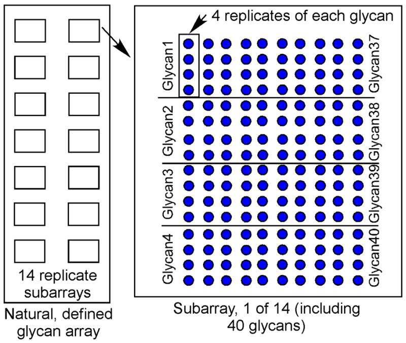
Schematic of natural, defined glycan array printed with 14 identical subarrays per slide. The multi-chamber adaptor can be place over the slide surface to create 14 individual chambers for 14 different, simultaneous assays. In this example, each of the 40 glycans is printed in replicates of 4. In some cases, the printed compounds include controls such as glycopeptides, biotin, etc.

Binding assay for Natural, Defined Glycan Microarray

The principle of the binding assay on the natural glycan microarray is the same as on the CFG glycan microarray, which includes binding, washing, and scanning steps. However, when multiple subarrays are printed on a single slide, the procedure is handled differently. The following protocol uses a biotinylated lectin on a 14-subarray defined glycan microarray format as an example, but it also applies to other printing formats.

For multi-panel experiment on a single slide, a multi-chamber adaptor is fixed on the slide to separate a single slide into 14 chambers sealed from each other during the assay. This allows for multiple assays to be performed simultaneously on up to 14 identical subarrays on the same slide. Sample (for example, biotinylated lectin, 50–100 μL) is applied into each chamber and the incubation is carried out on a shaker at 60 rpm for 1 hour. If some subarrays on one slide are not used, the slide can be saved at −20°C and the unused subarrays can be used at a later time.

Materials

• Biotinylated lectin (commercially available, ex. Vector Labs)

• Alexa Fluor-488-Streptavidin (Invitrogen)

• Natural, defined glycan array printed slides, printed on one side of the slide, 14 identical subarrays per slide

  DO NOT TOUCH THE PRINTED AREA

• Multi-chamber adaptor

• Vacuum suction with clean pipette tips

• Rotating shaker

• 100 ml Coplin jar for washing slides

• Tris-HCl (Fisher Scientific, BP152-1)

• NaCl (Fisher Scientific, S271-3)

• CaCl₂ (Fisher Scientific, C79-500)

• MgCl₂ (Fisher Scientific, BP214-500)

• Potassium Phosphate Monobasic (Fisher Scientific, P285-3)

• dH₂O

• BSA (Fisher Scientific, Bp1600-100)

• Tween-20 (EMD Biosciences, 655205)

• ProScanArray Scanner (Perkin Elmer)

• ScanArray quantitation software (Scanarray Express, Perkin Elmer or Imagene, Biodiscovery)

Buffers (see Basic Protocol 1 for buffer preparation)

• TSM = 20mM Tris-HCl, pH 7.4 150mM NaCl, 2mM CaCl₂, 2mM MgCl₂

• TSM Wash Buffer (TSMWB) = TSM Buffer + 0.05% Tween-20

• TSM Binding Buffer (TSMBB) = TSM buffer + 0.05% Tween-20 + 1% BSA

Protocol

1. Make working stocks of washing buffers (TSM, TSMWB, TSMBB, and H₂O) or collect reagents and bring to room temperature if they have been in the refrigerator.

2. Prepare 100 μl of sample by diluting biotinylated lectin in TSMBB to an appropriate final concentration required for the analysis. For lectins, a beginning concentration of 10 ug/ml should give ample binding, and can be diluted to demonstrate specificity.

3. Remove slide from −20°C and place in a room temperature desiccator to allow slides to warm in a dry environment for at least 30 minutes.

4. Affix multi-chamber adaptor to slide surface.

   DO NOT TOUCH PRINTED AREAS OF SLIDE

5. Hydrate each subarray to be assayed by placing 100 μl of TSMWB in each chamber for 5 minutes at room temperature on the rotating shaker.

6. Remove the TSMWB by vacuum suction or pipetting the liquid out of each chamber.

7. Carefully apply ~100 μl of sample (prepared in step 2) to the appropriate chamber.

8. Cover the chambers with parafilm or a plastic adhesive cover to prevent evaporation during incubation.

9. Incubate slide on the rotating shaker at 60 rpm for 1 hour at room temperature.

10. After 1 hour incubation, remove slide from shaker and remove cover.

11. Remove sample from each chamber by vacuum suction or pipetting.

12. Wash each chamber by adding 200 μl TSMWB 4 times and 200 μl TSM 4 times, removing the buffer after each wash.

13. Add ~100 μl of Streptavidin-AlexaFluor-488 in TSMBB at the appropriate amount (ex. 5 ug/ml) to each chamber.

14. Cover the chambers with parafilm or a plastic adhesive cover.

15. Incubate slide on the rotating shaker for 1 hour at room temperature.

16. After 1 hour incubation, remove slide from shaker and remove cover.

17. Remove sample from each chamber by vacuum suction or pipetting.

18. Wash each chamber by adding 200 μl TSMWB 4 times and 200 μl TSM 4 times, removing the buffer after each wash.

19. Remove the multi-chamber adaptor and rinse the slide in a Coplin jar of 100 mL dH₂O.

20. Spin slide in slide centrifuge for ~ 15 seconds or remove water under a gentle stream of nitrogen.

21. Scan slide with a fluorescent scanner at the appropriate wavelengths

    For Alexa Fluor 488-labeled streptavidin, scan with 488 nm lamp. Save the image.

22. Process the slide with appropriate quantitation software.

Anticipated Results

The data output is essentially the same as that described for CFG glycan microarray. Shown in Figure 4 is an example of biotinylated SNA at 10 μg/ml binding to a natural glycan array comprised of 52 GAEABs as previously described (Song, X., Xia, B., et al. 2009). The structures of the bound glycans are indicated and all possess the NeuAcα2-6Galβ1-4 determinant known to be recognized by SNA.

Figure 4.

The binding of biotinylated SNA to a natural glycan array containing 52 GAEABs and 4 controls. After obtaining a fluorescent image of the biotinylated SNA bound by cyanine5-streptavidin, binding is quantified and displayed as a histogram of the average RFU bound to each glycan. The 8 glycan structures that were bound by SNA are displayed next to their respective peak.

Commentary

Background Information

The specificities of Glycan Binding Proteins (GBPs) can be determined in a high throughput format using microarrays of defined glycans, and the utility of this approach is in direct proportion to the number and variety of the glycans available on the array. A public glycan microarray is available as an investigator-driven resource, where thousands of glycan arrays and been used to analyze hundreds of GBPs. The National Institute for General Medical Sciences (NIGMS) funded the CFG and data are available to the public at http://www.functionalglycomics.org. In this unit we have briefly described protocols generally used by the Glycan Array Synthesis Core (Core D) and the Protein-Glycan Interaction Core (Core H) of the CFG to prepare glycan arrays and interrogate them with GBPs.

Analyzing protein-carbohydrate interactions using assays involving binding of protein to immobilized glycans is a well-established approach; however, the miniaturization of this process to be able to analyze binding of a GBP to hundreds of glycans in a single experiment was an outgrowth of genomic and proteomic analyses based on microarrays, which revolutionized studies of protein-glycan interactions and has resulted in the discovery of new GBP functions (Stowell, S.R., Arthur, C.M., et al. 2010, Stowell, S.R., Arthur, C.M., et al. 2008), new paradigms in anti-glycan antibodies (von Gunten, S., Smith, D.F., et al. 2009), the specificities of anti-glycan antibodies (Luallen, R.J., Agrawal-Gamse, C., et al. 2010), bacterial toxins (Byres, E., Paton, A.W., et al. 2008, Chen C, Fu, Z., et al. 2009, Dingle, T., Wee, S., et al. 2008), plant lectins (Gourdine, J.P., Cioci, G., et al. 2008, Subramanyam, S., Smith, D.F., et al. 2008) and virus binding (Amonsen, M., Smith, D.F., et al. 2007, Kumari, K., Gulati, S., et al. 2007). Natural glycan arrays comprised of glycans tagged with bifunctional fluorescent labels that are suitable for printing on arrays are being developed to expand the repertoire of glycans for interrogating with GBPs.

Critical Parameters, interpreting data, and troubleshooting

Critical parameters, in addition to the necessity of a large number of glycan structures for obtaining quality data from glycan microarrays, include using the appropriate printing techniques for the samples and printing consistent arrays. The purity, diversity, and integrity of the compounds being printed are critical to producing a useful, reliable array. The quality and activity of the GBP being interrogated is also crucial to generating usable data. If the proteins are degraded, inactive, not pure, or are unable to be detected with the chosen detection system, a ‘negative’ or ‘inconclusive’ result could be falsely obtained. Often, unknown factors including inappropriate pH, temperature, incubation time, buffer composition, etc. may contribute to the lack of binding to the glycan array. This can be especially critical with virus samples, which often require 4°C for binding to avoid activity of surface neuraminidase in certain strains, which can remove the sialic acid from the glycans. Some samples may require other cofactors, such as higher amounts of calcium, addition of zinc, or an entirely different buffer or pH. Since the optimal conditions are often not known before testing samples on the array, optimization can be difficult.

Interpreting data is a time-consuming process that requires careful inspection of the bound and unbound structures as well as the relative binding of closely related glycan structures. Evaluation of binding profiles from analyses at decreasing concentrations of GBP are particularly useful in ranking glycans with respect to their relative binding strengths. Such evaluations give a clearer picture of specificity of the GBP interaction. The overall signal intensity can be important, but the relative binding of one glycan to another is often more informative. The degree of variability in binding to a single glycan should be monitored. This variability is measured by calculating the standard deviation of the average of the 4 spots, and the calculated %CV (100 × STDEV/MEAN). If the %CV is high (>20–40%), the results for binding may not be reliable, and if the %CV is >50%, the data should be disregarded. It is unfortunate that in many cases there are no positive controls for a GBP whose glycan binding properties are unknown so a negative result is difficult to interpret. The protein could be inactive or its glycan ligand may not be on the array. Cocktails of lectins with known specificities are use to evaluate the validity of the array, and every printed batch of slides is quality controlled using the cocktail. However, the lectins can also be added to any slide after a negative result is obtained to show that the glycan array itself is not the reason for lack of binding. Control samples for which binding is known on the array (antibodies, etc.) can also be added to confirm that secondary reagents, etc. are in working order. If all parameters on the glycan array are working, then the lack of binding is likely due to sample inactivity, suboptimal conditions, or simply the absence of the glycan-ligand from the tested array. When positive data is seen on the glycan array, it should be further validated by other assays to confirm binding. For example, if a glycan is bound by a GBP, the same glycan structure can be obtained and tested by ELISA to show that the sample can bind the glycan in an alternate format. The glycan array should be viewed as a screening technique and one of several experimental methods to prove the interactions of GBPs with glycan ligands.

Issues related to troubleshooting the printing process are beyond the scope of this unit, but some of the problems associated with analyzing the glycan array include: high background, uneven background, no signal from sample, missing spots (not all of the replicates are showing), no signal from biotin alignment spots, uninterpretable images, and other variables. Table 3 discusses some of these challenges and possible causes and solutions.

Table 3.

Troubleshooting Guide

Problem	Possible cause	Solution(s)
Missing spots or irregular spots	Printer issues- dirty pins or defective tips (capillaries)	Thoroughly clean printing pins or replace capillary tips
	Sample issues- sample is too viscous	Dilute sample, use a different sample buffer
High or uneven slide background	Unsuccessful blocking of slide when printed	Perform blocking step or extend blocking time
	Unsuccessful decrease of background by buffers (Tween, BSA)	Use a higher percent of BSA and/or Tween in the sample buffer
	Drying of the slide during the assay	Keep the slide in a hydration chamber during the assay; use a cover slip over the array; increase the volume of sample on the array
	Insufficient washing steps	Increase the number of wash steps; increase the time of each wash step; change the wash buffers to a more stringent wash
Low signal	Low GBP concentration	Increase amount of GBP; increase the incubation time; increase the incubation temperature;
	Low binding affinity	Decrease wash times; decrease number of washes; use less stringent wash buffers; increase GBP concentration; use more sensitive detection systems
	Problems with detection system	Look for alternate detection systems (direct labeling, different antibody to GBP, pre-complex sample and detection system, etc.)
High imprecision (%CV > 50%)	Poor printing precision	Check printer, increase specifications for quality control
	GBP preparation	Modify buffer pH or ionic strength, detergent concentrations or other parameters to avoid precipitation of protein
Image appears irregular or scarred	Scratched array surface	Use caution to avoid making contact with array surface and remove cover slip gently

Anticipated Results

Glycan microarrays are a new concept in the analysis of protein-carbohydrate interactions and the quality of results may improve as better printing and assay technologies are developed. A key feature is ability to generate a constant array with respect to quantity of glycan printed. Although there is generally some variability in the process of printing hundreds of slides containing hundreds of glycans per slide, analyses are generally carried out on slides from the same printing batch and at several different GBP concentrations to accommodate these variables. The CFG glycan microarray is printed using a contact printer and after more than 5 years of use as a publically available resource, we are unaware of any documented examples of studies of GBP specificities that were mis-assigned based on data from this format. In most cases the assays generate strong signals up to >50,000 Relative Fluorescence Units (RFU) where background (no binding) is close to zero. Specific binding patterns are generally obvious if homogeneous samples and in some cases only a few target glycans with highly related structures are bound by a specific GBP. In cases where binding is low with high imprecision (%CV>30%), the data are classified as inconclusive. Such results are generally associated with inactive protein preparations, problems with the detection systems or absence of the glycan ligand on the array.

Time Considerations

Printing the microarray slides requires the design and layout of the array and the time required will depend on the complexity and number of glycans to be printed, and can take several days to prepare the source plate containing the target glycans. Actual printing time of the defined CFG array containing >500 glycan target at replicates of n=6 using a contact printer is a matter of hours and including the reaction time, blocking and washing steps 100 slides can be produced and 2 to 3 days. Piezo-electronic printing, which is limited by the availability of only 4 to 8 capillaries, requires significantly more time. For example, 5 slides printed with 14 subarrays of 100 glycan targets in replicates of 4 requires about 8 hours. Thus, including the reaction time, blocking and washing steps, 5 slides (70 arrays) can be produced in 2 to 3 days. The quality control steps can take 1–3 days, depending on the number of different controls being used to ensure the quality of the slides.

The assay time on the printed slides varies by the type of sample and the method of detection. For directly labeled samples that require only a 1 hour incubation, as described for a labeled virus, the total assay time is only about 2 hours. For each additional step that is needed (for example, 1 additional step for monoclonal antibodies), about 1 hour 30 minutes can be added to the 2 hours. Analysis of the fluorescent signal in the scanning equipment requires only a few minutes for actual scanning, but the analysis of the image can take some time depending on the quality and quantity of signal obtained. In most analysis software the spots must be aligned to the grid manually, followed by quantitation of the amount of signal. An average analysis time is about 30 minutes per slide. Once the data are processed to histograms and tables of structures ranked in order of binding strengths to look for patterns of binding or glycan-binding motifs. Considerable time is required for inspecting the glycan structures and comparing the relative binding strengths of related structures and comparing them to the structures that were not bound. This process can also be lengthy depending on the complexity of the output, but is necessary to define an accurate binding motif.

References

- Amonsen M, Smith DF, et al. Human parainfluenza viruses hPIV1 and hPIV3 bind oligosaccharides with alpha2-3-linked sialic acids that are distinct from those bound by H5 avian influenza virus hemagglutinin. J Virol. 2007;81:8341–8345. doi: 10.1128/JVI.00718-07. [DOI] [PMC free article] [PubMed] [Google Scholar]
- Blixt O, Head S, et al. Printed covalent glycan array for ligand profiling of diverse glycan binding proteins. Proc Natl Acad Sci U S A. 2004;101:17033–17038. doi: 10.1073/pnas.0407902101. [DOI] [PMC free article] [PubMed] [Google Scholar]
- Bohorov O, Andersson-Sand H, et al. Arraying glycomics: a novel bi-functional spacer for one-step microscale derivatization of free reducing glycans. Glycobiology. 2006;16:21C–27C. doi: 10.1093/glycob/cwl044. [DOI] [PubMed] [Google Scholar]
- Byres E, Paton AW, et al. Incorporation of a non-human glycan mediates human susceptibility to a bacterial toxin. Nature. 2008;456:648–652. doi: 10.1038/nature07428. [DOI] [PMC free article] [PubMed] [Google Scholar]
- Chen C, Fu Z, et al. Gangliosides as high affinity receptors for tetnus neurotoxin. J Biol Chem. 2009;284:26569–26577. doi: 10.1074/jbc.M109.027391. [DOI] [PMC free article] [PubMed] [Google Scholar]
- Connor RJ, Kawaoka Y, et al. Receptor specificity in human, avian, and equine H2 and H3 influenza virus isolates. Virology. 1994;205:17–23. doi: 10.1006/viro.1994.1615. [DOI] [PubMed] [Google Scholar]
- Cummings RD. The repertoire of glycan determinants in the human glycome. Mol Biosyst. 2009;5:1087–1104. doi: 10.1039/b907931a. [DOI] [PubMed] [Google Scholar]
- de Boer AR, Hokke CH, et al. General microarray technique for immobilization and screening of natural glycans. Anal Chem. 2007;79:8107–8113. doi: 10.1021/ac071187g. [DOI] [PubMed] [Google Scholar]
- Dingle T, Wee S, et al. Functional properties of the carboxy-terminal host cell-binding domains of the two toxins, TcdA and TcdB, expressed by Clostridium difficile. Glycobiology. 2008;18:698–706. doi: 10.1093/glycob/cwn048. [DOI] [PubMed] [Google Scholar]
- Disney MD, Seeberger PH. The use of carbohydrate microarrays to study carbohydrate-cell interactions and to detect pathogens. Chem Biol. 2004;11:1701–1707. doi: 10.1016/j.chembiol.2004.10.011. [DOI] [PubMed] [Google Scholar]
- Elkins RP. Multi-analyte immunoassua. Journal of Pharmaceutical & Biomedical Analysis. 1989;7:155–168. doi: 10.1016/0731-7085(89)80079-2. [DOI] [PubMed] [Google Scholar]
- Feizi T, Fazio F, et al. Carbohydrate microarrays - a new set of technologies at the frontiers of glycomics. Curr Opin Struct Biol. 2003;13:637–645. doi: 10.1016/j.sbi.2003.09.002. [DOI] [PubMed] [Google Scholar]
- Feizi T, Stoll MS, et al. Neoglycolipids: probes of oligosaccharide structure, antigenicity, and function. Methods Enzymol. 1994;230:484–519. doi: 10.1016/0076-6879(94)30030-5. [DOI] [PubMed] [Google Scholar]
- Gildersleeve JC, Oyelaran O, et al. Improved procedure for direct coupling of carbohydrates to proteins via reductive amination. Bioconjug Chem. 2008;19:1485–1490. doi: 10.1021/bc800153t. [DOI] [PMC free article] [PubMed] [Google Scholar]
- Gourdine JP, Cioci G, et al. High affinity interaction between a bivalve C-type lectin and a biantennary complex-type N-glycan revealed by crystallography and microcalorimetry. J Biol Chem. 2008;283:30112–30120. doi: 10.1074/jbc.M804353200. [DOI] [PMC free article] [PubMed] [Google Scholar]
- Hardman KD, Ainsworth CF. Structure of concanavalin A at 2.4-A resolution. Biochemistry. 1972;11:4910–4919. doi: 10.1021/bi00776a006. [DOI] [PubMed] [Google Scholar]
- Heller MJ. DNA microarray technology: devices, systems, and applications. Annu Rev Biomed Eng. 2002;4:129–153. doi: 10.1146/annurev.bioeng.4.020702.153438. [DOI] [PubMed] [Google Scholar]
- Kramer S, Joos TO, Templin MF. Protein Microarrays. Current Protocols in Protein Science. 2005;23:23.25.21–23.25.20. doi: 10.1002/0471140864.ps2305s39. [DOI] [PubMed] [Google Scholar]
- Krishnamurthy VR, Wilson JT, et al. Chemoselective Immobilization of Peptides on Abiotic and Cell Surfaces at Controlled Densities. Langmuir. 2010 doi: 10.1021/la101192v. [DOI] [PMC free article] [PubMed] [Google Scholar]
- Kulesh DA, Clive DR, et al. Identification of interferon-modulated proliferation-related cDNA sequences. Proc Natl Acad Sci U S A. 1987;84:8453–8457. doi: 10.1073/pnas.84.23.8453. [DOI] [PMC free article] [PubMed] [Google Scholar]
- Kumari K, Gulati S, et al. Receptor binding specificity of recent human H3N2 influenza viruses. Virol J. 2007;4:42. doi: 10.1186/1743-422X-4-42. [DOI] [PMC free article] [PubMed] [Google Scholar]
- Liu Y, Feizi T, et al. Neoglycolipid probes prepared via oxime ligation for microarray analysis of oligosaccharide-protein interactions. Chem Biol. 2007;14:847–859. doi: 10.1016/j.chembiol.2007.06.009. [DOI] [PubMed] [Google Scholar]
- Luallen RJ, Agrawal-Gamse C, et al. Antibodies against Manalpha1,2-Manalpha1,2-Man oligosaccharide structures recognize envelope glycoproteins from HIV-1 and SIV strains. Glycobiology. 2010;20:280–286. doi: 10.1093/glycob/cwp184. [DOI] [PMC free article] [PubMed] [Google Scholar]
- Luyai A, Lasanajak Y, et al. Facile Preparation of Fluorescent Neoglycoproteins Using p-Nitrophenyl Anthranilate as a Heterobifunctional Linker. Bioconjug Chem. 2009 doi: 10.1021/bc900189h. [DOI] [PMC free article] [PubMed] [Google Scholar]
- Oyelaran O, Li Q, et al. Microarrays with varying carbohydrate density reveal distinct subpopulations of serum antibodies. J Proteome Res. 2009;8:3529–3538. doi: 10.1021/pr9002245. [DOI] [PMC free article] [PubMed] [Google Scholar]
- Park S, Lee MR, et al. Fabrication of carbohydrate chips and their use to probe protein-carbohydrate interactions. Nat Protoc. 2007;2:2747–2758. doi: 10.1038/nprot.2007.373. [DOI] [PubMed] [Google Scholar]
- Park S, Lee MR, et al. Construction of carbohydrate microarrays by using onestep, direct immobilizations of diverse unmodified glycans on solid surfaces. Bioconjug Chem. 2009;20:155–162. doi: 10.1021/bc800442z. [DOI] [PubMed] [Google Scholar]
- Park S, Shin I. Fabrication of carbohydrate chips for studying protein-carbohydrate interactions. Angew Chem Int Ed Engl. 2002;41:3180–3182. doi: 10.1002/1521-3773(20020902)41:17<3180::AID-ANIE3180>3.0.CO;2-S. [DOI] [PubMed] [Google Scholar]
- Pollack JR. DNA microarray technology. Introduction. Methods Mol Biol. 2009;556:1–6. doi: 10.1007/978-1-60327-192-9_1. [DOI] [PubMed] [Google Scholar]
- Ramsay G. DNA chips: state-of-the art. Nat Biotechnol. 1998;16:40–44. doi: 10.1038/nbt0198-40. [DOI] [PubMed] [Google Scholar]
- Ratner DM, Adams EW, et al. Probing protein-carbohydrate interactions with microarrays of synthetic oligosaccharides. Chembiochem. 2004;5:379–382. doi: 10.1002/cbic.200300804. [DOI] [PubMed] [Google Scholar]
- Rogers GN, D’Souza BL. Receptor binding properties of human and animal H1 influenza virus isolates. Virology. 1989;173:317–322. doi: 10.1016/0042-6822(89)90249-3. [DOI] [PubMed] [Google Scholar]
- Song X, Lasanajak Y, et al. Generation of a natural glycan microarray using 9-fluorenylmethyl chloroformate (FmocCl) as a cleavable fluorescent tag. Anal Biochem. 2009;395:151–160. doi: 10.1016/j.ab.2009.08.024. [DOI] [PMC free article] [PubMed] [Google Scholar]
- Song X, Lasanajak Y, et al. Fluorescent glycosylamides produced by microscale derivatization of free glycans for natural glycan microarrays. ACS Chem Biol. 2009;4:741–750. doi: 10.1021/cb900067h. [DOI] [PMC free article] [PubMed] [Google Scholar]
- Song X, Xia B, et al. Quantifiable fluorescent glycan microarrays. Glycoconj J. 2008;25:15–25. doi: 10.1007/s10719-007-9066-8. [DOI] [PubMed] [Google Scholar]
- Song X, Xia B, et al. Novel fluorescent glycan microarray strategy reveals ligands for galectins. Chem Biol. 2009;16:36–47. doi: 10.1016/j.chembiol.2008.11.004. [DOI] [PMC free article] [PubMed] [Google Scholar]
- Stevens J, Blixt O, et al. Glycan microarray analysis of the hemagglutinins from modern and pandemic influenza viruses reveals different receptor specificities. J Mol Biol. 2006;355:1143–1155. doi: 10.1016/j.jmb.2005.11.002. [DOI] [PubMed] [Google Scholar]
- Stoll MS, Feizi T, et al. Fluorescent neoglycolipids. Improved probes for oligosaccharide ligand discovery. Eur J Biochem. 2000;267:1795–1804. doi: 10.1046/j.1432-1327.2000.01178.x. [DOI] [PubMed] [Google Scholar]
- Stowell SR, Arthur CM, et al. Innate immune lectins kill bacteria expressing blood group antigen. Nat Med. 2010;16:295–301. doi: 10.1038/nm.2103. [DOI] [PMC free article] [PubMed] [Google Scholar]
- Stowell SR, Arthur CM, et al. Dimeric Galectin-8 induces phosphatidylserine exposure in leukocytes through polylactosamine recognition by the C-terminal domain. J Biol Chem. 2008;283:20547–20559. doi: 10.1074/jbc.M802495200. [DOI] [PMC free article] [PubMed] [Google Scholar]
- Subramanyam S, Smith DF, et al. Functional characterization of HFR1, a high-mannose N-glycan-specific wheat lectin induced by Hessian fly larvae. Plant Physiol. 2008;147:1412–1426. doi: 10.1104/pp.108.116145. [DOI] [PMC free article] [PubMed] [Google Scholar]
- Varki A, Cummings RD, et al. Essentials of Glycobiology. Cold Spring Harbor Laboratory Press; Cold Spring Harbor, N.Y: 2009. [PubMed] [Google Scholar]
- von Gunten S, Smith DF, et al. Intravenous immunoglobulin contains a broad repertoire of anticarbohydrate antibodies that is not restricted to the IgG2 subclass. J Allergy Clin Immunol. 2009;123:1268–1276. e1215. doi: 10.1016/j.jaci.2009.03.013. [DOI] [PMC free article] [PubMed] [Google Scholar]