

Abstract
Projection data incompleteness arises in many situations relevant to X-ray computed tomography (CT) imaging. We propose a penalized maximum likelihood statistical sinogram restoration approach that incorporates the Helgason–Ludwig (HL) consistency conditions to accommodate projection data incompleteness. Image reconstruction is performed by the filtered-backprojection (FBP) in a second step. In our problem formulation, the objective function consists of the log-likelihood of the X-ray CT data and a penalty term; the HL condition poses a linear constraint on the restored sinogram and can be implemented efficiently via fast Fourier transform (FFT) and inverse FFT. We derive an iterative algorithm that increases the objective function monotonically. The proposed algorithm is applied to both computer simulated data and real patient data. We study different factors in the problem formulation that affect the properties of the final FBP reconstructed images, including the data truncation level, the amount of prior knowledge on the object support, as well as different approximations of the statistical distribution of the available projection data. We also compare its performance with an analytical truncation artifacts reduction method. The proposed method greatly improves both the accuracy and the precision of the reconstructed images within the scan field-of-view, and to a certain extent recovers the truncated peripheral region of the object. The proposed method may also be applied in areas such as limited angle tomography, metal artifacts reduction, and sparse sampling imaging.
Index Terms: Computed tomography (CT) artifacts, fan beam computed tomography, image reconstruction, incomplete projection
I. Introduction
Different kinds of projection data incompleteness arise in various situations in X-ray computed tomography (CT). When the patient body extends outside of the scanner field-of-view (SFOV), the projection data will be truncated in the transverse direction. Radiation dose concerns may also lead to reduced scan schemes so that a small region-of-interest is fully enclosed in the SFOV while other organs are truncated. If not properly treated, data truncation produces edge and cupping artifacts near the edge of SFOV that obscure the underlying anatomy and make diagnosis difficult [1].
In iterative image reconstruction algorithms that use repeated forward and backward projections, projection incompleteness can be included as part of the system matrix modeling. Two different approaches for treating the missing projection rays, ignore or estimate, were proposed in [2] and [3] that resulted in the same fixed point in their respective maximum-likelihood estimation algorithms. The observation was that, if the reconstruction volume is big enough to cover the scanned object [3], [4], then projection incompleteness is taken care of by the system geometry modeling, thus artifacts caused by data incompleteness can be reduced.
Despite their capability of dealing with truncation and many other artifacts, the high computational cost of iterative reconstruction methods nowadays prevents their routine application in clinical X-ray CT practice. The algorithm-of-choice on commercial CT scanners is still the filtered-backprojection (FBP) type analytical reconstruction algorithms. If the truncated projection data are directly fed to these algorithms, the abrupt change of projection values at the edge of SFOV causes significant artifacts in the reconstructed images [1]. A projection data completion method is a preprocessing step for obtaining a complete projection data, so that subsequent FBP reconstruction can have reduced artifacts within the SFOV, and extend the reconstruction field-of-view (RFOV) beyond the SFOV [5], [6].
It is well known that the sinogram of a physical function cannot be arbitrary and satisfies the so-called consistency conditions [7], [8], which essentially characterize the range of the Radon transform. In the interest of this work, we divide the different projection data completion methods into two categories. The first category takes an extrapolation approach without explicit use of consistency conditions, such as the minimal value extension method in [9] and [10] and the symmetric mirroring method in [6]. The second category [5], [11]–[14] makes use of consistency conditions. Among these, [5], [11] use the first order consistency condition (constant body mass) to constrain the data extrapolation procedure. In [12] a new fan beam data consistency condition was derived and the missing projection values were filled in point-by-point in an iterative manner. There are pros and cons in the two categories. Since the consistency conditions are most conveniently employed in the parallel beam geometry, fan-to-parallel rebinning is usually needed for the second category of methods, while in the first category the projection extrapolation or data extension can be performed in the native geometry. However without incorporating the consistency conditions, extrapolation tends to be ad-hoc and usually relies on local continuity conditions at the edge of the SFOV. They may also require various thresholds settings that may not be straightforward when the imaging condition changes, e.g., high dose versus low dose applications.
Two approaches [13], [14] in the second category explicitly use the Helgason–Ludwig [7], [8] consistency condition1 and expand the Radon transform in terms of its basis functions [15, Ch. IV and equation (3.13)]. Their methods therefore incorporate not just one or two consistency conditions as in [5], [6], but theoretically an infinite number of such constraints [14]. Our proposed method builds on these previous works and extends the methodology to data completion problems in X-ray CT imaging.
We develop a statistical sinogram restoration method for X-ray CT that incorporates 1) the noise statistics of the X-ray CT data, and 2) the HL consistency condition to deal with projection data incompleteness. The recovered sinogram is subsequently reconstructed by the analytical FBP type algorithms. We compare our results with direct FBP reconstruction with no correction and after projection completion using the symmetric mirroring method [6], an ad-hoc data extrapolation approach that tries to recover the truncated projection values from those available data in a certain mirroring manner. Our comparison demonstrates both improved accuracy and precision of the object attenuation coefficients within the SFOV.
Though all make explicit use of the HL condition and are formulated as a sinogram restoration approach, there are significant differences among [13], [14], and our method, in terms of 1) the problem formulation, 2) algorithm derivation, and 3) procedures to enforce the HL condition. In [13], the complete sinogram was determined by satisfying some prescribed desirable properties, e.g., consistency, known sinogram support, and a priori knowledge of a reference sinogram, that are formulated as convex sets. A POCS algorithm was used to find the solution iteratively. In [14] a different set of basis functions were used and the HL condition was cast as hard constraints by forcing some basis expansion coefficients of the sinogram to be zero. In their iterative scheme, these hard constraints were incorporated into a penalized least squares objective function by introducing Lagrange multipliers. A primal-dual type algorithm was implemented to find the optimizer [14].
We consider the noise statistics of the X-ray CT projection and formulate the sinogram restoration problem in the penalized maximum-likelihood framework. By borrowing the linear representation from [13], the HL condition is again posed as a linear condition on the solution sinogram. This formulation makes the algorithm derivation easier without using Lagrange multipliers. In different X-ray CT applications, the projection data can either be in the pre-log operation format, or in the after-log operation format. We look at two separate statistical assumptions of the X-ray projection data for the two situations, a Poisson model and a Gaussian model. We derive an iterative algorithm that monotonically increases the objective function by using the optimization transfer principle [16], [17]. Moreover, enforcing the HL condition is achieved by fast Fourier transform (FFT) and inverse FFT (IFFT).
The organization of this paper is as follows. For completeness, in Section II we first introduce the HL condition following the exposition of [13] and [14] and explain how the sinogram series expansion can be calculated via FFT. In Section III we present our sinogram restoration problem with explicit incorporation of the HL condition and derive an iterative algorithm that monotonically increases a penalized likelihood function. Reconstruction results using computer simulated data and real patient acquisitions are presented and analyzed in Sections IV and VI. We also compare results from our proposed approach with that from the symmetric mirroring method [6]. We conclude this paper and discuss possible extensions of this work in Section VII. In Table I below we assemble some notations from [15] related to the 2-D Radon transform.
TABLE I.
2-D Radon Transform Notations
| S, Ω2 | unit circle, unit disk of R2 |
| Z = S × R | unit cylinder of R3 |
| L2 (Ω) | space with norm (∫Ω|f|2 dx)1/2 |
| L2 (Ω, w) | same as L2(Ω) but with the weight w |
II. Background
The HL condition is part of our sinogram restoration problem formulation. In this section, we first introduce the HL condition of the 2-D Radon transform, which states that some of the series expansion coefficients of the 2-D Radon transform must be zero for it to be physically possible. For the purpose of efficient algorithm implementation, we then explain how the series expansion coefficients and the 2-D Radon transform are related by Fourier transform pair.
A. Helgason–Ludwig Consistency Conditions
With occasional exceptions, our notations here are almost identical to those in [13]. The interested readers are referred to [13], [14] for more information. We denote by
 the 2-D Radon transform that maps the Hilbert space L2(Ω)2 to L2(Z, (1 − r2)−1/2), −1 ≤ r < 1. Any physically consistent sinogram g(r, θ) can then be written as a series expansion using the basis functions of L2(Z, (1 − r2)−1/2)
| (1) |
where −1 ≤ r < 1 and 0 ≤ θ < 2π. The complex constants bkm are the expansion coefficients. The function Uk(r) is the kth order Chebyshev polynomial of the second kind. Let g1, g2 ∈ L2(Z, (1 − r2)−1/2), the inner product of g1 and g2 is defined as follows:
| (2) |
The functions form an orthogonal basis of L2(Z, (1 − r2)−1/2). The HL consistency condition dictates that not all expansion coefficients bkm can be arbitrary. In fact, the HL condition is embodied in the following requirement on bkm [13]:
| (3) |
Let ĝ(r, θ) ∉ Range(
), then some of its expansion coefficients bkm violate the HL condition (3). We use the notation [b]r to denote the operation of zeroing out these “inconsistent” coefficients; the resulting sinogram ǧ(r, θ) obtained by plugging the “rectified” expansion coefficients [b]r into (1) satisfies
| (4) |
such that g(r, θ) ∈ Range(
).
B. Sinogram Series Expansion Using FFT
If we define
| (5) |
then (1) can be rewritten as
| (6) |
In other words, hm(r) are the coefficients of the Fourier series expansion of g(r, θ) with respect to θ. The conversion of g(r, θ) ↔ hm(r) therefore can be implemented via 1D FFT along the view direction. The transformation between hm(r) and bkm in (5) can be calculated by a discrete sine transform [18], [19]. The key is to utilize the following definition of the Chebyshev polynomial Uk(r):
and realize that by resampling hm(r), −1 < r < 1 at r = cos γ, 0 ≤ γ < π we then have
| (7) |
To complete qm(γ) as a periodic function in γ, we may define
| (8) |
The coefficients bkm can then be obtained from a discrete sine transform of qm(γ), a resampled version of hm(r). For the convenience of our algorithm description, we use the phrase “sinogram expansion” to indicate the calculation of g(r, θ) → bkm; and “sinogram synthesis” the reverse direction. Combining (6), (7), and (8), sinogram expansion can be achieved via fast Fourier transform (FFT), first along the channel direction (r), then along the view direction (θ). The reverse direction, sinogram synthesis, can be achieved via inverse FFT. For g(r, θ) ∈ Range(
), its expansion coefficients bkm necessarily satisfy the HL condition in (3). Conversely, if some of the conditions in (3) are violated, the synthesized “sinogram” from such bkm’s can not be consistent with any physical objects.
III. Methods
In this section, we formulate the sinogram restoration problem in the discrete sinogram space incorporating the HL consistency conditions. To connect with the continuous space description of the HL condition and the sinogram series expansion in Section II, we first discretize the series expansion of Section II and obtain in Section III-A a discrete, linear operator form describing the HL consistency condition, based on which we present our problem definition in Section III-B. In Section III-C we provide a flowchart of the iterative sinogram restoration algorithm, the derivation of which is given in Appendix A. Our problem formulation and algorithm implementation distinguish two index sets,
 and
and
 , the combination of which forms the index set of a complete sinogram, the output of our sinogram completion algorithm. In Section III-E, we use an example to describe the relationship between a truncated sinogram and the index sets
,
, and explain how they can be determined or estimated prior to sinogram restoration.
, the combination of which forms the index set of a complete sinogram, the output of our sinogram completion algorithm. In Section III-E, we use an example to describe the relationship between a truncated sinogram and the index sets
,
, and explain how they can be determined or estimated prior to sinogram restoration.
A. An Operator Form of the HL Condition
Using qm(γ) in (7) as the Fourier series coefficients, we define a “resampled” version of the sinogram g(r, θ) along the channel direction as the following:
| (9) |
Our projection completion procedure is applied to a discretized version of q(γ, θ) rather than g(r, θ). The convenience of working with q(γ θ) is mainly computational as q(γ, θ) and bkm are related by the Fourier transform pair. Note that q(γ, θ) is a 2π periodic function in both γ and θ; only half of it, defined on γ: [0, π) × θ: [0, 2π) corresponds to a resampled version of the sinogram g(r, θ).
To formulate our sinogram restoration problem, in the rest of the paper we use a discrete linear operator form for (9) as
| (10) |
The right-hand side vector b is a concatenation of the basis coefficients b = [···, bkm, ···]T which includes both the “consistent” and the “inconsistent” parts; the kmth column of the Q matrix is the vector qkm = [···, sin((k+1)γu)exp{jmθv}, ···]T, u = 1, ···, U, and v = 1, ···, V, listed in a lexicographical order. The non-subscripted variable l = [···, li, ···]T represents the discretized version of q(γ, θ). For each i, li = q(γu, θv) for a pair of specific γu and θv. With proper normalization, it is easy to see from (9) that QTQ = I, the identity operator.
Let ĝ(r, θ) ∉ Range (
), then a consistent sinogram g(r, θ) ∈ Range (
) that minimizes (4) can be equivalently obtained from q̂ (γ, θ) and q(γ, θ), respectively the cosine-resampled versions of ĝ(r, θ) and g(r, θ) at r = cosγ, by minimizing the following function:
| (11) |
instead. Both involve zeroing-out the “inconsistent” coefficients bkm that violates the HL condition (3). The solution to (11) can be described concisely by q = Q[QTq̂]r, where QT represents sinogram expansion using FFT, and Q sinogram synthesis by inverse FFT.
Unfortunately, minimizing (4) or (11) does not provide a satisfying solution to the projection completion problem. The incomplete projection data ĝ(r, θ) are usually padded with zeros to fill in the missing region. The solution to (4) and (11) is a closest match, in their respective (weighted) least squares sense, to ĝ(r, θ) regardless of whether the match takes place in the measured region of ĝ(r, θ), or over regions that we artificially pad with zeros. A more satisfying solution should be one such that the good match only takes place in those “trusted” region, over the missing region the solution g(r, θ)should assume some consistent values but not seek agreement with those padded zeros. Next we formulate a statistical sinogram restoration problem and define the “good” match, the “trust” region, and consistency in a precise manner.
B. Statistical Projection Completion Using Consistency Conditions
Following [3], we denote the index set of an ideal (complete) set of measurements by
 , the available2 but incomplete set of measurements
, and their difference, the missing portion by
=
\
.
, the available2 but incomplete set of measurements
, and their difference, the missing portion by
=
\
.
We model the transmission CT data yi as Possion distributed random variables with mean Yi = die−li, i ∈
, where di is the air scan intensity at the detector cell i, and li is the unknown line integral of attenuation coefficients from the X-ray source to the ith detector cell. The measured (incomplete) data yi available for i ∈
. Our sinogram restoration algorithm is then formulated as the following:
| (12a) |
| (12b) |
| (12c) |
The objective function in (12) consists of two terms. The first term in (12a) represents the Poisson log-likelihood of the available incomplete data. The second term (12b) represents a smoothness penalty defined for all i ∈
. The constant β > 0 is a penalization weighting that controls the overall strength of smoothing. In this work, we use the quadratic penalty function [20] that penalizes abrupt changes in li
| (13) |
where Ni consists of the neighborhood pixels of the pixel i. For a nonboundary pixel i, we penalize the horizontal (channel direction) and vertical (view direction) differences in the sinogram similar to [20], i.e., a neighborhood of four pixels of equal weights. The constraints in (12c) requires that the restored sinogram li, i ∈
must obey the HL condition. Subject to this constraint, the objective function seeks to maximize the penalized data log-likelihood when the data are available; when they are not, the sinogram restoration relies on the local smoothness penalty. The unknowns in our problem formulation (12) are li, i ∈
, the known input data are di, yi, i ∈
.
As written in (12c), the “effective” unknowns are those free basis coefficients bkms that are allowed to be nonzero under the HL consistency condition. We may partition the vector b as , the free parts bf and the a priorily zero parts (for consistent sinograms) bz, then . If we similarly partition Q = [Qf|Qz], then the expression in (12c) is equivalent to l = Qfbf. The unknowns of our sinogram restoration problem are the bf’s. The expression in (12c) emphasizes that the computation of bf can be achieved via FFT, which necessarily involves bz but does not affect the result of bf.
If we treat the constraint in (12c) as a generic linear operator rather than the HL condition, the problem formulation of (12) is similar to a fully iterative reconstruction problem in transmission CT imaging [21]. Some considerations are called for if we attempt to follow the derivation of a “reconstruction” algorithm for b as that in [21] and [22]. First, in the problem statement of (12), both the unknowns b and the “system” matrix Q are made of complex numbers, whereas in a reconstruction problem these are all nonnegative real numbers. Second, a sequential updating scheme such as the one in [21] may not fully exploit the particular structure of Q embodying the HL condition. An efficient implementation of the “projection” Q and “backprojection” operator QT (in the language of fully iterative reconstruction techniques) is critical for our sinogram restoration algorithm. In the Appendix we derive an iterative algorithm for updating b and hence l of the problem in (12) that uses FFT and IFFT we described in Section II-B to perform the forward and backward projection operations Q and QT, respectively. Starting from a certain consistent sinogram , the update equations for b− can be symbolically expressed as follows:
| (14a) |
| (14b) |
where F(l) is a column vector and Λ(l) is a negative-definite diagonal matrix. Their exact expressions are derived in Appendix A. The constant α is a fixed relaxation parameter, α = 1/maxi[−λi(li)] > 0.
C. Reconstruction From Incomplete Projections
Combining the contents of the previous sections, a flowchart of our proposed statistical projection completion algorithm can be described as follows.
Zero-pad channels so that theRFOV ⊇ SFOV.
Fan-to-parallel beam rebinning.
Cosine transform along the channel direction.
- Initialization.
-
Do {
Calculate l−, F (l−) and Λ(l−).
-
Update b− according to (14).
} Until convergence criterion is met.
Arc-cosine transform along the channel direction.
Parallel beam FBP reconstruction.
To extend the RFOV beyond the SFOV, we first zero-pad a number of channels to the projection data matrix; this step may require a priori knowledge of the size and shape of the scanned object. Secondly, we perform fan beam to parallel beam rebinning for application of the HL condition. The third step is to implement the cosine re-sampling operation in (7) so that enforcing the HL condition can be implemented by FFT and IFFT as explained in Section III-A. A natural initialization scheme of l0 is to fill it with the direct estimate of the line integrals where they are available, i.e., i ∈
and zero elsewhere, i.e., i ∈
. However such an initial estimate is not a consistent sinogram, therefore some rectification is needed as indicated in Step 4. From this point the iteration starts (Step 5). We apply the positivity constraint after sinogram synthesis to ensure l− ≥ 0. This helps to reduce the numerical error accumulation in the repeated FFTs.
The stopping criterion we used in this work is either a maximum of 2000 iterations or , the sum of the absolute difference between consecutive updates is less than 1, whichever is met first. From the l− at the last iteration, we perform arc-cosine transform along the channel direction to come back to the sinogram domain, and apply FBP for parallel beam geometry to obtain the final reconstructed image.
D. Weighted Least Squares Formulation
In a clinical environment, the raw data we can obtain from an X-ray CT scanner are preprocessed line integrals. An alternative problem formulation is the following weighted least squares objective function subject to the HL consistency condition:
| (15) |
where l̂i’s are the acquired line integral data, the least squares weighting term can be taken as the variance of l̂i. If l̂i = log di/yi, and yi is Poisson with mean Ȳi = die−li, then can be approximated by 1/yi [23]. An update equation for b and l can be obtained similar to Section III-B. Please see Appendix B.
Both the Poisson model (12) and the Gaussian model (15) for a statistical formulation of low dose X-ray CT imaging have been proposed in the literature [24], [25]. They are both approximate since the detection and the preprocessing of raw data in a clinical scanner is complicated and therefore approximation is necessary. One of our simulation studies will be to compare the properties of the final FBP reconstructed images using the two models in (12) and (15), in order to empirically evaluate the effects of different approximations in our particular problem setting.
E. Obtaining
and
As a first step of the sinogram completion procedure, the truncated projection is padded with zeros to enlarge the RFOV (Section III-C, flowchart). The index sets
and
are defined on the padded sinogram and their estimates can be obtained from the forward projection of the object boundary (support) information (Fig. 1). If truncation is mild, the direct FBP image using the truncated projection data can provide an estimate of the object support; otherwise some a priori knowledge of the object size may be necessary. This object support is then forward projected, the parts that project to the extend projection region are marked as
, and the other regions, i.e., everything measured plus parts of the extended region where the object supports does not project to,
. In other words,
=
∪
is the complete sinogram that can be applied directly to FBP. If i ∈
, the corresponding yi is not acquired (missing). If i ∈
, the corresponding yi is either measured but noisy, or not measured but is assured to be zero from an estimated object support.
Fig. 1.
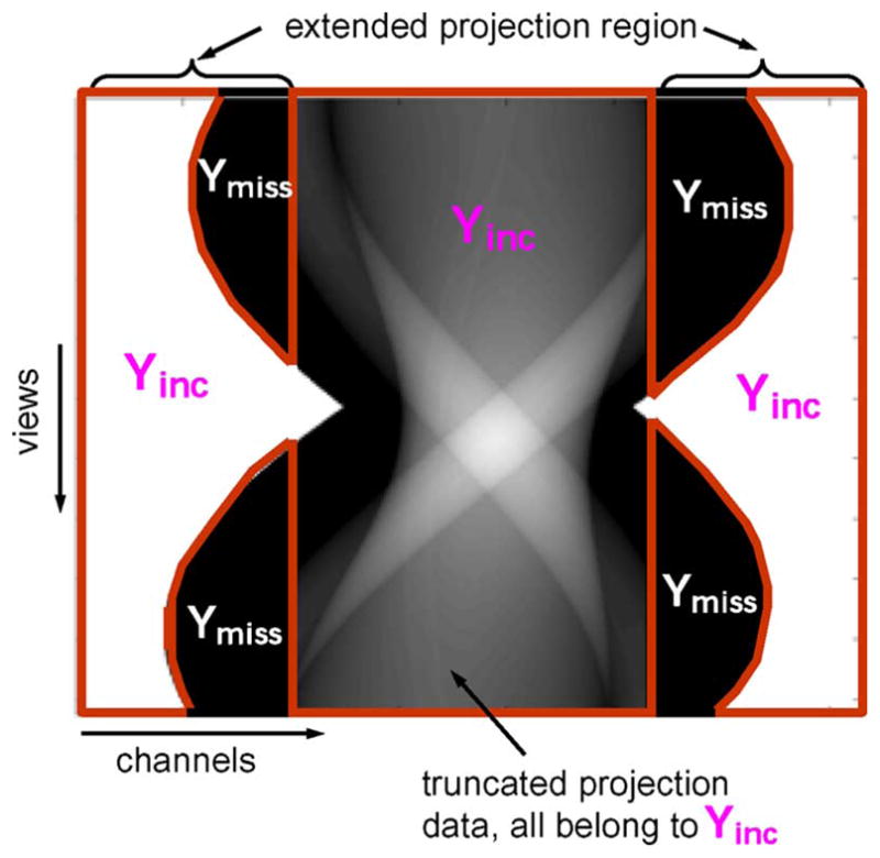
The truncated projection data (after log operation) and its relationship with
and
.
is obtained from the forward projection of an object support estimate. A loose object support estimate is used in this example.
A question then naturally arises as how much the object boundary estimate affects the reconstructed images within the SFOV and within the RFOV. To answer the question, we study the performance of the proposed sinogram completion algorithm using three object support estimates, i.e., an exact object boundary, a tight estimate, and a loose estimate in our simulation studies.
IV. Computer Simulations and Evaluation Methods
We investigated three factors that may affect the performance of our proposed algorithm: 1) the severeness of truncation, 2) the accuracy of the object support estimation, and 3) the regularization weight β and different statistical approximations of the projection data.
We used a digital phantom that mimics the human torso anatomy (Fig. 2) and simulated parallel beam projection data first without truncation. To avoid sampling symmetry, this phantom was placed tilted and offset (by 2.5 cm in both x and y direction) from the iso-center of a simulated SFOV of 50 cm. The maximum line integral is around 9 along the long-axis of the phantom. A high density pin was inserted in the lung region to measure the resolution properties in the FBP reconstructed images using different projection completion methods. A selected number t of boundary channels in the projection image were then set to zero [Fig. 3(a)] simulating transverse truncation. The line integrals of attenuation coefficients were exponentiated and scaled by the uniform air scan intensity of 108, 107, 106 for different noise levels. Poisson perturbation was then introduced to projection data based on the mean transmitted counts in each detector cell. Noise-free projection data with the high density pin present, and Poisson distributed noisy data without the high density pin were separately simulated. Twenty independent noise realizations were generated in order to calculate the mean profiles and standard deviations. In the next three subsections, we describe the simulation studies and the evaluation methods for each of the above three factors.
Fig. 2.
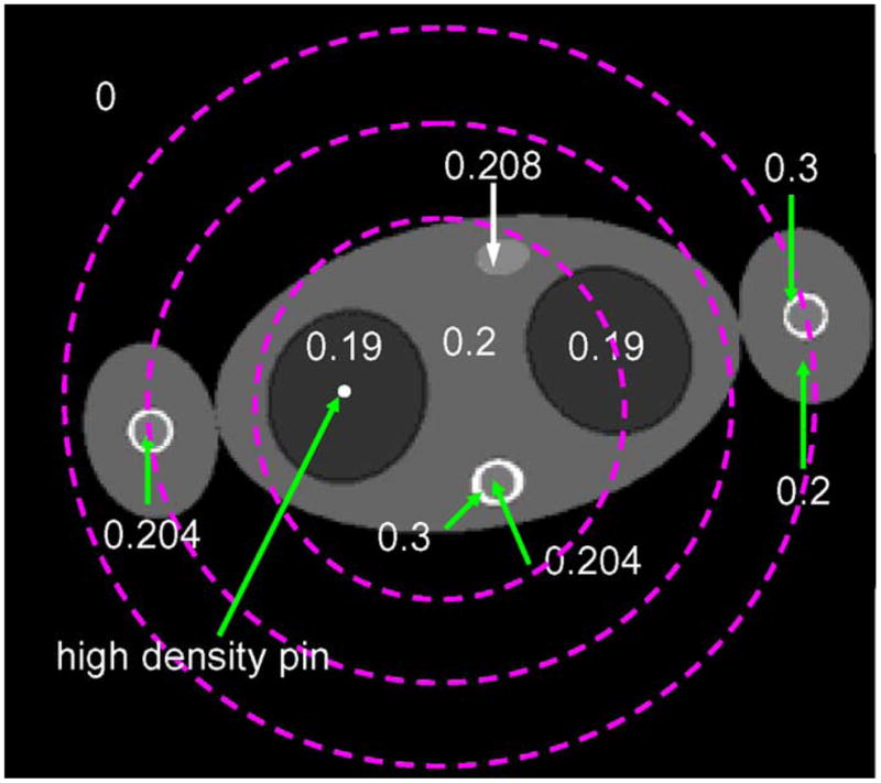
The phantom definition. The numbers indicate the attenuation values (cm−1) in different organs. The long axis of the body ellipse is 30 cm. This phantom is placed at (2.5, 2.5) cm from the iso-center. The dashed circles mark the SFOV at three truncation levels.
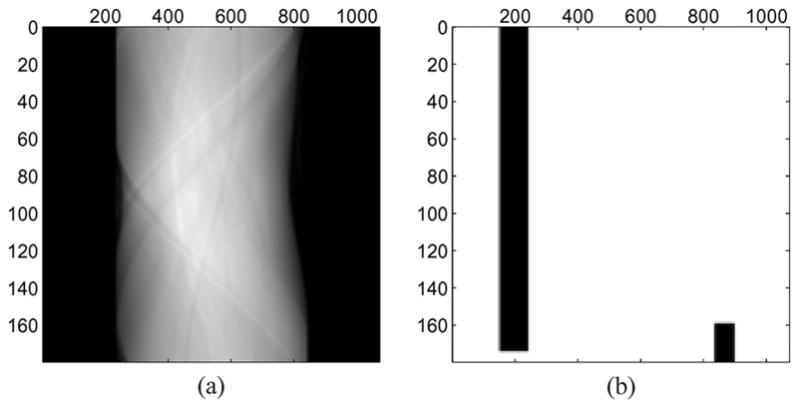
Fig. 3.
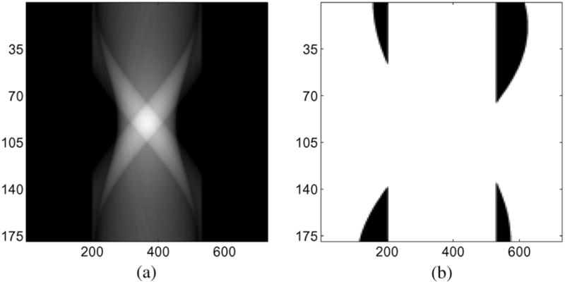
(a) The truncated projection data (after log operation). The vertical axis is the acquisition angle in degrees, the horizontal axis is the channel index. (b) The corresponding map of
(dark) and
(white). The cutoff channel number is t = 200 (FOV = 32.1 cm) in this example.
A. Dependence on the Degree of Data Truncation
At each air scan intensity level 108, 107, and 106, we varied the number of cutoff channels t and compared the performance of our proposed sinogram completion method with the symmetric mirroring method [6]. The complete projection data consisted of 729 channels and 512 views over 180° acquisition. Fig. 3 shows one example of the truncated projection data (line integrals) at t = 200 (FOV = 32.1 cm) and the corresponding trust region map with
(dark) and
(white) derived from the exact object boundary.
Since our simulation was performed in the parallel geometry and data truncation was artificial, we skipped steps 1 and 2 in the flowchart of Section III-C. Both the truncated projection data [the scaled, exponentiated version of Fig. 3(a)] and the trust region map [Fig. 3(b)] went through cosine-transform along the channel direction, and followed the steps in the flowchart until the final reconstructed images were obtained. The implementation of symmetric mirroring method and the related parameter settings followed the description in [6]. For each truncation case t = 150 (SFOV = 42 cm) of t = 200 (SFOV = 32 cm), and t = 250 (SFOV = 22 cm), we plotted the mean profile, from 20 noise realizations at the air scan 108, across the long axis of the reconstructed images obtained from different methods.
B. Dependence on the Accuracy of the Object Support Estimate
We also studied the performance of our proposed method when different object support estimates were used. In addition to the exact object support (see also Fig. 3), we also used a tight convex object support, and a loose rectangle support estimate shown in Fig. 4. The object support estimate was forward projected to generate the trust region
and
. Similar to Section IV-A, we plotted the mean profile across the long axis over the reconstructed images using our proposed method but with different estimation of the trust region maps. We evaluated the reconstructed images within the SFOV and the extended RFOV separately.
Fig. 4.
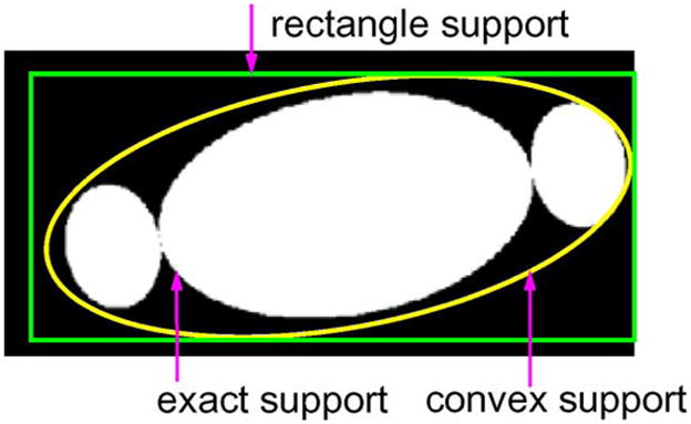
Three object support estimates: the exact object support, a tight convex support, and a loose rectangle object support.
C. Dependence on the Regularization Weight β and Different Statistical Assumptions
If we compare the problem formulation in (12) or (15) with the flowchart in Section III-C, we notice that the sinogram restoration algorithm is applied to the cosine-transformed projection data, not the projection data themselves. This can be considered a side effect of resorting to FFT for converting between l and the basis expansion coefficients b. The implementation in the flowchart however makes the sinogram restoration performance statistically suboptimal, for either the Poisson or the Gaussian model. To evaluate the noise properties of the proposed method, we use simulation studies to compare the noise-resolution tradeoffs of the two sinogram restoration methods with that of the symmetric mirroring method. A better solution is discussed at the end of the paper.
As the weighting factor β in (12) and (15) varies, the noise and resolution properties in the final FBP reconstructed image trace out a noise-resolution tradeoff curve. To calculate a resolution measure, we used zoomed FBP reconstruction from noise-free projection data (with the same truncation level t as the noisy projection data, and going through the same projection completion procedure). The resolution was then measured as the full-width-at-half-maximum of a 2-D Gaussian fitted to the image of the pin. The noise was calculated as the coefficient of variation (COV) in a nearby region-of-interest (ROI) of the pin location. For this study, we fixed the air scan intensity to be 106, and used the tight convex mask as the sinogram support. We varied the regularization weight β from 10−3 to103 and compared the noise-resolution tradeoff curves in the FBP reconstructed images using projection data obtained from (12) and (15), respectively. In the weighted least squares formulation, the pixel-dependent was taken to be 1/yi, the inverse of the transmission data. As a reference, we also plotted the tradeoff curve for the symmetric mirroring + FBP method. The reconstructed images were postsmoothed by Gaussian-shaped filters. The FWHM of the postsmoothing Gaussian filter serves the same purpose as β in the statistical formulations.
V. Computer Simulation Results
Shown in Figs. 5–10 are the results from the computer simulations. Fig. 5 is a plot of the objective function in (12) as a function of iteration numbers. We notice the monotonic increase of the objective function as the iteration continues. At the later iterations (≥ 50), the increase in the objective function per iteration is small compared with the earlier iterations. The complete sinogram takes more iterations to converge than the apparent plateau of the objective function. Fig. 6 shows some sample reconstruction images at different truncation levels using five different processing methods. The air scan intensity to produce the sample images is the lowest in our simulations at 106. Figs. 7–9 are the mean profiles of the five reconstruction methods at the truncation level of t = 150, 200, and 250, respectively. Fig. 10 compares the noise-resolution tradeoff of two statistical sinogram restoration methods with that of the symmetric mirroring method. The simulated air scan intensity is 106 and the truncation level t = 200.
Fig. 5.
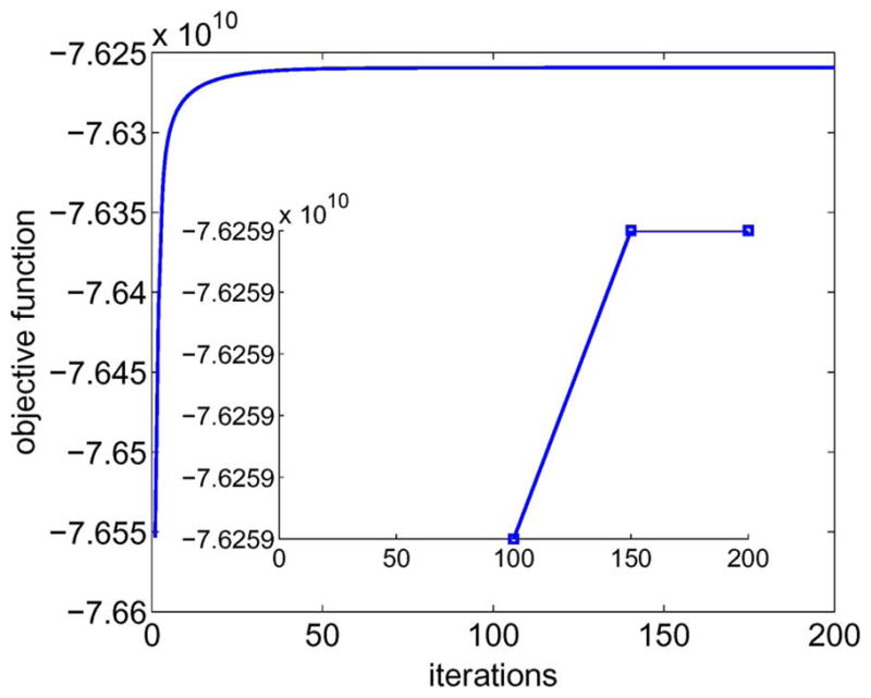
A sample objective function plot of the formulation (12) for the case of t = 200 and air scan level 106. The inlet zoomed in on the change in the objective function at later iterations. The objective function increase is small compared to the objective function value itself, i.e., smaller than 1e-5. This explains the vertical axis labels of the inlet.
Fig. 10.
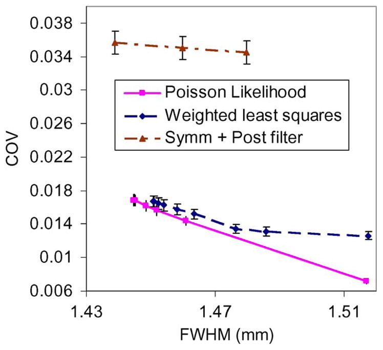
The noise-resolution tradeoffs at the pin location.
Fig. 6.

Results of the computer simulation study. The different columns correspond to different number t of truncated channels, and different rows different processing methods. 1st row: no correction. 2nd row: symmetric mirroring. 3rd–5th rows: our proposed method (12) with different support estimates. The air scan intensity to produce these sample images is 106. The display window for all images is [0.15, 0.25] cm−1.
Fig. 7.

The mean profile calculated from 20 noise realizations at t = 150 near the edge of data truncation (right side of SFOV). The black arrow points to the edge of data truncation.
Fig. 9.

Similar to Fig. 8 but at t = 250.
A. Sample Reconstruction Images
From Fig. 6 we observe that when the truncated projection data are directly applied to the FBP algorithm, the reconstructed images show significant positive bias, the bright band artifacts, near the edge of the SFOV. This bias is greatly reduced by applying either the symmetric mirroring method or our proposed sinogram restoration method. Using our proposed method, some remaining truncation artifacts can still be seen in the most severe truncation case t = 250 (Fig. 6, red arrows). The differences between the different support estimates mainly show up outside the SFOV. The exact support estimate helps to delineate the object boundary (Fig. 6, green arrows).
B. Dependence on the Degree of Data Truncation
From the mean profile plots (Figs. 7–9), we notice that within the SFOV our proposed method using any of the three object support estimates has smaller bias than the symmetric mirroring method. The same observation is made at the three different truncation levels. Unlike the symmetric mirroring method which uses ad-hoc data extrapolation, the proposed method uses the HL condition and tries to estimate the sinogram based on the available data and prior object support information. It is expected that the proposed method should provide more accurate reconstruction within the SFOV.
For the most severe truncation case (t = 250), some remaining edge artifacts (profile discontinuity) can be seen using the proposed method (Fig. 9(a) and (b), black arrows), while there is smaller discontinuity around the edges using the symmetric mirroring method. This observation agrees with the visual impression from Fig. 6 (third column, red arrows). For the other two truncation cases (t = 150, 200), the proposed method with the exact object support estimate has smaller errors than the symmetric mirroring at the edge of truncation in Fig. 7 and Fig. 8(a), and comparable errors with symmetric mirroring in Fig. 8(b). It appears that the remaining edge artifact using our proposed method is related to the truncation level in the available data. We have used the same parameter settings (stopping criterion and the smoothing parameter β) to produce all the reconstruction results. Finer parameter tuning in our proposed method should be examined.
Fig. 8.

Similar to Fig. 7 but at t = 200. Since both sides of the phantom are truncated, we use two arrowheads to indicate the edges of data truncation. (a) and (b) are near the left and right side of the SFOV in the region near data truncation.
C. Dependence on the Accuracy of the Object Support Estimate
The results from the different object support estimates do not differ much within the SFOV, except when the truncation is severe (t = 250) the results from the loose rectangle support show larger bias [Fig. 9(b)] than the exact object support and the tight convex support.
The advantage of using the exact object support is mainly in the extended RFOV (Fig. 6, green arrows). There is a gradual improvement in object boundary delineation when the sinogram restoration is applied with the loose rectangle support estimate, the convex support estimate, and the exact support; and all three have smaller mean profile error than the symmetric mirroring method. The reconstructed object boundary in the symmetric mirroring method is determined indirectly from the number of extended channels Next [6], an input parameter based on subjective judgment. On the other hand, the object support estimate enters our proposed method as part of the problem formulation. The reconstruction results are then more intuitive; the better the object support estimate is, the better delineation of the object boundary can be obtained.
D. Dependence on the Regularization Weight β and Different Statistical Assumptions
Fig. 10 shows the noise-resolution tradeoff curves in the FBP reconstructed images after projection completion using the symmetric mirroring method, the Poisson assumption (12), and the weighted least squares formulation (15). Compared with the analytic formulation, i.e., the symmetric mirroring method, there is a significant improvement in terms of noise resolution tradeoff using either of the statistical formulations. The Poisson assumption performs marginally better than the weighted least squares model at the simulated noise level.
We do notice that for the two sinogram restoration methods, the variation in the final (rather large) FWHM is relatively small despite change in β from 10−3 to 103. Two possible causes may play a role here. The effect of β is related to its relative magnitude with respect to the air scan (106) and the object attenuation properties (attenuation line integrals from 0–9). For paths through the object that are not severely attenuated, the relative magnitude of β is small. The rather large FWHM could be attributed to the channel-wise cosine and arc-cosine interpolation in the sinogram restoration procedure (cf. flowchart in Section III). Note that these interpolations are performed only once at the beginning and the end of the sinogram restoration procedure, not repeatedly at each iteration.
VI. Patient Data
We studied the performance of the proposed method using a data set from an obese patient whose body size extended outside of the SFOV. The original fan-beam projection has 672 (channels) × 1052 (views) per 360° acquisition covering a SFOV of 50 cm diameter. We compared three processing methods: 1) direct FBP of the truncated projection data, 2) FBP after projection completion using the symmetric mirroring method, and 3) after applying our proposed method.
The symmetric mirroring method was performed in the native fan beam geometry and fan beam FBP reconstruction was applied afterwards. To apply our proposed sinogram completion algorithm, we performed fan to parallel rebinning with interpolation; the rebinned parallel data has 673 channels and 1024 views per 180° acquisition. We padded 200 zero channels on either end of the rebinned parallel data to extend the FOV to 79.7 cm [Fig. 11(a)]. From the truncated projection data in Fig. 11(a), we obtained the trust region map of Fig. 11(b) by visually identifying those truncated channels and marked them off as banded
. The left band has a width of 90 channels, and the right band 60 channels. The two numbers are chosen purely based on visual judgment. Using the trust region map of Fig. 11(b), the sinogram completion algorithm then further confines the patient size to be 823(= 90+60+673) channels or 61 cm. Since the raw data were (scaled) line-integrals (after log-operation), we exponentiated the line-integrals and then scaled them by an arbitrary air scan intensity3 of 106. Similar to the processing of the simulation data, the (exponentiated) truncated projection and the trust region map were processed following the steps in the flow chart of Section III-C until the final reconstructed images were obtained.
Fig. 11.
(a) Truncated projection data (line-integrals) of the patient scan after fan beam to parallel beam rebinning. The horizontal axis is the channel index, the vertical axis is the acquisition angle in degrees. (b) The trust region map showing
(dark) and
(white) for the patient data.
Fig. 12 shows the reconstructed images from the three processing methods. To obtain a quantitative measure, we calculate the mean attenuation value within the three ROI’s (Fig. 12(a), green regions) located inside the SFOV. The middle ROI is far from the truncation artifacts, therefore is used a reference for calculating the percent bias within ROI-1 and ROI-2 that are near the truncation artifacts. The bias values are charted in Fig. 12(d). Using either the symmetric mirroring method or the proposed sinogram completion method, the bright boundary artifacts and the positive bias in the peripheral region within the SFOV are significantly reduced. The proposed method produces smaller bias than the symmetric mirroring method.
Fig. 12.
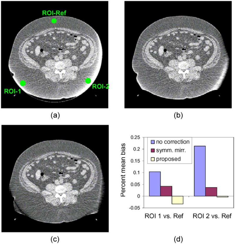
Reconstructed images (a) without correction, (b) with symmetric mirroring method, and (c) with our proposed method. (d) Comparison of percent bias. The display window is [0.14, 0.21] cm−1.
VII. Discussion and Conclusion
There are two main ideas we would like to convey in this paper. The first is that the consistency conditions can be incorporated in a sinogram restoration algorithm for transmission X-ray CT to accommodate projection data incompleteness. The second is that such an algorithm can be implemented in a simple, efficient, and numerically stable manner.
In our simulation studies, we used the parallel beam geometry and generated Poisson distributed transmission CT data and applied the algorithms in Section III. By varying the number of truncated channels, we studied the performance of the algorithm at different levels of data truncation. We also compared the noise-resolution tradeoff in the final FBP reconstructed images using the proposed method with the symmetric mirroring method. The proposed sinogram restoration approach greatly improved both the accuracy and the precision of the reconstructed images within the SFOV. The trust region map or the object support estimate does not affect the reconstructed images within the SFOV significantly, however a more accurate object support estimate can better delineate the object boundary in the extended RFOV. The three object support estimates that we have in Fig. 4 are all reasonably accurate. In a real imaging environment, some a priori knowledge of the object size may be necessary to obtain the sinogram support estimate. We point out that this is not an extra requirement for applying our method. Some knowledge of object size is needed for other truncation artifacts reduction algorithms as well, e.g., the zero-padding part for the symmetric mirroring method. Even in a fully iterative image reconstruction method, a prerequisite for the iteration to handle truncation “naturally” is to have a reconstruction matrix large enough to fully contain the object. If the object size is under estimated, then artifacts will occur at the edge of the SFOV and the prescribed RFOV.
At the three simulated data truncation levels (t = 150, 200, and 250), not all projection views are truncated. Analytical reconstruction algorithms have been developed [26] and [27] to produce exact reconstruction in the region where the SFOV intersects with the object. A crucial element in these theoretical developments is the use of object space information such as object support. The proposed sinogram restoration approach works exclusively in the sinogram domain. Though a priori sinogram domain knowledge can be incorporated, we do recognize that the sinogram domain constraints (e.g., sinogram support) can be much weaker than the object space constraints (e.g., object support). Therefore we must caution that theoretical exactness (zero bias) using the proposed sinogram restoration method may not be guaranteed; this is in addition to the bias introduced through the regularization factor β. However, a marked difference from the approaches in [26], [27] is that we also seek to recover beyond the SFOV. Our computer simulations obtained not only excellent results within the SFOV, but made regions beyond the SFOV visible. Moreover, the statistical formulation makes our approach less prone to data noise, a common weakness of many analytical reconstruction algorithms.
We also applied our projection completion algorithm to real patient data. The positive bias in the peripheral regions of the patient was greatly reduced, but within the extended RFOV the object boundary was not as well recovered as in the simulation studies. Since the acquired raw patient data were scaled line-integrals, we needed to exponentiate the patient data first to obtain the transmission CT data. An arbitrary, constant air scan intensity was used since the relevant information was unavailable to us. This approach has been used in other works though its validity might be arguable. In a clinical CT scanner, the application of bow-tie filters results in a nonconstant air scan intensity profile. The mismatch between this and our assumed constant air scan intensity may quantitatively affect the noise properties of the final reconstructed image. A better way may be to estimate the air scan intensity from the variance of the blank scan (no object) projection values [25], [28], and use the estimated air scan instead of an arbitrary constant to scale the exponentiated line integrals.
For the iterative algorithm that we proposed, the computational efficiency depends on 1) the number of iterations and 2) the computations per iteration. In terms of iteration numbers, the sinogram restoration algorithm now on the average runs to ~1000 iterations. It is often found that fully iterative algorithms run to thousands of iterations (counting subset updates) [29], [30]. The computational advantage of the proposed method mainly comes from the application of the FFT instead of the regular forward/backward projection operators. The paper [31] demonstrated the computational savings of using FFT method for forward/backward projector calculations. For typical image size, [31] showed more than 50% computational savings; and this advantage increases with image size.
There are some unaddressed questions in this paper. Our evaluation studies are still preliminary. We have not performed quantitative comparisons with other projection completion algorithms such as [5] and [9], nor have we studied the role and effect of the smoothing parameter β. In principle, both the HL consistency condition (by its finite number of bkm terms) and the quadratic penalty R regulate the solution. For the results reported in this paper, the number of the expansion terms bkm was simply determined from the channel numbers and the view numbers. It is interesting to investigate the interplay between the parameter β and the Fourier transform length (# of bkms) and their effects on the final reconstructed images. Further research may also look into how the completed sinograms, hence the reconstructed images from them, evolve as a function of iteration numbers.
If the phantom simulations were performed in the native fan beam geometry, the interpolation from fan beam to parallel beam geometry will change the probability distribution of the rebinned data, and invalidate the assumption that the rebinned data are Poisson distributed random variables. We may alternatively construct the following function:
| (16) |
The unknowns l are defined on a parallel beam grid, and the measurements yi, i ∈
are defined on the native fan beam grid. Here {aij > 0} may be regarded as a rebinning matrix that takes care of the parallel to fan rebinning. The optimization problem is then to maximize the objective function in (16) subject to the constraint that l satisfies the HL condition. It will be interesting to compare this alternative model with our approach presented here in terms of image noise and resolution.
There are other possible extensions of this work. Since our problem formulation is completely general, the projection incompleteness is not confined to channel-wise data truncation, though these are the cases we studied in the simulation and experiments. Other types of data incompleteness, such as limited angle data acquisition and sparse sampling are also interesting application areas of our proposed method.
Acknowledgments
This work was supported in part by a research contract with Siemens Healthcare.
The authors would like to thank E. Fishman, M.D., B. Mudge, and E. Avril for their assistance with patient data acquisition. The authors would also like to thank K. Stierstorfer, Ph.D. at Siemens Healthcare for his help with Siemens scanner data format.
Appendix A Derivation of (14)
We denote by L the objective function in (12). Since for e−l ≤ 1 − l + l2 for l > −1.5, we have
It is straightforward to verify that L(l) ≥ Φ(l; l−) if l − l− > −1.5, and L(l−) = Φ(l−; l−). According to [21], Φ(l; l−) is a legitimate surrogate function of the objective function L of (12) if we restrict the step size of l such that l − l− > −1.5. By completion of squares, we can rewrite the surrogate function Φ(l; l−) in the following form:
where
N is the total number of neighborhood pixels (N =4 in this work), and
| (17) |
Now plugging in the constraint equation l = Qb with the understanding that only bf in are the effective unknowns, we seek b such that
| (18) |
is maximized. In (18) we define Λ(l−) = diag[λ1(l−), λ2(l−), ···], a diagonal matrix with the ith element λi(l−), i ∈
, and F(l−) a column vector with elements fi(l−), i ∈
. The following optimality condition of (18):
| (19) |
Suppose Λ(l−) = I is the identity operator, then the solution to (19) is simply b = [QT F(l−)]r by the orthogonality condition of the operator Q. In general, the solution of (19)
| (20a) |
| (20b) |
but the matrix inversion in (20b) may be costly to compute at each iteration. Instead we derive a second surrogate function of in Φ(l; l−) (18) to replace the diagonal matrix Λ(l−) by a scaled identity matrix. The derivation is based on the observation that, for D a diagonal positive definite matrix, D = diag[d1, d2, ···], and x an arbitrary real number
| (21) |
where dmin is the minimal diagonal element of D. From (21), it is easy to verify that dminxT x is a (trivial) surrogate (at the point x = 0) for minimizing xT Dx. We use the same trick to rewrite Φ(l; l−) as follows:
| (22) |
| (23) |
where λmin = miniλi(l−), i ∈
, λmin < 0. The inequality in (23) defines a second surrogate function of Φ(l; l−) whose solution is
| (24) |
The above derivation requires that the change in l is bounded from below by −1.5. Since l = Qb, we have ||δl|| ≤ ||Q|| ||δb||. With proper normalization of Q, QTQ = I, the maximum change in l can be verified and ensured by the maximum change in b, which in turn, if necessary, can be adjusted by replacing the relaxation parameter 1/|λmin| in (24) by some 0 < α < 1/|λmin|, λmin < 0.
Appendix B Weighted Least Squares Projection Completion Algorithm
The algorithm derivation is analogous to the Poisson distribution case. Since the objective function in (15) is quadratic, we may skip the first quadratic surrogate function. By comparing terms, it is straightforward to verify that
The rest of the derivation is exactly the same as in Appendix A with the above λi(l−) and fi(l−) that define Λ(l−) and F(l−).
Footnotes
We abbreviate the Helgason-Ludwig consistency condition as the HL condition in the rest of the paper for convenience.
Here, “available” means either measured, or not measured but assumed to be zero, i.e., outside of the projection support region. See Section III-E.
Scaling by an arbitrary air scan intensity may cause statistical model mismatch. We address this problem further in Section VII.
Contributor Information
Jingyan Xu, Email: jxu@jhmi.edu, Division of Medical Imaging Physics, Department of Radiology, Johns Hopkins University School of Medicine, Baltimore, MD 21287 USA.
Katsuyuki Taguchi, Email: ktaguchi@jhmi.edu, Division of Medical Imaging Physics, Department of Radiology, Johns Hopkins University School of Medicine, Baltimore, MD 21287 USA.
Benjamin M. W. Tsui, Email: btsui1@jhmi.edu, Division of Medical Imaging Physics, Department of Radiology, Johns Hopkins University School of Medicine, Baltimore, MD 21287 USA
References
- 1.Herman GT, Lewitt RM. Evaluation of a preprocessing algorithm for truncated CT projections. J Comput Assist Tomogr. 1981 Feb;5(1):127–135. doi: 10.1097/00004728-198102000-00026. [DOI] [PubMed] [Google Scholar]
- 2.Lalush DS, Tsui BM. Performance of ordered-subset re-construction algorithms under conditions of extreme attenuation and truncation in myocardial SPECT. J Nucl Med. 2000 Apr;41(4):737–744. [PubMed] [Google Scholar]
- 3.Snyder DL, O’Sullivan JA, Murphy RJ, Politte DG, Whiting BR, Williamson JF. Image reconstruction for transmission tomography when projection data are incomplete. Phys Med Biol. 2006 Nov;51:5603–5619. doi: 10.1088/0031-9155/51/21/015. [DOI] [PubMed] [Google Scholar]
- 4.Manglos SH. Truncation artifact suppression in cone-beam radionuclide transmission CT using maximum likelihood techniques: Evaluation with human subjects. Phys Med Biol. 1992 Mar;37(3):549–562. doi: 10.1088/0031-9155/37/3/004. [DOI] [PubMed] [Google Scholar]
- 5.Hsieh J, Chao E, Thibault J, Grekowicz B, Horst A, McOlash S, Myers TJ. A novel reconstruction algorithm to extend the CT scan field-of-view. Med Phys. 2004;31(9):2385–2391. doi: 10.1118/1.1776673. [Online]. Available: http://link.aip.org/link/?MPH/31/2385/1. [DOI] [PubMed] [Google Scholar]
- 6.Ohnesorge B, Flohr T, Schwarz K, Heiken JP, Bae KT. Efficient correction for CT image artifacts caused by objects extending outside the scan field of view. Med Phys. 2000 Jan;27(1):39–46. doi: 10.1118/1.598855. [DOI] [PubMed] [Google Scholar]
- 7.Helgason S. The Radon transform on Euclidean spaces, compact two-point homogeneous spaces and Grassmann manifolds. Acta Mathematica. 1965 Jul;113(1):153–180. [Google Scholar]
- 8.Ludwig D. The Radon transform on Euclidean space. Commun Pure Appl Math. 1966;XIX:49–81. [Google Scholar]
- 9.Zamyatin AA, Nakanishi S. Extension of the reconstruction field of view and truncation correction using sinogram decomposition. Med Phys. 2007;34(5):1593–1604. doi: 10.1118/1.2721656. [Online]. Available: http://link.aip.org/link/?MPH/34/1593/1. [DOI] [PubMed] [Google Scholar]
- 10.Chityala R, Hoffman KR, Rudin S, Bednarek DR. Artifact reduction in truncated CT using sinogram completion. Proc SPIE Med Imag, Conf Image Process. 2005;5747:2110–2117. doi: 10.1117/12.595450. [DOI] [PMC free article] [PubMed] [Google Scholar]
- 11.Sourbelle K, Kachelriess M, Kalender WA. Reconstruction from truncated projections in CT using adaptive detruncation. Eur Radiol. 2005 May;15(5):1008–1014. doi: 10.1007/s00330-004-2621-9. [DOI] [PubMed] [Google Scholar]
- 12.Chen G-H, Leng S. A new data consistency condition for fan-beam projection data. Med Phys. 2005;32(4):961–967. doi: 10.1118/1.1861395. [Online]. Available: http://link.aip.org/link/?MPH/32/961/1. [DOI] [PubMed] [Google Scholar]
- 13.Kudo H, Saito T. Sinogram recovery with the method of convex projections for limited-data reconstruction in computed tomography. J Opt Soc Am, A. 1991 Jul;8(7):1148–1160. [Google Scholar]
- 14.Prince JL, Willsky AS. Constrained sinogram restoration for limited-angle tomography. Opt Eng. 1990 May;29(5):535–544. [Google Scholar]
- 15.Natterer F. The Mathematics of Computed Tomography. Philadelphia, PA: SIAM Classics in Applied Mathematics; 2001. [Google Scholar]
- 16.De Pierro AR. On the relation between the ISRA and the EM algorithm for positron emission tomography. IEEE Trans Med Imag. 1993 Jun;12(2):328–333. doi: 10.1109/42.232263. [DOI] [PubMed] [Google Scholar]
- 17.Lange K, Hunter DR, Yang I. Optimization transfer using surrogate objective functions. J Computat Graphical Stat. 2000 Mar;9(1):1–20. [Google Scholar]
- 18.Gentleman WM. Implementing Clenshaw-Curtis quadrature, II computing the cosine transformation. Commun ACM. 1972;15(5):343–346. [Google Scholar]
- 19.Bortfeld T, Oelfke U. Fast and exact 2-D image reconstruction by means of Chebyshev decomposition and backprojection. Phys Med Biol. 1999 Apr;44:1105–1120. doi: 10.1088/0031-9155/44/4/020. [DOI] [PubMed] [Google Scholar]
- 20.La Riviere PJ, Bian J, Vargas PA. Penalized-likelihood sinogram restoration for computed tomography. IEEE Trans Med Imag. 2006 Aug;25(8):1022–1036. doi: 10.1109/tmi.2006.875429. [DOI] [PubMed] [Google Scholar]
- 21.Erdogan H, Fessler JA. Monotonic algorithms for transmission tomography. IEEE Trans Med Imag. 1999 Sep;18(9):801–814. doi: 10.1109/42.802758. [DOI] [PubMed] [Google Scholar]
- 22.Erdogan H, Fessler JA. Ordered subsets algorithms for transmission tomography. Phys Med Biol. 1999;44(11):2835–2851. doi: 10.1088/0031-9155/44/11/311. [Online]. Available: http://stacks.iop.org/0031-9155/44/2835. [DOI] [PubMed] [Google Scholar]
- 23.Hsieh J. Computer Tomography, Principles, Design, Artifacts, and Recent Advances. 1. Bellingham, WA: SPIE; 2003. [Google Scholar]
- 24.Ziegler A, Köhler T, Proksa R. Noise and resolution in images reconstructed with FBP and OSC algorithms for CT. Med Phys. 2007;34(2):585–598. doi: 10.1118/1.2409481. [Online]. Available: http://link.aip.org/link/?MPH/34/585/1. [DOI] [PubMed] [Google Scholar]
- 25.Wang J, Lu H, Liang Z, Eremina D, Zhang G, Wang S, Chen J, Manzione J. An experimental study on the noise properties of X-ray CT sinogram data in Radon space. Phys Med Biol. 2008 Jun;53:3327–3341. doi: 10.1088/0031-9155/53/12/018. [DOI] [PMC free article] [PubMed] [Google Scholar]
- 26.Noo F, Clackdoyle R, Pack JD. A two-step Hilbert transform method for 2-D image reconstruction. Phys Med Biol. 2004 Sep;49:3903–3923. doi: 10.1088/0031-9155/49/17/006. [DOI] [PubMed] [Google Scholar]
- 27.Defrise M, Noo F, Clackdoyle R, Kudo H. Truncated Hilbert transform and image reconstruction from limited tomographic data. Inverse Problems. 2006 Jun;22:1037–1053. [Google Scholar]
- 28.Whiting BR, Massoumzadeh P, Earl OA, O’Sullivan JA, Snyder DL, Williamson JF. Properties of preprocessed sinogram data in X-ray computed tomography. Med Phys. 2006;33(9):3290–3303. doi: 10.1118/1.2230762. [Online]. Available: http://link.aip.org/link/?MPH/33/3290/1. [DOI] [PubMed] [Google Scholar]
- 29.Man BD, Nuyts J, Dupont P, Marchal G, Suetens P. An iterative maximum-likelihood polychromatic algorithm for CT. IEEE Trans Med Imag. 2001 Oct;20(10):999–1008. doi: 10.1109/42.959297. [DOI] [PubMed] [Google Scholar]
- 30.O’Sullivan J, Benac J. Alternating minimization algorithms for transmission tomography. IEEE Trans Med Imag. 2007 Mar;26(3):283–297. doi: 10.1109/TMI.2006.886806. [DOI] [PubMed] [Google Scholar]
- 31.O’Connor Y, Fessler J. Fourier-based forward and back-projectors in iterative fan-beam tomographic image reconstruction. IEEE Trans Med Imag. 2006 May;25(5):582–589. doi: 10.1109/TMI.2006.872139. [DOI] [PubMed] [Google Scholar]