Abstract
One of the most popular paradigms to use for studying human reasoning involves the Wason card selection task. In this task, the participant is presented with four cards and a conditional rule (e.g., “If there is an A on one side of the card, there is always a 2 on the other side”). Participants are asked which cards should be turned to verify whether or not the rule holds. In this simple task, participants consistently provide answers that are incorrect according to formal logic. To account for these errors, several models have been proposed, one of the most prominent being the information gain model (Oaksford & Chater, Psychological Review, 101, 608–631, 1994). This model is based on the assumption that people independently select cards based on the expected information gain of turning a particular card. In this article, we present two estimation methods to fit the information gain model: a maximum likelihood procedure (programmed in R) and a Bayesian procedure (programmed in WinBUGS). We compare the two procedures and illustrate the flexibility of the Bayesian hierarchical procedure by applying it to data from a meta-analysis of the Wason task (Oaksford & Chater, Psychological Review, 101, 608–631, 1994). We also show that the goodness of fit of the information gain model can be assessed by inspecting the posterior predictives of the model. These Bayesian procedures make it easy to apply the information gain model to empirical data. Supplemental materials may be downloaded along with this article from www.springerlink.com.
Electronic supplementary material
The online version of this article (doi:10.3758/s13428-010-0057-5) contains supplementary material, which is available to authorized users.
Keywords: Wason card selection task, Optimal data selection, Probabilistic reasoning, Bayesian parameter estimation, Maximum likelihood estimation
The Wason card selection task (Wason, 1966) has become a classic task in research on human reasoning (Evans & Over, 2004; Oberauer, Wilhelm, & Diaz, 1999; Stenning & van Lambalgen, 2008). The Wason task was originally designed to highlight the tendency of people to search for confirmatory evidence and ignore potentially falsifying evidence. In the most common version of the Wason task, the participant is shown four cards; each card has a letter on one side and a number on the other. Two cards have the letter side facing upward, and two cards have the number side facing upward—for example, A, K, 2, 7. The participant is then presented with a conditional rule such as “If there is an A on one side of the card, there is always a 2 on the other side.” Participants must determine which cards they need to turn in order to verify whether or not this conditional rule holds.
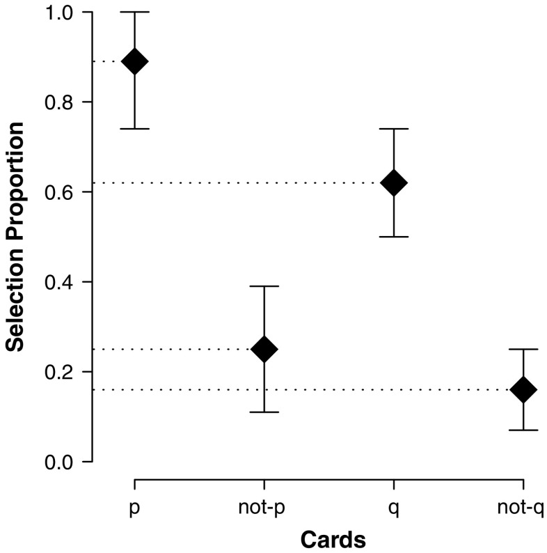
The antecedent of the rule (in this example, the A card) is generally called p, and the consequence of the rule (in this example, the 2 card) is called q. Figure 1 shows the selection probabilities of the four cards in the Wason task from a meta-analysis by Oaksford and Chater (1994). This analysis confirms that most people turn the p card and the q card (Oaksford & Chater, 1994). Turning the q card confirms the rule if a p is found on the other side. This confirmatory strategy is not logically sound, though. Finding example cards that correspond to the rule does not prove the rule to be generally true. Propositional logic dictates that the not-q card (in this case, the 7 card) should be turned instead of the q card. To see this, note that the only violation of the rule is a (p, not-q) card. So, to falsify the rule, it is necessary to turn both the p card and the not-q card.
Fig. 1.
Typical choice behavior in the Wason card selection task. Participants most often select the p and q cards, whereas formal logic dictates that the only correct selections are the p and not-q cards. Error bars indicate one standard deviation from the mean. Data are based on a meta-analysis reported by Oaksford and Chater (1994). See the text for details
Two types of explanations for this confirmatory bias can be distinguished (Klauer, Stahl, & Erdfelder, 2007).1 On the one hand, heuristic models claim that the variation in card selections is caused by different interpretations of the conditional rule. For example, if the rule is accidentally interpreted as bidirectional, both p and q need to be turned, the answer pattern that is chosen most frequently. Probabilistic models, on the other hand, assume that people select each card independently with a certain probability.
The most prominent probabilistic model of the Wason task is the information gain model (Oaksford & Chater, 2003). This model is a Bayesian model in the sense that it produces card selections that are rational and optimal given the available information and background knowledge. Although the information gain model itself is Bayesian, Oaksford and Chater (2003) used a maximum likelihood procedure to estimate the model’s parameters. This means that a rational model for human reasoning makes contact with the data in a nonrational manner. Thus, the participant in the Wason task is assumed to draw coherent and optimal conclusions from uncertain information, but the researcher who analyzes the data is satisfied with conclusions that are incoherent and suboptimal (Kruschke, 2010).
The goal of this article is to resolve this paradoxical tension between models for human reasoning and models for statistical inference by providing researchers with an easy-to-use Bayesian fitting routine for the information gain model.
Our Bayesian fitting routines use WinBUGS,2 a general-purpose program for implementing Bayesian models (Lunn, Spiegelhalter, Thomas, & Best, 2009; Lunn, Thomas, Best, & Spiegelhalter, 2000). We compare estimators from a nonhierarchical and a hierarchical Bayesian model with a maximum likelihood estimation procedure implemented in R.3 All three methods are illustrated with data from a meta-analysis by Oaksford and Chater (1994). We also show how the goodness of fit of the Bayesian information gain models can be assessed by inspecting the posterior predictives for card selection probabilities. All WinBUGS and R code is available from the the Psychonomic Society supplemental archive, as well as from the first author’s website.4
The information gain model
The information gain model is Bayesian and provides a probabilistic, rational explanation for why participants tend to select the logically incorrect p and q cards in the Wason task (Chater & Oaksford, 1999; Hattori, 1999, 2002; Klauer, 1999; Klauer, Stahl, & Erdfelder, 2007; Oaksford & Chater, 1994, 2001, 2003; Oberauer, Wilhelm, & Diaz, 1999). The model was motivated by the theory of optimal experimental design (e.g., Cavagnaro, Myung, Pitt, & Kujala, 2010; Cavagnaro, Pitt, & Myung, in press; Lindley, 1972; for a discussion, see Klauer, 1999), and its basic principles generalize to several other paradigms in human reasoning research that emphasize probability and rationality (Nelson, 2005; Oaksford & Chater, 2007).
A fundamental assumption in the information gain model is that people, when faced with the Wason task, pit two models against each other: an independence model and a dependence model. A priori, each model is assumed to be equally likely. The independence model assumes that the two sides of the cards are unrelated. In contrast, the dependence model assumes that cards conform to the conditional rule. However, the dependence model does involve an exception parameter ε that represents the probability of the rule occasionally failing. This parameter is typically set at .1, allowing for a 10% exception rate (Oaksford & Chater, 2003). This parameter is fixed in order to limit the number of free parameters.
The dependence and independence models predict different probabilities of finding a particular symbol (p or not-p and q or not-q, respectively) on the other side of a card. Although no cards are actually turned in the Wason task, the expected information gain of turning a particular card can be calculated. The selection probabilities of the cards are proportional to the expected information gain. Appendix A contains the mathematical details of the information gain model as discussed in Oaksford and Chater (2003).
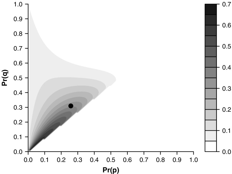
The information gain model contains two free parameters: a and b, which are the prior probabilities of a p or q symbol on a card. If these probabilities are relatively low, the model predicts that people will select the p and q cards instead of the logically correct p and not-q cards. Figure 2 shows the probabilities of selecting the p and q cards as a function of the prior probabilities a and b. The selection probabilities for cards p and q are high when prior probabilities a and b are low. The assumption that the prior probabilities for p and q are low is called the rarity assumption (Oaksford & Chater, 2003), an assumption that is based on the notion that in a world with many objects, the probability of encountering a particular object is relatively low.
Fig. 2.
Predictions from the information gain model for the probability of selecting both the p and q cards as a function of prior probabilities Pr(p) and Pr(q). The rarity assumption [i.e., low prior probabilities for Pr(p) and Pr(q)] results in a high probability of selecting cards p and q. The black dot indicates the ML estimate of the prior probabilities based on data from a meta-analysis reported by Oaksford and Chater (1994)
When the rarity assumption holds, the information gain model provides a rational explanation for why people tend to select cards that should not be selected according to propositional logic. Thus, the information gain model shows that people’s choice behavior in the Wason task may not come about because of inherent cognitive limitations and an unhealthy bias for confirmatory evidence; instead, the model shows that people may behave adaptively in an uncertain world. Note that the same results can be interpreted completely differently, depending on whether one uses propositional logic (e.g., “people make logically incorrect decisions and search primarily for confirmatory evidence”) or Bayesian reasoning (e.g., “people respond optimally given uncertain information”).
Parameter estimation
In the information gain model, only a and b, the respective prior probabilities of p and q, need to be estimated. The third parameter, ε—the exception parameter—is fixed to .1 (Oaksford & Chater, 2003). It is important to note that a and b are not independent in the information gain model. Under the dependence assumption, b cannot be much smaller than a, due to the 90% probability that q is on the other side of a p side. Since a = Pr(p) and b = Pr(q), it is evident that given this rule, b is restricted by a. To be precise, b > a(1 – ε). A convenient way to circumvent this problem is to reparameterize b as c using  , as suggested by Klauer et al. (2007). This reparameterization ensures that c can vary freely between zero and one, irrespective of a. The estimate of b can be now be computed deterministically from the estimates of a and c.
Maximum likelihood estimation
Parameters can be estimated in different ways. A popular method is maximum likelihood estimation (MLE; Myung, 2003), which provides the parameter values that maximize the probability of the observed data:  . The probability of the data given the parameter values are computed from the selection probabilities of the model (see Appendix A).
MLE has several attractive properties. First of all, it is asymptotically unbiased, meaning that for large samples, the bias approaches zero. MLE is also efficient, meaning that it asymptotically has the lowest mean squared error of all unbiased estimators. Furthermore, it can be shown that the MLE is also asymptotically better than any regular biased estimator (van der Vaart, 1998). There are several ways to obtain confidence intervals for the MLE. One option is bootstrapping (Efron & Tibshirani, 1993). In bootstrapping, the estimation procedure is repeated many times on randomly selected samples from the data, drawn with replacement. These repeatedly calculated measures can then be used to compute a bootstrap confidence interval. Alternatively, one could compute the square roots of the diagonals of the inverted negative Hessian in order to obtain standard errors for the MLE.
One of the limitations of MLE is that it is sensitive to local optima. One solution to this problem is to use a grid of initial values, a technique that works well for parameter spaces that are fairly regular. Each initial value is a different starting point in the parameter space that can result in a different local optimum. By using the estimate with the highest maximum, incidental local optima can be avoided. Of course, there is no guarantee that the global maximum will be found. However, for fine grids and regular parameter spaces, this should not be a problem in practice.
Bayesian estimation
An alternative estimation method is Bayesian. In Bayesian inference, uncertainty with respect to parameters is—at any point in time—quantified by probability distributions. This means that a distribution needs to be specified for all parameters in advance. These prior distributions reflect the a priori expectations with respect to the parameter values. Using Bayes’s rule to update the distribution of parameters a and c based on data D, we obtain posterior probability  , where C is a normalizing constant. Since a and c are assumed to be independent, the posterior can be rewritten as
  . Prior distributions p(a) and p(c) reflect any prior knowledge about the parameters. The likelihood p(D | a, c) is the probability of the observed data given a and c. The posterior distribution p(a, c | D) expresses our uncertainty with respect to the parameters of interest after seeing the data. Confidence intervals can be easily calculated from the posterior distribution, and the maximum a posteriori estimator (i.e., MAP; the mode of the posterior) provides point estimates. For uniform priors, MAP estimators equal ML estimators.
Bayesian models provide another advantage. It is relatively easy to extend Bayesian models in order to accommodate different levels of analysis. In the standard information gain model, trials in the Wason task are all assumed to be independent. In a meta-analysis, this is often not a valid assumption. A meta-analysis of different experiments introduces two levels of analysis: an experiment level and a trial level. Trials are only independent conditional on a participant. Hierarchical models are a natural solution for analyzing such multilevel data in a single model, since they explicitly account for conditional independences present in the hierarchical structure (Lee, in press). We have implemented both a nonhierarchical and a hierarchical Bayesian estimation procedure for the information gain model.
Although in some cases closed-form expressions of the posterior distribution exist, this is often not the case. Fortunately, it is now possible to approximate these distributions numerically using Markov chain Monte Carlo methods (MCMC; e.g., Gamerman & Lopes, 2006; Gilks, Richardson, & Spiegelhalter, 1996). With MCMC techniques such as Gibbs sampling or the Metropolis–Hastings algorithm, researchers can now directly sample sequences of values from the posterior distribution of interest, foregoing the need for closed-form analytic solutions.
Implementation of Bayesian models
Hand-coding MCMC algorithms can be effortful and error-prone, and the end result may be difficult for other researchers to understand or adjust. Therefore, we use the general-purpose WinBUGS program, which allows the user to specify and fit Bayesian models without having to hand-code the MCMC algorithms (Lunn et al., 2009; Lunn et al., 2000; an introduction for psychologists is given by Lee & Wagenmakers, 2010, Sheu & O’Curry, 1998; Wetzels, Lee, & Wagenmakers, 2010, discuss how to implement user-defined functions in WinBUGS). Although WinBUGS is flexible, it is not guaranteed to work for every application; problems with convergence may arise when the model is grossly misspecified or relatively complicated (e.g., mixture models with crossed random effects), especially when the data are relatively sparse. Nevertheless, WinBUGS will work for most applications in the field of psychology.
WinBUGS requires the user to provide a model specification, initial values for the model parameters, and of course the data. To implement the information gain model, we specified (1) a uniform prior distribution for parameters a and c, (2) a binomial distribution on all four card selection frequencies, with the respective card selection probabilities and sample size as parameters, and (3) a deterministic relation between the parameters a and c and the four card selection probabilities specified by the model. In this article, we present a nonhierarchical and a hierarchical Bayesian version of the information gain model.
The model specification can be represented graphically so as to facilitate understanding and communication (see Gilks, Thomas, & Spiegelhalter, 1994, for more information on graphical modeling). A graphical model consists of nodes connected with unidirectional arrows. Each node represents a probabilistic variable, whose distribution depends on the values of the parent nodes. These parent–child relations define all conditional and joint probabilities in the model and can be used to compute the posterior distribution.
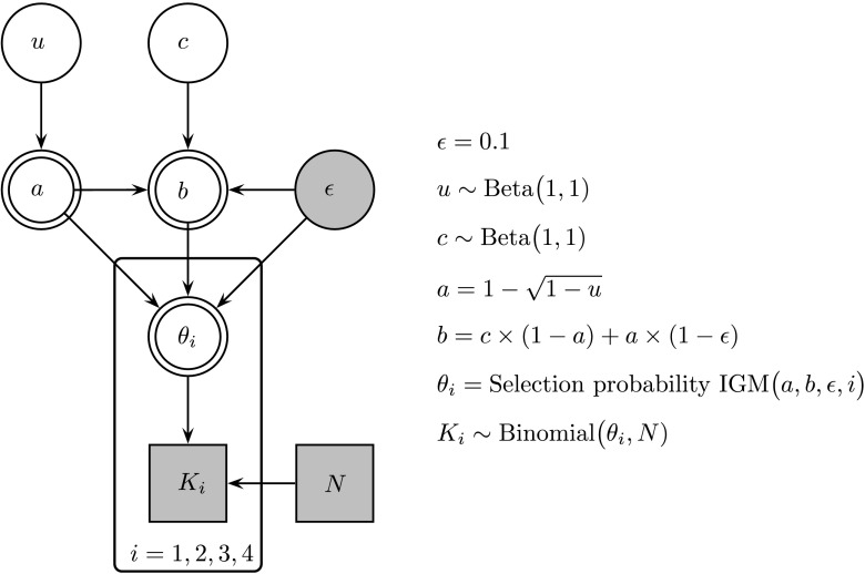
A graphical representation of the nonhierarchical information gain model is shown in Fig. 3. Circles reflect continuous variables, whereas boxes reflect discrete variables. The gray boxes are the observed number of trials (N) and the number of trials in which card i was selected (K i). The plate around θ i and K i denotes that the structure is repeated for each card i. K i is drawn from a binomial distribution with probability θ i and sample size N. The double circles around θ i indicate that this is a deterministic latent variable whose value is computed from parameters a, b, and fixed error ε (see Appendix A). Parameter c is a reparameterization of b with range [0, 1]. Unlike the uniform prior on c, the prior on a is a function of a uniformly distributed variable u. These priors ensure that the prior in (a, b) space is uniform instead of being heavily skewed due to the dependency between a and b (see Appendix B for details). This graphical model with corresponding distributions and deterministic relations fully defines the information gain model and can be used to estimate the posterior distribution of parameters a and b.
Fig. 3.
Graphical representation of the nonhierarchical information gain model implemented in WinBUGS. See the text for details
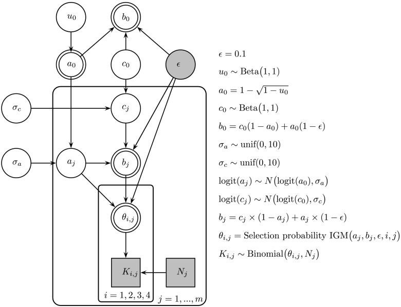
In a Bayesian framework, it is relatively easy to create a hierarchical extension of the information gain model (Fig. 4). Parameters a and c are now indexed, and each pair (a j, c j) refers to a different experiment. Instead of assigning priors directly to the experimental parameters, we now transform a and c to an unbounded scale using the logit function. The two transformed values are assumed to be drawn from a normal distribution, each with its own mean and variance. Since these intermediate means are defined on a unbounded scale, they are transformed back using the inverse logit function to obtain the population parameters a 0 and c 0, both of which lie between 0 and 1. It is on these population parameters that the priors are defined in a manner analogous to the nonhierarchical model. Again, b 0 can be computed from a 0 and c 0. This model allows for estimation of a and b both for the population (a 0 and b 0) and for each experiment or condition (a j and b j).
Fig. 4.
Graphical representation of the hierarchical information gain model implemented in WinBUGS. See the text for details
Estimation procedure
In this section, we discuss the estimation procedures for nonhierarchical Bayesian estimation, maximum likelihood estimation, and hierarchical Bayesian estimation. Nonhierarchical Bayesian estimation is compared with maximum likelihood estimation at the end of the section. These procedures require R, WinBUGS, the R package R2WinBUGS, and the code we have provided online.
Bayesian estimation
To allow users with no experience with WinBUGS to estimate the information gain model, we have created a function in R dealing with the WinBUGS calls.

The variable  should be a vector of length 4 with the number of trials that each card was selected. The order of the cards is expected to be (p, not-p, q, not-q). The variable
  is the total number of trials. Each trial consists of doing the Wason task once. The current model does not distinguish between trials of the same subject and trials of different subjects. Variable
  is the error probability that the conditional rule does not hold in the dependence model, which defaults to 10%.
MCMC algorithms require long chains of iterations to obtain reliable posterior distributions of the parameters. Variable  indicates how many iterations are computed per chain. WinBUGS uses several chains starting from different initial values. Because the first iterations of each chain are not yet converged to the true solution, they should be discarded. The
  variable indicates how many iterations should be discarded.
Convergence of the estimation procedure can be checked by visually inspecting whether the chains mix appropriately. Mixed chains increase confidence that the estimations are insensitive to particular initial values. The variable  is the number of chains used. The default value of 3 should be sufficient for visual inspection. The samples from the chains form a histogram that approximates the posterior distribution of the corresponding parameter. The mode of this distribution provides a MAP estimate.
The  function returns a list containing the simulation results and the parameters used to run the simulation. Functions for easy visualization of the results are available. Example graphics are provided below. For more details about available functions and data structures, we refer the reader to the documentation online.
Maximum likelihood estimation
The following line of code can be used to fit the information gain model using maximum likelihood estimation.

Again  should be a vector of length 4 with the number of trials that each card was selected. The order of the cards is expected to be (p, not-p, q, not-q). The variable
  is the number of trials, and
  is the error probability that the conditional rule does not hold in the dependence model, which defaults to 10%.
To reduce dependence on initial values, parameters are estimated using a grid of initial values for a and c, each ranging from .05 to .95 with a resolution specified by  . The default resolution of .05 should work in practice. Simulations showed that a grid resolution of .01 did not change the final estimates.
The function uses the optimizing function  in R to maximize the likelihood function. This is done for all initial values in the grid.
  returns a list with the ML estimates of a, b, and c and the input variables used in the ML estimation routine. Note that the b estimate is computed deterministically from the estimates for a and c.
Bayes versus maximum likelihood
With a flat prior, the ML estimator equals the mode of the posterior distribution of the Bayesian estimate. Here we compare the two estimation procedures on a set of simulated data. We studied the influence of parameter value and sample size on the quality of the estimate. Twenty-five different parameter sets (see Table 1) and five different sample sizes (20, 40, 60, 80, and 100) of simulated subjects were compared, resulting in 25 different parameter set–sample size configurations.
Table 1.
The b values corresponding to a and c combinations used in MAP and MLE comparisons
| a = 0.10 | a = 0.25 | a = 0.50 | a = 0.75 | a = 0.90 | |
|---|---|---|---|---|---|
| c = 0.10 | b = 0.18 | b = 0.30 | b = 0.50 | b = 0.70 | b = 0.82 |
| c = 0.25 | b = 0.32 | b = 0.41 | b = 0.58 | b = 0.74 | b = 0.84 |
| c = 0.50 | b = 0.54 | b = 0.60 | b = 0.70 | b = 0.80 | b = 0.86 |
| c = 0.75 | b = 0.77 | b = 0.79 | b = 0.83 | b = 0.86 | b = 0.89 |
| c = 0.90 | b = 0.90 | b = 0.90 | b = 0.90 | b = 0.90 | b = 0.92 |
For each of the 25 configuration sets, 100 random samples were generated using the corresponding parameter values and sample size. Finally, the parameters were estimated on all samples, using both the Bayesian and the MLE procedures discussed above. For the Bayesian estimation, three chains of 5,000 iterations each were computed. Initial values of the chains were uniformly drawn from the interval [.1, .9]. Final estimates were based on the last 4,000 iterations of each chain, resulting in an empirical posterior distribution of 12,000 values. The average effective sample size of the estimates was 6,816. Calculation of the R-hat statistic (Gelman & Rubin, 1992) confirmed that the three chains had converged to the same distribution (i.e., the mean value of Rhat for each batch of 1,000 samples was below 1.002). The modes of the posterior distributions were used as final point estimates of a and c. Again, b was calculated from the a and c estimates. The MLE procedure used the default resolution grid of 0.05.
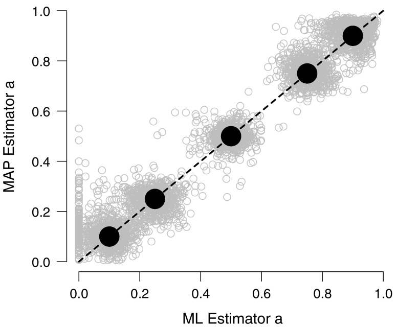
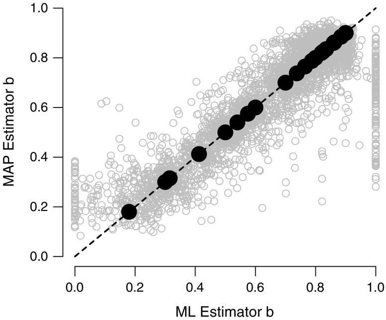
As expected, the correlations between the MAP and ML estimators are close to one for both a and b (Figs. 5 and 6). Generally, both methods seem to have similar variances. However, the ML estimator shows some problems for both a and b parameters: Some of the estimates are local optima around zero or one. The MAP estimator does not show this problem. Table 2 shows the mean error and corresponding standard deviation for both the ML and MAP estimators as a function of sample size. Overall, the MAP estimator is a reasonable choice to fit the information gain model. However, caution should be exercised, especially when estimating small values (e.g., a and b <.1). Simulations have shown that accurate estimation is difficult for small values due to a flat ridge in the likelihood space in that region.
Fig. 5.
Relation between MAP estimates and ML estimates for parameter a. The solid black circles indicate the true, data-generating values of the a parameter, whereas the open gray circles indicate the estimated values. Note that both estimators are highly correlated, but the MAP estimator is more robust
Fig. 6.
Relation between MAP estimates and ML estimates for parameter b. The solid black circles indicate the true, data-generating values of the b parameter, whereas the open gray circles indicate the estimated values. Note that both estimators are highly correlated, but the MAP estimator is more robust
Table 2.
Mean error and corresponding standard deviation of ML and MAP estimators for a and b parameters as function of sample size
| Error a | Error b | |||||||
|---|---|---|---|---|---|---|---|---|
| MAP | MLE | MAP | MLE | |||||
| n | mean | SD | mean | SD | mean | SD | mean | SD |
| 20 | 0.003 | 0.144 | –0.010 | 0.152 | –0.083 | 0.172 | –0.070 | 0.198 |
| 40 | 0.004 | 0.139 | –0.004 | 0.143 | –0.082 | 0.167 | –0.072 | 0.184 |
| 60 | 0.003 | 0.138 | –0.006 | 0.141 | –0.080 | 0.166 | –0.074 | 0.180 |
| 80 | 0.004 | 0.137 | –0.003 | 0.139 | –0.082 | 0.164 | –0.076 | 0.174 |
| 100 | 0.003 | 0.136 | –0.004 | 0.138 | –0.082 | 0.163 | –0.076 | 0.173 |
MAP shows a slightly higher bias, but a consistently smaller standard error than MLE.
Hierarchical Bayes
Contrary to the nonhierarchical models, the following code accounts for two levels in Wason task data. This is useful if Wason card selection data come from different experiments, for example.

The variable  should be a matrix of the number of trials that each card was selected, with four columns corresponding to the four cards (p, not-p, q, not-q). The rows of the matrix correspond to the experiment to which the trials belong. Variable
  is a vector of the total number of trials for each experiment. Again, ε is the error probability that the conditional rule does not hold in the dependence model.
Practical illustration
We will now illustrate the MLE and Bayesian estimation procedures using data from the meta-analysis by Oaksford and Chater (1994, their Table 2). Our Fig. 1 shows the mean selection proportion and corresponding standard deviation for each of the four cards. As discussed above, participants most frequently select the p and q cards, whereas they hardly select the logically correct not-q card. The means are based on 34 conditions from a total of 28 experiments involving the abstract Wason selection task. For each condition, the number of selected cards is available for all four cards. In total, 845 people participated. Although some conditions are part of the same experiment, only two levels of analysis will be considered here: condition and trial. We first fit the information gain with the two nonhierarchical procedures MLE and nonhierarchical Bayes, and then apply the hierarchical Bayes model. For the Bayesian models, we will calculate posterior predictives in order to assess goodness of fit.
Despite the hierarchical nature of the data, both standard MLE and nonhierarchical Bayes can only deal with one level at a time. Our goal here is to estimate the a and b in the population. Although the parameters could be estimated for each of the 34 conditions separately and then combined in a (weighted) average, here we ignore the condition level altogether, so that estimating a and b only requires the total number of trials (845) and the number of times each card is selected (p, 754; not-p, 137; q, 522; not-q, 215). The code used for this illustration is available online.
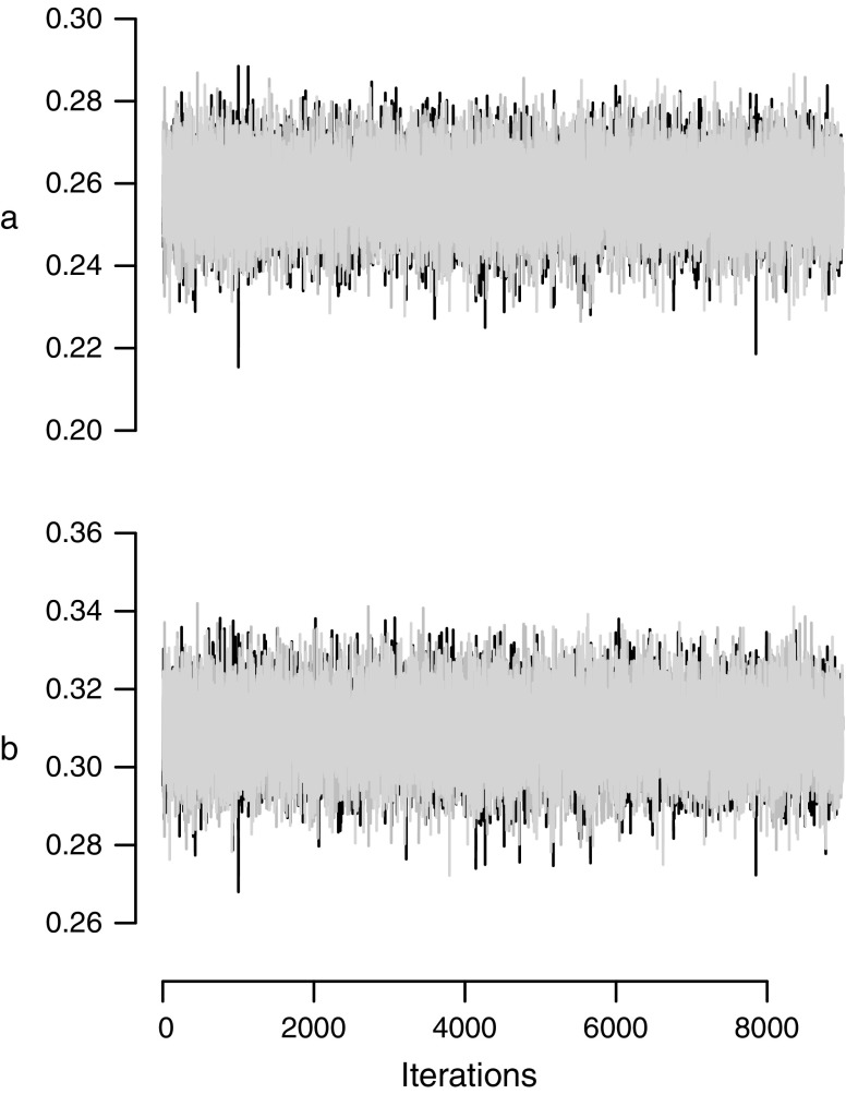
Using the MLE procedure described above on the meta-analysis data, we obtained point estimates a = .26 and b = .31. Although bootstrapping procedures exist to compute MLE confidence intervals, this would require sampling from individual trials. Next, we applied the nonhierarchical Bayesian procedure using MCMC in WinBUGS. The result of MCMC estimation is a number of chains with a series of parameter values. After an initial burn-in period, these values should converge to the posterior distribution. It is therefore important to confirm, before interpreting the MCMC results, whether the MCMC chains have converged. Although convergence cannot be proven, if chains with different starting points become indistinguishable after an initial burn-in period, this is a strong indication for convergence. This is the case in Fig. 7. All three chains are both mixed and stable. After burn-in, the different chains oscillate around the same mean with similar variances, despite differences in starting point. If different chains do not converge toward the same mean (i.e., are not mixed) or show erratic behavior (i.e., are not stable), the results should not be trusted. In that case, a longer burn-in period, more data, or adjustments to the model might be in order.
Fig. 7.
MCMC chains for the parameters from the nonhierarchical Bayesian model as applied to the data from the meta-analysis by Oaksford and Chater (1994). Note that the chains are indistinguishable, indicating convergence to the posterior distribution
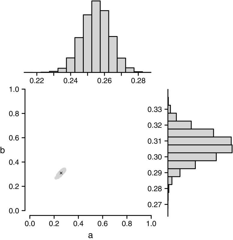
As expected, the a and b MAP estimates are very similar to the ML estimates: a = .26 and b = .31. Unlike MLE, Bayesian estimation makes it easy to compute a 95% confidence interval from the posterior parameter distributions: a ∈ [.24, .27], and b ∈ [.29, .33]. The bivariate posterior distribution (Fig. 8) shows that the a and b estimates are highly correlated (r = .87, p < .001).
Fig. 8.
Posterior distributions for the a and b parameters from the nonhierarchical Bayesian model as applied to the data from the meta-analysis by Oaksford and Chater (1994). The cross indicates the mean of the bivariate distribution
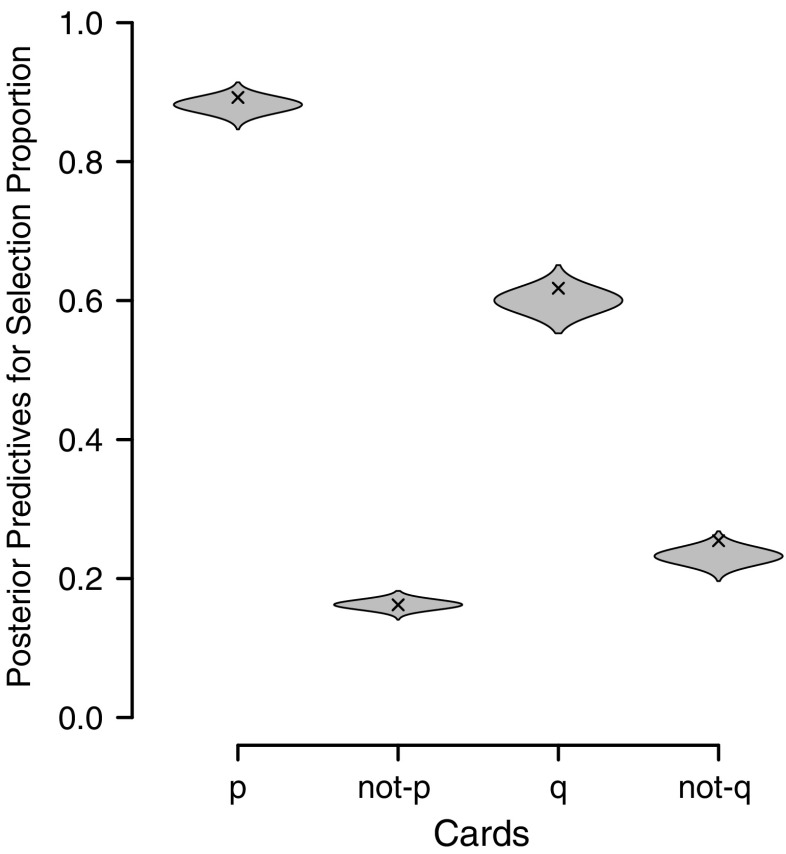
To check model fit, we consider the posterior predictives (Gelman, Carlin, Stern, & Rubin, 2004)—that is, model predictions for card selections based on samples from the joint posterior distribution. Since the joint posterior distribution represents the uncertainty in the parameter estimates, this uncertainty is reflected in the posterior predictives. If a model fits well, the empirical data are close to the posterior predictives. Figure 9 shows violin plots (Hintze & Nelson, 1998) of the posterior predictives for each card with the corresponding empirical probabilities. A violin plot is similar to a box plot, but instead of merely showing the different quartiles of a distribution, it provides a compact mirrored image of the full distribution.
Fig. 9.
Posterior predictives from the nonhierarchical Bayesian model as applied to the data from the meta-analysis by Oaksford and Chater (1994). Violin plots display the predicted selection proportions for each of the four cards. The crosses indicate the empirical values. The model predictions match the empirical data reasonably well
The violin plots in Fig. 9 indicate that the variance in the posterior distribution is relatively low. Moreover, the empirical means are contained within the posterior distributions, suggesting that the model fit is acceptable.
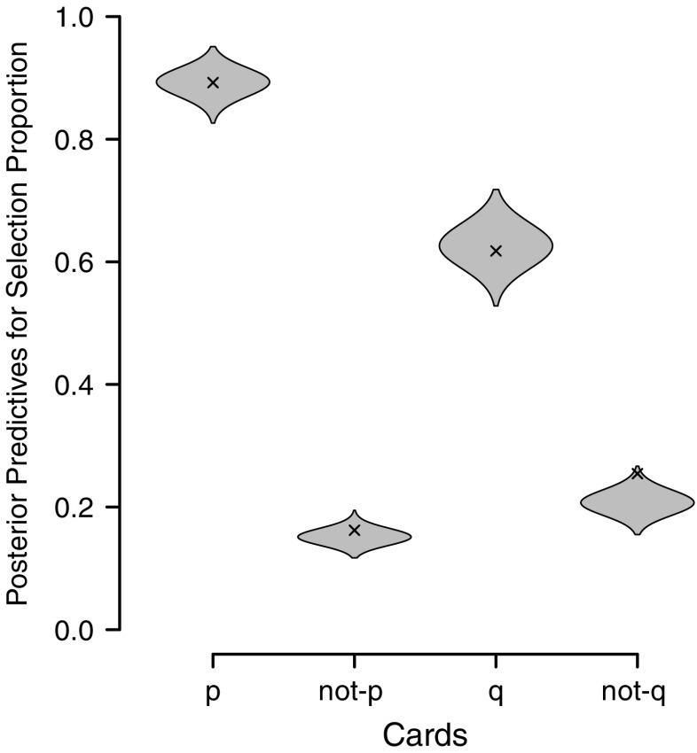
Finally we analyze the data from Oaksford and Chater (1994) using the hierarchical Bayes procedure. Now the data consist of a matrix of card selections per card and experiment, on one hand, and a vector with the number of trials in each experiment, on the other hand. Although the hierarchical procedure allows estimation of a and b for each experiment individually, we focus here on the population values a 0 and b 0 for ease of comparison with the nonhierarchical methods. Because this model takes the hierarchical structure of the data into account, the MAP estimates are somewhat different from the estimates of the two previous procedures: a 0 = .24 ∈ [.20, .27] and b 0 = .28 ∈ [.25, .32] (95% confidence intervals). The confidence intervals are larger due to the extra latent variables per experiment, which increase the uncertainty in the posterior estimates. Figure 10 shows the posterior predictives. As in Fig. 9, the empirical means are contained within the posterior distributions, and this suggests that the model fit is acceptable.
Fig. 10.
Posterior predictives from the hierarchical Bayesian model as applied to the data from the meta-analysis by Oaksford and Chater (1994). Violin plots display the predicted selection proportions for each of the four cards. The crosses indicate the empirical values. The model predictions match the empirical data reasonably well
Discussion
We have presented two Bayesian procedures to estimate the parameters of the information gain model and compared them to an ML estimation procedure. One advantage of a Bayesian estimation procedure is that it produces posterior distributions instead of point estimates. Although confidence intervals can be computed for ML estimators using bootstrapping or the Hessian, confidence intervals are automatically obtained in Bayesian estimation. Besides giving an indication of the plausible range of the estimates, the uncertainty of the parameter estimates can also be used to compute posterior predictives for particular aspects of the data. Posterior predictives provide the range of results that the model is likely to produce on the basis of the estimated parameters. The fit of a model can be assessed by comparing the posterior predictives with the observed data. Furthermore, Bayesian modeling in general, and the WinBUGS modeling language in particular, make it easy to extend models by adding a hierarchical structure. Hierarchical models account for multilevel dependencies, resulting in estimates that are more accurate than their nonhierarchical counterparts, provided that the hierarchical assumptions are valid.
In Bayesian estimation, posterior distributions always depend on the prior distributions. However, prior distributions reflect explicit assumptions, which might be implicit in other estimation paradigms. Assuming uniform priors, for example, the mode of the posterior distribution (MAP) is equivalent to the ML estimator. Consequently, if a uniform prior is deemed unreasonable, so is the ML estimator. In addition, for the information gain model, our MAP procedure is more robust with respect to local optima than our MLE procedure. A noninformative prior is not necessary, though. If knowledge from other data sets is available, an informative prior could be used to take this information into account. For larger sample sizes, the exact prior distributions are less important, since in that case they exert little influence on the analysis. Overall, the Bayesian paradigm provides a flexible, powerful, and transparent approach to parameter estimation.
In this article, we have focused exclusively on parameter estimation. However, the Bayesian framework can certainly be extended to hypothesis testing or model selection (Dennis, Lee, & Kinnell, 2008; Jeffreys, 1961; Kass & Raftery, 1995; Liang, Paulo, Molina, Clyde, & Berger, 2008; Wagenmakers, Lodewyckx, Kuriyal, & Grasman, 2010). For instance, one might want to examine whether subgroups of participants (e.g., children with ADHD, children with autism, and typically developing children) perform the same on the Wason card selection task, in the sense that these different subgroups have identical parameter values. This question can be formalized by contrasting two models, a null model H 0 in which the parameters are identical across subgroups and an alternative model H 1 in which the parameters are allowed to vary. A precise quantification of the evidence that the data provide for H 0 versus H 1 involves the computation of a weighted average likelihood, a discussion of which can be found elsewhere (see, e.g., Kass & Raftery, 1995; Wagenmakers et al., 2010).
A disadvantage of Bayesian modeling is that it is relatively computer intensive. The extra information obtained from the posterior distribution, as compared to a point estimate, comes at a computational price, since many iterations are required to ensure convergence of the MCMC chains and to obtain a histogram of values that accurately reflects the posterior distribution. However, with current computer power, these limitations have become less problematic.5
We illustrated our Bayesian estimation procedure by estimating the parameters of the information gain model using data from a meta-analysis of the Wason task (Oaksford & Chater, 1994). As expected, the MAP estimates were similar to the ML estimates. Furthermore, the posterior predictives matched the observed data reasonably well. The estimation procedure is simple, and our code offers the first publicly accessible implementations of the information gain model. Researchers can now easily estimate parameters of the information gain model for their own data, using either hierarchical or nonhierarchical specifications. We hope that the availability of easy-to-use Bayesian estimation routines will facilitate the application of formal models to data from human reasoning research.
Electronic supplementary material
Below is the link to the electronic supplementary material.
(ZIP 10.7 kb)
Author Note
This research was supported by a grant from the Dutch Ministry of Education, Culture, and Science and by a Vidi grant from the Dutch Organization for Scientific Research (NWO).
Supplemental materials
The data from Oaksford and Chater (1994), as well as the R and WinBUGS code and example MCMC chains referred to in this article, may be downloaded along with this article.
Open Access
This article is distributed under the terms of the Creative Commons Attribution Noncommercial License which permits any noncommercial use, distribution, and reproduction in any medium, provided the original author(s) and source are credited.
Appendix A Mathematics of the information gain model
Here we present the mathematical details of the information gain model as discussed in Oaksford and Chater (2003). The probability of selecting card  is
is
 |
1 |
The numbers 2.37 and 9.06 were determined from empirical data (Hattori, 1999, as cited in Oaksford & Chater, 2003). SEIG (x i) is the scaled expected information gain of card x i:
 |
2 |
where EIG, the expected information gain of turning a card, depends on the card. Here we show how to compute the expected information of the p card. The expected information of the other cards is computed similarly.
For the p card,
 |
3 |
where Pr(q | p) is the probability of q on one side given p on the other side. IG(p q) is the information gained by turning a p card and finding a q card on the other side. Computation of IG(p q) will be discussed later. First we show how to compute the conditionals.
Conditionals such as Pr(q | p) can be computed by marginalizing over both models:
 |
4 |
where M D is the dependence model and M I the independence model. The prior probabilities of the models are assumed to be equal. So
 |
5 |
The information gain of seeing q after turning a p card is the difference between the uncertainty before and after turning the p card:
 |
6 |
where I(M) is the a priori uncertainty about the model (dependence model M D or independence model M I) as measured by the Shannon–Wiener information index. I(M | p q) is the uncertainty concerning the true model after turning the p card and finding q on the other side. The two information values are calculated below.
 |
7 |
where i indexes over the dependence and independence models. Since, a priori, both models are equally probable (e.g.,  ), we obtain the maximum uncertainty of 1.
The conditional information is computed similarly.
 |
8 |
where the probability of model i given card p q [i.e., Pr(M i | p q)] can be obtained with the help of Bayes’s theorem:
 |
9 |
where the prior probability of each model is assumed to be .5. The probability of seeing a q after turning a p card given model i [i.e., Pr(q | p, M i)] can be computed by marginalizing the joint conditional probabilities:
 |
10 |
where the joint conditional probabilities are depicted in Table 3. The marginal probabilities Pr(x | M i) are assumed to be independent of the model and can therefore be easily derived from parameters a and b, which are the prior probabilities of p and q:
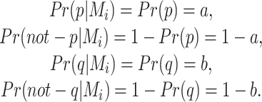 |
11 |
Table 3.
Contingency table of joint probabilities of card combinations under the dependence and independence models
| q | not-q | |
|---|---|---|
| Dependence model | ||
| p | a(1 − ε) | aε |
| not-p | b − a(1 − ε) | 1 − b(a − ε) |
| Independence model | ||
| p | ab | a(1 – b) |
| not-p | b(1 – a) | (1 – b)(1 – a) |
a = Pr(p), b = Pr(q), ε = Pr(not − q | p)
Appendix B Uniform priors on (a, b)
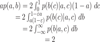
Since a and b are the parameters of interest in the information gain model, we have used an uninformative prior for the joint distribution of (a, b). In this section, we show that if u and c are both independent and uniformly distributed and  , then p(a, b) = 2 and thus is uniformly distributed.
The definition of a is an example of inverse transform sampling:  . The cumulative distribution function for a is therefore
  . Differentiation results in the probability density function p(a) = 2(1 – a).
Let p(a) = 2(1 – a) and p(c) = 1. Furthermore, a and c are assumed to be independent. Therefore,  . Under these assumptions, the prior of p(a, b) = 2, and is therefore uniform:
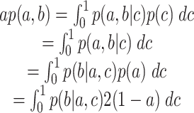 |
12 |
Although p(b | a, c) is a deterministic and therefore discrete function, we can define it as a continuous delta Dirac function around point  . In other words, if
  , then
  ; otherwise,
  . Furthermore,
  . Substituting
  , we obtain:
 |
13 |
This proves that p(a, b) is indeed uniformly distributed.
Footnotes
Klauer et al. (2007) combined inferential processes and independent processes in a single, comprehensive quantitative model.
WinBUGS can be obtained from www.mrc-bsu.cam.ac.uk/bugs.
R is a free software environment for statistical computing that can be obtained from www.r-project.org.
www.springerlink.com and www.svenstringer.com, respectively.
For example, on a 64-bit Windows computer with an Intel Duo Core processor at 2.2 GHz with 4 GB RAM, it takes 126 s to estimate the nonhierarchical information gain model with three chains of 10,000 iterations each.
References
- Cavagnaro DR, Myung JI, Pitt MA, Kujala J. Adaptive design optimization: A mutual information-based approach to model discrimination in cognitive science. Neural Computation. 2010;22:887–905. doi: 10.1162/neco.2009.02-09-959. [DOI] [PubMed] [Google Scholar]
- Cavagnaro, D. R., Pitt, M. A., & Myung, J. I. (in press). Model discrimination through adaptive experimentation. Psychonomic Bulletin & Review. [DOI] [PMC free article] [PubMed]
- Chater N, Oaksford M. Information gain and decision-theoretic approaches to data selection: Response to Klauer. Psychological Review. 1999;106:223–227. doi: 10.1037/0033-295X.106.1.223. [DOI] [Google Scholar]
- Dennis SJ, Lee MD, Kinnell A. Bayesian analysis of recognition memory: The case of the list-length effect. Journal of Memory and Language. 2008;59:361–376. doi: 10.1016/j.jml.2008.06.007. [DOI] [Google Scholar]
- Efron B, Tibshirani RJ. An introduction to the bootstrap. New York: Chapman & Hall; 1993. [Google Scholar]
- Evans, J. St. B.T., & Over, D. E. (2004). If: Supposition, pragmatics, and dual processes. Oxford: Oxford University Press.
- Gamerman D, Lopes HF. Markov chain Monte Carlo: Stochastic simulation for Bayesian inference. Boca Raton: Chapman & Hall/CRC; 2006. [Google Scholar]
- Gelman A, Carlin JB, Stern HS, Rubin DB. Bayesian data analysis. 2. Boca Raton: Chapman & Hall/CRC; 2004. [Google Scholar]
- Gelman A, Rubin DB. Inference from iterative simulation using multiple sequences (with discussion) Statistical Science. 1992;7:457–472. doi: 10.1214/ss/1177011136. [DOI] [Google Scholar]
- Gilks WR, Richardson S, Spiegelhalter DJ, editors. Markov chain Monte Carlo in practice. Boca Raton: Chapman & Hall/CRC; 1996. [Google Scholar]
- Gilks WR, Thomas A, Spiegelhalter DJ. A language and program for complex Bayesian modelling. The Statistician. 1994;43:169–177. doi: 10.2307/2348941. [DOI] [Google Scholar]
- Hattori M. The effects of probabilistic information in Wason’s selection task: An analysis of strategy based on the ODS model. Proceedings of the Second International Conference on Cognitive Science. 1999;16:623–626. [Google Scholar]
- Hattori M. A quantitative model of optimal data selection in Wason’s selection task. The Quarterly Journal of Experimental Psychology. 2002;55A:1241–1272. doi: 10.1080/02724980244000053. [DOI] [PubMed] [Google Scholar]
- Hintze JL, Nelson RD. Violin plots: A box plot-density trace synergism. American Statistician. 1998;52:181–184. doi: 10.2307/2685478. [DOI] [Google Scholar]
- Jeffreys H. Theory of probability. Oxford: Oxford University Press; 1961. [Google Scholar]
- Kass RE, Raftery AE. Bayes factors. Journal of the American Statistical Association. 1995;90:773–795. doi: 10.2307/2291091. [DOI] [Google Scholar]
- Klauer KC. On the normative justification for information gain in Wason’s selection task. Psychological Review. 1999;106:215–222. doi: 10.1037/0033-295X.106.1.215. [DOI] [Google Scholar]
- Klauer KC, Stahl C, Erdfelder E. The abstract selection task: New data and an almost comprehensive model. Journal of Experimental Psychology. Learning, Memory, and Cognition. 2007;33:680–703. doi: 10.1037/0278-7393.33.4.680. [DOI] [PubMed] [Google Scholar]
- Kruschke JK. What to believe: Bayesian methods for data analysis. Trends in Cognitive Sciences. 2010;14:293–300. doi: 10.1016/j.tics.2010.05.001. [DOI] [PubMed] [Google Scholar]
- Lee, M. (in press). How cognitive modeling can benefit from hierarchical Bayesian models. Journal of Mathematical Psychology.
- Lee, M., & Wagenmakers, E.-J. (2010). A course in Bayesian graphical modeling for cognitive science. Freely available at the authors’ websites.
- Liang F, Paulo R, Molina G, Clyde MA, Berger JO. Mixtures of g priors for Bayesian variable selection. Journal of the American Statistical Association. 2008;103:410–423. doi: 10.1198/016214507000001337. [DOI] [Google Scholar]
- Lindley DV. Bayesian statistics, a review. Philadelphia: SIAM; 1972. [Google Scholar]
- Lunn D, Spiegelhalter D, Thomas A, Best N. The BUGS project: Evolution, critique and future directions. Statistics in Medicine. 2009;28:3049–3067. doi: 10.1002/sim.3680. [DOI] [PubMed] [Google Scholar]
- Lunn DJ, Thomas A, Best N, Spiegelhalter D. WinBUGS—A Bayesian modelling framework: Concepts, structure, and extensibility. Statistics and Computing. 2000;10:325–337. doi: 10.1023/A:1008929526011. [DOI] [Google Scholar]
- Myung IJ. Tutorial on maximum likelihood estimation. Journal of Mathematical Psychology. 2003;47:90–100. doi: 10.1016/S0022-2496(02)00028-7. [DOI] [Google Scholar]
- Nelson JD. Finding useful questions: On Bayesian diagnosticy, probability, impact, and information gain. Psychological Review. 2005;112:979–999. doi: 10.1037/0033-295X.112.4.979. [DOI] [PubMed] [Google Scholar]
- Oaksford M, Chater N. A rational analysis of the selection task as optimal data selection. Psychological Review. 1994;101:608–631. doi: 10.1037/0033-295X.101.4.608. [DOI] [Google Scholar]
- Oaksford M, Chater N. The probabilistic approach to human reasoning. Trends in Cognitive Sciences. 2001;5:349–357. doi: 10.1016/S1364-6613(00)01699-5. [DOI] [PubMed] [Google Scholar]
- Oaksford M, Chater N. Optimal data selection: Revision, review, and reevaluation. Psychonomic Bulletin & Review. 2003;10:289–318. doi: 10.3758/BF03196492. [DOI] [PubMed] [Google Scholar]
- Oaksford M, Chater N. Bayesian rationality: The probabilistic approach to human reasoning. Oxford: Oxford University Press; 2007. [DOI] [PubMed] [Google Scholar]
- Oberauer K, Wilhelm O, Diaz RR. Bayesian rationality for the Wason selection task? A test of optimal data selection theory. Thinking and Reasoning. 1999;5:115–144. doi: 10.1080/135467899394020. [DOI] [Google Scholar]
- Sheu C-F, O’Curry SL. Simulation-based Bayesian inference using BUGS. Behavior Research Methods, Instruments, & Computers. 1998;30:232–237. doi: 10.3758/BF03200649. [DOI] [Google Scholar]
- Stenning K, van Lambalgen M. Human reasoning and cognitive science. Cambridge: MIT Press; 2008. [Google Scholar]
- van der Vaart AW. Asymptotic statistics. Cambridge: Cambridge University Press; 1998. [Google Scholar]
- Wagenmakers E-J, Lodewyckx T, Kuriyal H, Grasman R. Bayesian hypothesis testing for psychologists: A tutorial on the Savage–Dickey method. Cognitive Psychology. 2010;60:158–189. doi: 10.1016/j.cogpsych.2009.12.001. [DOI] [PubMed] [Google Scholar]
- Wason PC. Reasoning. In: Foss BM, editor. New horizons in psychology. Harmondsworth: Penguin; 1966. [Google Scholar]
- Wetzels R, Lee MD, Wagenmakers E-J. Bayesian inference using WBDev: A tutorial for social scientists. Behavior Research Methods. 2010;42:884–897. doi: 10.3758/BRM.42.3.884. [DOI] [PubMed] [Google Scholar]
Associated Data
This section collects any data citations, data availability statements, or supplementary materials included in this article.
Supplementary Materials
(ZIP 10.7 kb)


