Abstract
Background
Discovery of biomarkers that are correlated with therapy response and thus with survival is an important goal of medical research on severe diseases, e.g. cancer. Frequently, microarray studies are performed to identify genes of which the expression levels in pretherapeutic tissue samples are correlated to survival times of patients. Typically, such a study can take several years until the full planned sample size is available.
Therefore, interim analyses are desirable, offering the possibility of stopping the study earlier, or of performing additional laboratory experiments to validate the role of the detected genes. While many methods correcting the multiple testing bias introduced by interim analyses have been proposed for studies of one single feature, there are still open questions about interim analyses of multiple features, particularly of high-dimensional microarray data, where the number of features clearly exceeds the number of samples. Therefore, we examine false discovery rates and power rates in microarray experiments performed during interim analyses of survival studies. In addition, the early stopping based on interim results of such studies is evaluated. As stop criterion we employ the achieved average power rate, i.e. the proportion of detected true positives, for which a new estimator is derived and compared to existing estimators.
Results
In a simulation study, pre-specified levels of the false discovery rate are maintained in each interim analysis, where reduced levels as used in classical group sequential designs of one single feature are not necessary. Average power rates increase with each interim analysis, and many studies can be stopped prior to their planned end when a certain pre-specified power rate is achieved. The new estimator for the power rate slightly deviates from the true power rate but is comparable to other estimators.
Conclusions
Interim analyses of microarray experiments can provide evidence for early stopping of long-term survival studies. The developed simulation framework, which we also offer as a new R package 'SurvGenesInterim' available at http://survgenesinter.R-Forge.R-Project.org, can be used for sample size planning of the evaluated study design.
Background
A frequent objective of cancer related studies is to detect genes or biomarkers that can predict the outcome of therapy. The hardest criterion of success for therapies is the survival of patients. To identify predictive genes, the expression levels in samples of tumor or normal tissue are measured by DNA microarrays before the therapy is applied. Then, expression levels are compared to survival data of the patients. Usually, tissue samples are only available at distinguished points in time and it can take several years until the full planned sample size is available and follow-up is complete. In such long-lasting studies it would be beneficial to obtain interim results already before their planned end. An early detection of survival related genes within an interim analysis would for example allow their further laboratory validation before the end of the study. In addition, if an interim analysis provides evidence for the early stopping of the study it would save time and costs and would spare further patients to be involved or allow better treatment. Classically, interim analyses are performed in studies of group sequential designs. In such designs, interim analyses are performed when a certain fraction of the full planned sample size N has been reached, for example when 1/3 · N and 2/3 · N samples are available. There are numerous articles that deal with group sequential designs in the case of one single feature, e.g. [1,2]. As the repeated testing of the same hypothesis by interim analyses is one form of multiple testing and thus inflates the overall type I error [3], both articles propose reduced significance levels to solve this problem. DNA microarray data, however, comprise expression levels for thousands of genes, meaning that there are more features than available samples. For this case of high-dimensional data there have been very few approaches published to date. Marot and Mayer [4], for example, propose a method for combining p-values from several independent microarray analyses and show that the overall false discovery rate is not inflated when testing repeatedly a large number of hypothesis. A similar result was obtained by Posch et al. [5]. We make use of these results and apply them for studies in which survival data is correlated with gene expression data in interim analyses. In order to detect the survival related genes, we use gene-wise Cox-regression analyses [6].
An important issue in interim analyses of multiple features is the choice of a stopping criterion. In the case of testing one single feature, the study is simply stopped when a significant result is observed. Similarly, Victor and Hommel [7] use gene-wise stopping rules in the case of high-dimensional microarray data. Marot and Mayer [4] and Posch et al. [5] propose to stop the study when a certain proportion of true positive genes has been detected. We pick up the latter idea and derive an estimator for the proportion of true positive findings This new estimator is compared to a variant based on [8] and to an estimator proposed in [4].
The article is structured as follows. The study design, the detection of survival-related genes, the problem of performing interim analyses in the case of multiple hypothesis testing, and the stop criterion are detailed in the Methods section. Subsequently, a simulation study evaluates the behavior of the false discovery rate and of the estimator for the proportion of true positive detections. The simulation study covers several settings of survival-focused microarray experiments with interim analyses. After presenting the results from these simulations, we apply our methods to gene expression data from a breast cancer study van de Vijver et al. [9]. Parameters from this breast cancer study are used one more simulation presented subsequently. Finally, a discussion on the results follows, and further ideas are given.
Methods
This section starts with an illustration of the particular study design we are considering in this article. As survival is a special focus of this work, we detail afterwards the methods for the detection of survival-related genes. Next, an overview of common methods for multiple hypothesis testing and their application in group sequential interim analyses is given. In this context, we also describe rules for the early stopping of such studies.
First, let us introduce the basic notation. Let N be the total number of subjects that would be involved if the study was not stopped after any interim analysis. For each of the relating tissue samples the expression levels of d genes are measured by means of DNA microarrays. We denote the complete (d × N) data matrix with all genes and all samples by X. As typical for microarray data, each row represents one gene and each column represents one sample. Thus, xij denotes the expression level of gene i in the tissue sample of subject j (i = 1, ..., d; j = 1, ..., N). An overview of all notations is given in Table 6.
Table 6.
Mathematical Notation
| 1. Patient Data | |
| N | samples |

|
anticipated length of the recruitment part of the study |
| a = (a1, ..., aN) | arrival times |
| where ai ~ U(0, l1), i = 1, ..., N | |
| l1 = max(a) | length of the recruitment part |
| l2 | length of the follow-up part |
| L = l1 + l2 | study length |
| M1 | number of analyses within l1 |
| M2 | number of analyses within l2 |
| M = M1 + M2 | number of analyses |
| t = (t1, ..., tN) | analysis times |
| λ | mean survival time |
| s = (s1, ..., sN) | survival times |
| where si ~ Exp(λ), i = 1, ..., N | |

|
censor variable |
where 
|
|
| 2. Gene Expression Data | |
| d | genes |
| d0 | genes not associated with survival |
| d1 | genes associated with survival |
| R | number of positive test decisions |
| FN | false negative test decisions |
| TN | true negative test decisions |
| FP | false positive test decisions |
| TP | true positive test decisions |
| τ | fraction of differentially expressed genes |

|
gene expression data |
| ϑ | tuning parameter within the estimation of the proportion of true null hypotheses |
| αBH | the level for the type I error that is adjusted according to the BH- procedure |
Study Design
Assume, the whole study is not stopped after any interim analysis. Then, the N patients will have individual arrival times a = (a1, ..., aN )', e.g. months after the begin of the study. We denote the arrival time of the last patient to enter the study by l1 = max(a). Thus, the first part of the study, during which patients are recruited, will take place in the time frame [0, l1].
Let us consider a second study episode which serves as a follow-up time of length l2, where no new patients enter the study but the patients survival data is still observed and up-dated. Thus, the length of the full study without any early stopping would be L = l1 + l2, and the time frame of the second study part would be [l1, L]. The study design is visualized in Figure 1.
Figure 1.
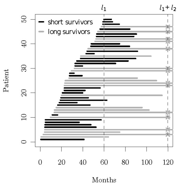
Study Design. The arrival time of each patient is marked by the left end of each horizontal bar and his death by the right end. The dashed lines represent the end of the recruitment part of the study and the end of the follow-up part, respectively. Patients marked with an 'x' have censored survival times at the final analysis.
Assume further, that M1 interim analyses are planned to take place during the first study part. An interim analysis is always performed when (1/M1) · N new samples are available. This makes sure, that the sample size in each analysis is equal. In addition, M2 interim analyses are planned for the second study part, where an interim analysis is always performed when a time proportion of (1/M2) · l2 of the planned follow-up time has passed. Thus, we chose to perform analyses at equally spaced time-steps during this second part of the study. We denote the times at which interim analyses are performed by tm (m = 1, ..., M, where M = M1 + M2).
Detecting Survival-related Genes
Disease specific survival is the hardest control for measuring the success of cancer therapies. Therefore, we modelled the survival information in dependence on the gene expression data using Cox proportional hazard regression as was proposed for example by Simon et al. [10]. Survival information consists for each patient j of a pair (sj, zj), where sj is the observed survival time of the patient, and zj ∈ {0, 1} specifies whether the patient has already died or not at the time the analysis takes place. According to the Cox-regression model, the survival information is modelled in terms of the hazard function at time t in dependence on gene i by
| (1) |
where h0 is an unspecified function of t, called the baseline hazard. The hazard function h(t) can be interpreted as the patients risk of dying in a short time frame, [t, t + ε), assuming the patient has survived thus far [11]. More precisely, the hazard function is defined as
| (2) |
where t* is the patients observed survival time [12]. The influence of gene i on survival can be determined by testing the hypothesis H0i: βi = 0 in the related Cox model. The d resulting p-values from the gene-wise survival analyses can than be adjusted for multiple testing as described below.
In general, other models than the Cox model can be considered to detect survival-related genes. Park et al. [13] for example propose to use partial least squares regression to account for the presence of covariates.
Interim Analyses of Multiple Endpoints
In each interim analysis one statistical test is performed per gene in order to detect those genes which correspond to the studied response variable (e.g. overall survival).
If the d hypotheses were all true and independent, testing each of them at the same level α, the expected number of false positive detections would be given by α · d. In whole genome microarray experiments, where d is typically about 40.000, the expected number of false positive detections would be too large to be tolerable. In multiple testing situations, it is therefore common to reduce the number of false positive decisions by controlling a pre-specified type I error rate. Note that the notion of type I error rate is not used consistently in the literature. Following Dudoit et al. [14] we will use the term type I error rate to name the superordinate concept of different types of such error rates, among which there are the family-wise error rate (FWER) and the false discovery rate (FDR).
In microarray experiments the FDR, introduced by Benjamini and Hochberg [15], is the most commonly considered type I error rate. The FDR is defined as the expected proportion of false positives among all positive test decisions, i.e. FDR = E(FP/R), where R > 0 denotes the total number of rejected null-hypotheses. The proportion of false positives (FP) among all positives itself is also known as false discovery proportion (FDP = FP/R). In the special case that R = 0, i.e. no positive test decisions were found, the FDP as well as the FDR are defined to be zero.
The FDR can be controlled by adjusting the raw p-values resulting from the gene-wise tests. The adjusted p-values are then compared with a pre-specified level α of the FDR that is desired to be controlled. We denote the unadjusted p-value for gene i by pi and the respective adjusted p-value by  . In our simulation study, we consider the adjusting procedure proposed by Benjamini and Hochberg [15]. Other adjusting procedures are detailed in [14].
Alternatively to comparing the adjusted p-values with the pre-specified FDR-level α, genes can be selected by comparing the raw p-values with adjusted α-levels. According to the procedure in [15], the raw p-values are ordered by increasing size, i.e. p(1) ≤ p(2) ≤ ... ≤ p(d), and the largest k (k = 1, ..., d) for which p(k) ≤ (k/d) α has to be determined. All hypothesis associated with p(1) to p(k) are then rejected. We denote the adjusted α-level that corresponds to this largest value of k by αBH.
Similar as in multiple hypothesis testing, the control of type I error rates is an important issue in group sequential interim analyses. In clinical trials on one single feature (for example when only one gene would be tested), interim analyses have been studied in-depth. As was shown by Armitage et al. [3], performing interim analyses increases the probability for making a type I error. In order to avoid such an increase and to maintain a pre-specified type I error, the tests at each interim analysis are performed at lower nominal levels  (m = 1, ..., M). The first authors who proposed α-level adjustments for group sequential interim analyses were Pocock [1] and O'Brien and Fleming [2].
At first glance, performing interim analyses in microarray experiments seems to require two adjustments. One to account for the interim analyses and one to account for multiple testing. However, the two recently published articles by Posch et al. [5] and by Marot and Mayer [4], show that the adjustment for interim analyses can be omitted, when d is large, while the FDR remains controlled. The result in [4] is based on the observation that the correlation between a single p-value and the empirical distribution of all p-values approaches zero when d gets large. The results in [5] are based on the findings of Storey et al. [16] who proved that, under certain assumptions,
| (3) |
This holds for each interim analysis independently. Let  denote the random interim analysis where the study is stopped. Posch et al. [5] proved that equation (3) holds also at this interim analysis
  , since
| (4) |
With equations (3) and (4) and the Lemma of Fatou it follows that the FDR is controlled asymptotically when d gets large.
This argumentation is not valid under the global null hypothesis (no gene significant), but it is also possible to extend the argumentation to the case of the global null hypothesis [5].
When performing interim analyses in experiments with multiple endpoints, one has to decide which data to base the interim analysis on. We decided to use all available accumulated data in each interim analysis.
This approach makes sure, that every analysis uses the maximal available data. However, one has to be aware of its drawback: it requires renormalization of the data in each analysis which leads to inconsistencies across the interim analyses.
Stopping Rules
One important point in studies with planned interim analyses is the stop criterion. Each interim analysis provides the possibility to stop the study prior to its planned end, entailing the mentioned ethical and financial benefits. In studies on one single feature the study is usually stopped if that feature is found to be significant. In studies on a large number of features one could stop the study as soon as a pre-specified fixed number of features has been found to be significant. In the case of microarray analyses, this criterion might be useful when the number of genes that can be further validated by laboratory experiments is limited by costs or time.
Here, we follow the approach of Marot and Mayer [4] who consider as stop criterion the achieved proportion of detected true positives, the so called average power rate (APR)
| (5) |
where d1 is the number of non-true null hypothesis. At each interim analysis the achieved APR is estimated and the study is stopped if this estimate exceeds a predefined level, e.g. 80%. In the case of d1 = 0 the APR is defined to be zero.
We employ a new estimator of the APR, similar to the FDR-estimator of Storey and Tibshirani [8] which is based on the following relations:
 |
(6) |
The three components E[R], E[FP] and E[d1] can be estimated as in [8] which is shown in the following. The expectation of R can simply be estimated by the observed number of rejected hypothesis, i.e.
| (7) |
The estimation of E[FP] is based on the fact, that p-values belonging to true null-hypotheses are uniformly distributed within [0,1]. Thus, the probability that a p-value which belongs to a true null-hypothesis is smaller than a threshold t (t ∈ [0,1]) is exactly t. Therefore, if the significance level is chosen to be α' = t and d0 null hypotheses are true, E[FP] can be estimated by
| (8) |
where π0 is the fraction of true null hypothesis. For α' one can for example choose αBH as defined in the previous subsection. The unknown fraction π0 of true null hypotheses can be estimated by
| (9) |
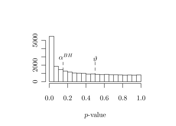
Here, ϑ serves as a tuning parameter that balances bias versus variance. For a well chosen ϑ, the p-values in [ϑ, 1] will belong 'mostly' to true null-hypotheses, and therefore equation (9) estimates the fraction of true null-hypotheses. Again, the argument is the uniform distribution of p-values belonging to true null-hypotheses. See Figure 2 for graphical illustration.
Figure 2.
Empirical p-Value Distribution from the Breast Cancer Data. The tuning parameter ϑ is used within the estimation of the fraction π0 of true null hypothesis. The multiple testing adjusted α-level is marked with αBH.
According to our simulations (see below) setting ϑ = 0.5 results in a good estimate  . Other automated ways to choose ϑ have been proposed in [17] and [8]. In both cases the estimate of π0 is used to estimate not the APR but the FDR. Storey [17] calculates the mean squared error of the FDR estimator for a range of values of ϑ and takes the one minimizing this MSE. The calculation of this MSE thereby is in turn based on a plug-in estimate of the FDR. The method presented in [8] does not need the FDR but is based on
  only. The underlying observation is, that the bias in the estimator of π0 vanishes in the extreme choice ϑ = 1. Thus, the approach there is, to set
  .
.
A non-parametric estimator of π0 is given by Langaas et al. [18]. Based on this estimator and on the empirical distribution of the p-values Marot and Mayer [4] construct an APR estimator analog to the beta uniform model presented by [19].
In any case, the expectation of d1 can be estimated by
| (10) |
such that the final estimator for the APR is given by
| (11) |
We will use  to denote the estimator that results from setting ϑ = 0.5 and
  (S) to denote the estimator which is based on the procedure for estimating π0 presented in [8]. The estimator by Marot and Mayer [4] will be denoted by
  (L).
(L).
Results
Simulation Study
Data Generation and Settings
In order to simulate a study of the design proposed in subsection 'Study Design' we set the following parameters. At first, we chose the total number of samples to be N = 50. Furthermore, we set the intended length of the recruitment part of the study  and the length of the follow-up part to be 60 months, each, i.e.
  . We assume that the arrival times a are distributed uniformly during this first part. Thus, they were drawn from
  . The patients' survival times were assumed to follow an exponential distribution Exp(1/λ), where λ is the mean survival time. Here, we set λ = 60 months.
As we wanted to generate a set of genes which correspond to the simulated survival times, we split the individuals into two groups. The one group comprises the subjects with survival smaller than the specified λ the other group the subjects with equal or longer survival times than λ. The gene expression data for the two groups were then drawn from multivariate normal distributions Nd(μk, Σ), k = 1, 2. Expression levels were simulated for d = 10000 genes. The different mean vectors of the two groups represent the differentially expressed genes between subjects with short or long survival. For both groups, the same covariance matrix Σ with an autoregressive structure was generated. This structure images the fact that some genes are highly correlated among each other while others behave rather independent. In detail, we set
 |
(12) |
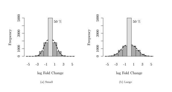
The expectation vector μ1 of the one group was set to be the null-vector, while a fraction of τ = 50% randomly chosen genes was altered in the other group. The alterations in μ2 were drawn from 'discretized' normal distributions. Larger fold changes were simulated via a higher standard deviation of this normal distribution. The structure of μ2 is illustrated in Figure 3.
Figure 3.
Simulated Log Fold Changes. Both plots display a distribution of log fold changes of the genes between short and long time survivors in the setting where 50% of all genes were not altered between both groups. Fold changes were drawn from a 'discretized' normal distribution (dashed line). (a) small fold changes, (b) large fold changes.
This way we simulate an effect of a fixed size in the gene expression depending on whether the patient belongs to the group of long-term survivors or not. Of course in biology the inverse direction is true, i.e. survival is regulated by gene expression. However, we think that for our purpose it does not matter in which order the survival and expression data are generated. In addition, it is typical in biology that a gene is either up- or down-regulated. Hence, only the direction of regulation but not the strength of regulation influences the outcome. Therefore we chose to model the relationship between single genes and survival by a discrete function and not by some continuous one.
At each interim analysis, a gene-wise Cox regression was performed to detect the survival correlated genes, and resulting p-values were adjusted to control the FDR at a level of 5%. Following the results of Marot and Mayer [4] and of Posch et al. [5], no additional adjustment for interim analyses was performed. The number of simulation runs was set to 1000 for each setting. All simulations were performed with the free software R in version 2.10 [20].
We simulated two different setups. One, where 2 interim analyses are scheduled for both study parts, i.e. M1 = M2 = 2, and one where 5 analyses are planned to take place per part, i.e. M1 = M2 = 5. In each simulation run, our power estimator described in Section 'Stopping Rules' was applied and the study was stopped when an estimated APR of 80% was achieved.
As a more extreme setting we additionally simulated in the second setup (M1 = M2 = 5) the situation of a smaller fraction τ = 5% of altered genes.
Adherence to False Discovery Rate
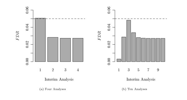
As no interim-specific adjustments were applied, the question arises, whether the pre-specified FDR-level of 5% was maintained at each analysis. Figure 4 displays the mean simulated FDR at each interim analysis in two different settings. Figure 4(a) represents the case of M = 4 analyses (i.e., 3 interim and one final), while Figure 4(b) represents the case of M = 10 analyses. Table 1 and Table 2 contain the mean and standard deviation of the FDR for these cases. Both results were obtained with the fold changes for the genes between long and short time survivors being generated as shown in Figure 3(b). The pre-specified FDR-level of 5%, indicated by the dashed line, is maintained at nearly each analysis.
Figure 4.
Simulated FDR (τ = 50%). The simulated FDR is plotted at each interim analysis in the setting where 50% of all genes were altered between both groups. (a) M = 4 analyses (3 interim and 1 final), (b) M = 10 analyses. The dashed line marks the pre-specified FDR-level of 5%.
Table 1.
Simulated FDR and Power Rate (4 Analyses)
| Analysis | ||||||||
| 1 | 2 | 3 | 4 | |||||
| mean | sd | mean | sd | mean | sd | mean | sd | |
| #found genes | 38 | 180 | 2422 | 896 | 4079 | 379 | 4232 | 290 |
| FDR | 0.051 | 0.158 | 0.028 | 0.006 | 0.027 | 0.003 | 0.027 | 0.003 |
| APR | 0.007 | 0.035 | 0.471 | 0.174 | 0.793 | 0.074 | 0.823 | 0.056 |
 |
0.017 | 0.071 | 0.515 | 0.170 | 0.803 | 0.054 | 0.829 | 0.033 |
 (S) (S) |
0.014 | 0.053 | 0.491 | 0.168 | 0.788 | 0.073 | 0.816 | 0.057 |
 (L) (L) |
0.351 | 0.133 | 0.707 | 0.077 | 0.865 | 0.038 | 0.882 | 0.025 |
The descriptive values for each interim analysis including the number detected genes, the simulated FDR, the real APR, and the APR estimates, all in the setting of τ = 50% altered genes and four interim analyses. These values correspond to Figure 4 (a) and Figure 5 (a).
Table 2.
Simulated FDR and Power Rate (10 Analyses)
| Analysis | ||||||||||
|---|---|---|---|---|---|---|---|---|---|---|
| 1 | 2 | 3 | 4 | 5 | ||||||
| mean | sd | mean | sd | mean | sd | mean | sd | mean | sd | |
| #found genes | 0 | 0 | 10 | 85 | 164 | 437 | 1033 | 928 | 2404 | 915 |
| FDR | 0.003 | 0.055 | 0.029 | 0.119 | 0.048 | 0.145 | 0.034 | 0.061 | 0.028 | 0.006 |
| APR | 0.000 | 0.000 | 0.002 | 0.016 | 0.032 | 0.085 | 0.200 | 0.180 | 0.467 | 0.178 |
 |
0.043 | 0.060 | 0.038 | 0.120 | 0.049 | 0.134 | 0.241 | 0.208 | 0.518 | 0.174 |
 (S) (S) |
0.055 | 0.122 | 0.025 | 0.085 | 0.037 | 0.092 | 0.220 | 0.188 | 0.488 | 0.172 |
 (L) (L) |
0.283 | 0.401 | 0.382 | 0.228 | 0.410 | 0.132 | 0.581 | 0.113 | 0.708 | 0.079 |
| 6 | 7 | 8 | 9 | 10 | ||||||
| mean | sd | mean | sd | mean | sd | mean | sd | mean | sd | |
| #found genes | 3414 | 637 | 3894 | 520 | 4092 | 471 | 4155 | 451 | 4167 | 446 |
| FDR | 0.027 | 0.004 | 0.027 | 0.004 | 0.027 | 0.004 | 0.027 | 0.004 | 0.027 | 0.004 |
| APR | 0.664 | 0.124 | 0.757 | 0.101 | 0.796 | 0.092 | 0.808 | 0.088 | 0.811 | 0.087 |
 |
0.698 | 0.096 | 0.778 | 0.062 | 0.812 | 0.043 | 0.823 | 0.034 | 0.825 | 0.031 |
 (S) (S) |
0.671 | 0.117 | 0.756 | 0.098 | 0.790 | 0.091 | 0.802 | 0.087 | 0.804 | 0.086 |
 (L) (L) |
0.797 | 0.056 | 0.847 | 0.042 | 0.870 | 0.031 | 0.877 | 0.025 | 0.878 | 0.023 |
The descriptive values for each interim analysis including the number detected genes, the simulated FDR, the real APR, and the APR estimates, all in the setting of τ = 50% altered genes with large fold changes and ten interim analyses. These values correspond to Figure 4 (b) and Figure 5 (b).
One can observe, that with only a small number of patients available the problem is harder, such that only a small number of genes is detected. In such cases each false positive gets more weight in the calculation of the FDR and one has to expect higher FDR levels. In later interim analyses, the simulated FDR stabilizes at a more conservative level. In the setting of M = 10 interim analyses, the FDR is considerably small in the very first interim analysis. This observation can be explained by the fact that the FDR is defined to be zero when no genes are found at all.
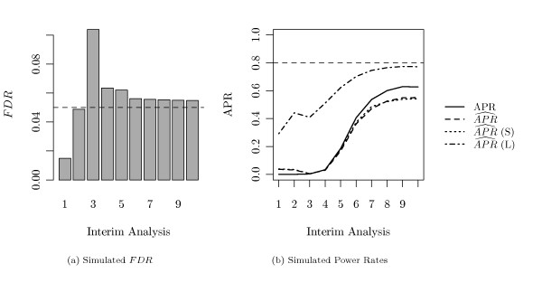
In the more extreme setting with only τ = 5% survival related genes, the overall course of the FDR over the interim analyses - as shown in Figure 6(a) and Table 3 - stays the same, but the peak in the early analyses becomes more prominent, and the specified FDR-level is not strictly maintained also during the later interim analyses.
Figure 6.
Simulated FDR and Power Rate (τ = 5%). The simulated FDR (a) and the real APR (solid line) with the APR estimates (broken lines) (b) at each interim analysis in the setting where 5% of all genes were altered between both groups.
Table 3.
Simulated FDR and Power Rate (10 Analyses τ = 5%)
| Analysis | ||||||||||
|---|---|---|---|---|---|---|---|---|---|---|
| 1 | 2 | 3 | 4 | 5 | ||||||
| mean | sd | mean | sd | mean | sd | mean | sd | mean | sd | |
| #found genes | 0 | 0 | 0 | 1 | 2 | 10 | 18 | 38 | 99 | 78 |
| FDR | 0.015 | 0.119 | 0.049 | 0.210 | 0.104 | 0.292 | 0.063 | 0.170 | 0.062 | 0.091 |
| APR | 0.000 | 0.000 | 0.000 | 0.001 | 0.003 | 0.019 | 0.033 | 0.070 | 0.185 | 0.146 |
 |
0.036 | 0.038 | 0.032 | 0.067 | 0.004 | 0.022 | 0.030 | 0.063 | 0.168 | 0.142 |
 (S) (S) |
0.038 | 0.047 | 0.034 | 0.090 | 0.005 | 0.030 | 0.032 | 0.082 | 0.177 | 0.182 |
 (L) (L) |
0.292 | 0.403 | 0.441 | 0.221 | 0.409 | 0.115 | 0.511 | 0.125 | 0.623 | 0.123 |
| 6 | 7 | 8 | 9 | 10 | ||||||
| mean | sd | mean | sd | mean | sd | mean | sd | mean | sd | |
| #found genes | 215 | 70 | 284 | 49 | 318 | 38 | 333 | 31 | 332 | 27 |
| FDR | 0.056 | 0.030 | 0.056 | 0.017 | 0.055 | 0.015 | 0.055 | 0.014 | 0.055 | 0.014 |
| APR | 0.406 | 0.132 | 0.537 | 0.092 | 0.601 | 0.070 | 0.629 | 0.058 | 0.627 | 0.049 |
 |
0.362 | 0.152 | 0.471 | 0.139 | 0.526 | 0.142 | 0.549 | 0.147 | 0.551 | 0.153 |
 (S) (S) |
0.373 | 0.220 | 0.486 | 0.224 | 0.522 | 0.215 | 0.539 | 0.217 | 0.543 | 0.221 |
 (L) (L) |
0.702 | 0.119 | 0.746 | 0.114 | 0.765 | 0.109 | 0.774 | 0.113 | 0.772 | 0.113 |
The descriptive values for each interim analysis including the number detected genes, the simulated FDR, the real APR, and the APR estimates, all in the setting of τ = 5% altered genes and ten interim analyses.
Average Power Rate and Early Stopping
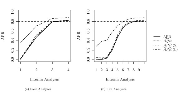
In Figure 5, the estimated and true APR at each interim analysis is shown. The corresponding descriptive values can be found in Tables 1 and 2. Again, the cases of M = 4 and M = 10 analyses are displayed, where half of the analyses took place during the recruitment part of the study and the other half during the follow-up part. In both cases, the estimated and the true APR increases with each interim analysis. In addition, true and estimated power do not diverge dramatically, however our estimation ( ) appears to be slightly liberal. Comparable performs the estimator
  (S), where we plug in the π0 estimation procedure of Storey and Tibshirani [8]. The power estimation by Marot and Mayer [4] (
 (L)) overestimates the real power.
Figure 5.
Simulated Power Rate (τ = 50%). True (solid line) and estimated (broken lines) average power rates (APR) at each interim analysis in the setting where 50% of all genes were altered between both groups. (a) M = 4 analyses, (b) M = 10 analyses. The dashed line marks the pre-specified stopping criterion, i.e. an estimated APR of 80%.
The pre-specified stopping criterion, an estimated APR of 80%, is represented by the dashed line. At average, this criterion is achieved at the 3rd analysis in the case of M = 4 planned interim analyses, and at the 7th analysis in the case of M = 10 planned interim analyses. In addition, true and estimated APR become not much higher than the desired level of 80%. In particular, the power increases when new samples are included during the recruitment part, but nearly stagnates in the follow-up part, where survival data is up-dated only.
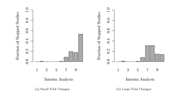
One main interest of our simulation was to find out whether interim analyses can provide an early stopping in such survival studies. Figure 7 shows for each interim analysis the fraction of simulation runs which could be stopped at this point. Both figures show the simulations with M = 10 analyses. The fold changes in these two settings were generated either with small effects (fold changes) or with large effects (compare Figure 3). In the case of small effects (Figure 7(a)), only 60% of all simulated studies reached the last planned final analysis while 40% were stopped at an interim analysis. In the case of large effects (Figure 7(b)), even more than 80% of the simulated studies were stopped before the final analysis.
Figure 7.
Simulated Stopped Studies (τ = 50%). Fractions of studies that could be stopped at each interim or at the final analysis in the setting where 50% of all genes were altered between both groups. (a) Case of small fold changes, (b) case of large fold changes between the genes of short and long time survivors.
The average power rate and its estimations in the harder setting with only τ = 5% survival related genes is shown in Figure 6(b). In this setting neither the true APR nor its estimates reach the 80% level, such that no study was stopped at earlier analyses. While the APR (L) again overestimates the true APR, the other estimators become conservative.
Application to Breast Cancer Data
In order to evaluate our method on real data, we analyzed gene expression levels from 295 patients suffering from breast cancer [9]. The data contain expression levels of 24496 genes. In this study, patients were recruited between 1984 and 1995. Thus, the recruitment part of the study was l1 = 11 years. Exact arrival times were not given in the public available data set, thus, we drew these times randomly from a uniform distribution U(0, l1). To account for random effects, which might have been introduced by drawing the arrival times, we repeated the simulated study based on this data 1000 times with newly drawn arrival times and took the average of the resulting error and power estimations.
In the data, minimum and maximum survival was 0.5 and 18 years, respectively. Median survival was 7 years. We analyzed the data set with M1 = 5 interim analyses during the recruitment part of the study and M2 = 5 analyses within the follow-up part. We intended to control the FDR at a level of 5% and to stop the study when the estimated APR exceeds 50%.
The raw p-values from the final analysis are displayed in Figure 2. From this figure it can be seen, that the suggested [8] choice of ϑ = 0.5 is indeed a good choice for this data, as the histogram resembles a uniform distribution very well in the range [0.5, 1].
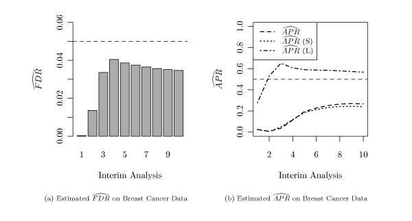
Figure 8 shows the estimated FDR and estimated APR at each interim analysis. The pre-specified FDR-level of 5% is not exceeded, and the estimated APR increases with each interim analysis. As in the simulation study, the estimator  (L) seems to overestimate the real APR. The estimators
  and
and  (S) again perform comparably. In the first interim analysis, no significant genes are detected. Thus,
  and
and  are equal zero. Interestingly, the stopping of an estimated 50%-APR is not achieved in any interim analysis when the more reliable APR estimators are used. In detail, the maximum achieved
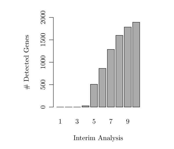
  was only 27% (with 1900 detected genes). Therefore, the study could not be stopped early with this criterion.
Figure 8.
Estimated Error and Power Rates on Real Data. Estimated FDR (a) and APR (b) at each interim analysis of the breast cancer data.
Figure 8(b) illustrates the different character of recruitment and follow-up part of the study. The increase of power is much stronger in the recruitment part than during the follow-up part, meaning that in this study not the available survival data but the sample size was the more restraining factor.
Simulation with Parameters from Breast Cancer Data
In order to perform the simulation also with different distributional assumptions, we performed an additional simulation, where parameters were taken from the breast cancer data described in the previous section. To this end we simulated the patient data and the gene expression data for 295 patients. Because the recruitment time of the real study was 11 years, the arrival times were again drawn randomly from a uniform distribution U(0, 11). A weibull, a gamma, and a log-normal distribution were fitted to the survival times of the real data using the fitdistcens function from the fitdistrplus R package [21]. We employed the Akaike Information Criterion (AIC) to select the fitted log-normal distribution, from which, thus, the survival times were drawn.
We wanted to set the proportion of survival related genes according to the real data set. We, therefore, used the results from the previous section where in the last analysis 1900 genes were found and the APR was estimated to be 27%. Thus, the total number of survival related genes in this data set was estimated to be 7037.
To generate the gene expression data, we divided the patients - as before - into two groups along their median survival time. The gene expression data was again multivariate normally distributed in both groups. The mean vector was set to 0 in one group. For the other group we used a discretization of the difference between the empirical mean vectors in both groups of the real data set. We chose the discretization grid to consist of steps with a width of 0.04, which resulted in 8542 survival related genes.
The distribution of the resulting mean vector of the second group is given in Table 4.
Table 4.
The Mean Gene Expression Vector in the Group of Long Time Survivors
| value | |||||||||||
| -0.24 | -0.2 | -0.16 | -0.12 | -0.08 | -0.04 | 0.00 | 0.04 | 0.08 | 0.12 | 0.16 | |
| # genes | 2 | 5 | 6 | 44 | 249 | 3336 | 15954 | 4507 | 335 | 50 | 8 |
In the simulation based on the parameters from the breast cancer data the mean vector of the gene expressions of the long time survivors is set to this discretized version of the difference of the empirical mean of the two groups in the real data.
We estimated the covariance matrix as proposed by Schäfer and Strimmer [22] using the implementation in the R package corpcor, but that resulted in a maximum power of 2.6% in the final analysis.
Therefore, we employed again a covariance matrix based on equation (12) as it was used in the other simulations. Because the effects in this simulation (see Table 4) were rather small, we reduced the simulated variance by a factor of 10 compared to the previous simulations.
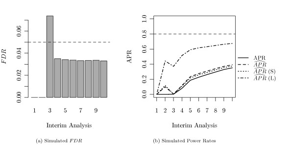
The results are shown in Figure 9 and Table 5. As in the simulation setting with τ = 5% survival related genes, the FDR peaks at the 3rd interim analysis, where only 14 genes were found on average. The APR estimators are comparable to the APR estimators in the real data, but show an erroneous aberration in the second analysis, even though there are no genes detected in that analysis. This aberration is corrected, though, in the third analysis as soon as there are some genes found.
Figure 9.
Simulated FDR and Power Rate (Parameters from the Breast Cancer Data). The simulated FDR (a) and the real APR (solid line) with the APR estimates (broken lines) (b) at each interim analysis in the simulation setting where parameters were taken from the breast cancer data.
Table 5.
Simulated FDR and Power Rates (Parameters from the Breast Cancer Data)
| Analysis | ||||||||||
|---|---|---|---|---|---|---|---|---|---|---|
| 1 | 2 | 3 | 4 | 5 | ||||||
| mean | sd | mean | sd | mean | sd | mean | sd | mean | sd | |
| #found genes | 0 | 0 | 0 | 0 | 14 | 34 | 701 | 227 | 1650 | 396 |
| FDR | 0.000 | 0.000 | 0.000 | 0.000 | 0.074 | 0.179 | 0.035 | 0.008 | 0.034 | 0.005 |
| APR | 0.000 | 0.000 | 0.000 | 0.000 | 0.002 | 0.004 | 0.079 | 0.026 | 0.186 | 0.045 |
 |
0.000 | 0.000 | 0.100 | 0.160 | 0.004 | 0.008 | 0.117 | 0.031 | 0.234 | 0.044 |
 (S) (S) |
0.000 | 0.000 | 0.118 | 0.238 | 0.003 | 0.007 | 0.107 | 0.029 | 0.217 | 0.043 |
 (L) (L) |
0.000 | 0.000 | 0.443 | 0.374 | 0.371 | 0.032 | 0.514 | 0.030 | 0.591 | 0.029 |
| 6 | 7 | 8 | 9 | 10 | ||||||
| mean | sd | mean | sd | mean | sd | mean | sd | mean | sd | |
| #found genes | 2005 | 413 | 2318 | 457 | 2614 | 442 | 2906 | 447 | 3107 | 439 |
| FDR | 0.034 | 0.005 | 0.033 | 0.005 | 0.033 | 0.005 | 0.034 | 0.004 | 0.033 | 0.004 |
| APR | 0.227 | 0.046 | 0.262 | 0.051 | 0.296 | 0.050 | 0.329 | 0.050 | 0.352 | 0.050 |
 |
0.275 | 0.046 | 0.308 | 0.050 | 0.341 | 0.048 | 0.371 | 0.048 | 0.392 | 0.046 |
 (S) (S) |
0.259 | 0.046 | 0.289 | 0.051 | 0.324 | 0.049 | 0.354 | 0.050 | 0.375 | 0.051 |
 (L) (L) |
0.617 | 0.029 | 0.631 | 0.029 | 0.648 | 0.029 | 0.664 | 0.030 | 0.675 | 0.032 |
The descriptive values for each interim analysis including the number detected genes, the simulated FDR, the real APR, and the APR estimates, all in the setting where parameters were taken from the breast cancer data.
Discussion
Typically, survival studies require long time spans from recruitment of the first patients until the availability of first results. Therefore, there is a strong desire to obtain results prior to the planned end of the study, not only for financial aspects but also for ethical ones. Classical group sequential designs exhibit a methodology for interim analyses including the potential for an early stopping of a trial. Whereas these classical methods concentrate on studies with one single feature, there has little been done for the case of multiple features, particularly the high-dimensional case. However, many survival studies now concentrate on correlating observed survival times with high-throughput data from genomics or proteomics experiments which yield expression levels for thousands of features measured in a small number of samples.
Based on the findings of Marot and Mayer [4] and Posch et al. [5] we simulated the possibility of early stopping in interim analyses of survival data in microarray experiments. Likewise to these prior findings we observed that a pre-specified false discovery rate is maintained during interim analyses without particular adjustments. I.e., adjustment appears only to be necessary for multiple testing but not additionally for interim analysis. While it was shown in the two mentioned articles that this principle holds asymptotically when the number of tested hypothesis is large, we have seen in further simulations beyond those presented in the section on the simulation that it also works for rather small numbers of hypotheses (e.g. testing 500 genes).
We used the Benjamini-Hochberg procedure to do the multiple testing adjustment, even though the Benjamini-Hochberg procedure does not control the FDR under arbitrary dependency structures. However, in our simulations and in the real data example it could be seen that this procedure mostly controlled the FDR. We believe, that in microarray studies a strict control of the FDR is of minor importance, as microarray studies are mainly used for hypothesis generation and, thus, need further validation anyway. In cases where a stricter control of the FDR is required, the more conservative procedure of Benjamini and Yekutieli [23] might be more appropriate.
An important issue in interim analyses of high-dimensional data is the choice of an adequate stopping criterion. Here, we chose the achieved average power rate as stopping criterion which is defined as the proportion of detected false null hypothesis. We derived a new estimator for the average power rate that comes close to the true proportion of true positive findings. However, this estimator behaved slightly liberal when the data contained many survival related genes and conservative when the data contained few survival related genes. We also tried other methods like the more sophisticated ϑ estimator given in [8] and the APR estimation method proposed in [4] which resulted in comparable and worse approximations, respectively. Improvements remain therefore necessary. With this criterion we observed that early stopping can be achieved in certain studies, based on the actual proportion of false null hypothesis and the effect sizes (size of fold changes).
We applied the methods onto gene expression data from a microarray study on breast cancer. In this analysis we obtained an estimated average power of 20% at the fifth interim analysis (i.e. roughly five years after begin of the study) and of 27% at the eighth interim analysis (i.e., roughly after eight years). These estimated proportions seem to be rather small. However, the estimated APR of 27% in the final analysis corresponds to about 1900 genes detected by Cox regression (see Figure 10). This set might provide a signature which enables to build a survival predictor of sufficient quality. Predictor quality and classification accuracy are other interesting stopping criteria for interim analyses of high-dimensional data. The prognostic value of survival models based on gene expression signatures was for example studied by Hielscher et al. [24]. Evaluation of such alternative stopping criteria remains an open point which we are going to study in our further research.
Figure 10.
Number of Significant Genes in Real Data. Number of detected survival related genes at each interim analysis of the breast cancer data.
The necessary sample size another important point in planning microarray studies in combination with survival data. Our simulation study provides the basis for such sample size considerations. With certain information from pilot studies, including expected distributions of fold changes and expected survival times, our simulation approach can be used to study the development of the APR in interim analyses. Therefore, we made our R-code available as package on the R-CRAN repository http://cran.r-project.org within the package survGenesInterim.
Several extensions of our simulation framework can be considered. In the analysis of microarray experiments normalization is an important pre-processing step to make the single arrays comparable. We therefore intent as methodological improvement to add different normalization approaches to our simulation framework. When making interim analyses, one can for example consider a re-normalization with each set of new array data or use the normalization parameters obtained in a previous interim analysis. Another improvement can be considered with regard to the survival analysis. While we have used the proportional hazard model, here, this assumptions may not always be true and other models with time variant effects seem to be more reliable.
Conclusions
Group sequential interim analyses of microarray experiments in survival studies are frequently performed without considering the adherence of the overall error rate. Our simulation framework helps to evaluate the behaviour of error rates and power rates in such experiments. The framework also enables to study the developing of results when survival data is up-dated at subsequent times during studies that take several years.
Authors' contributions
KJ formulated the problem and the study design. AL wrote the R-code and performed the simulations and the data evaluation. TB provided important contributions concerning the practical aspects of the study design. All authors were involved in writing the manuscript and have read and approved the final manuscript.
Contributor Information
Andreas Leha, Email: Andreas.Leha@med.uni-goettingen.de.
Tim Beißbarth, Email: tim.beissbarth@med.uni-goettingen.de.
Klaus Jung, Email: Klaus.Jung@ams.med.uni-goettingen.de.
Acknowledgements
This work was supported by the Deutsche Forschungsgemeinschaft (KFO 179) and by the German Federal Ministry of Education and Research (BMBF) within the NGFN network IG Prostate-Cancer(01GS0890) and within the Medical Systems Biology network BreastSys. We thank the reviewers for their constructive comments.
References
- Pocock SJ. Group sequential methods in the design and analysis of clinical trials. Biometrika. 1977;64(2):191–199. doi: 10.1093/biomet/64.2.191. [DOI] [Google Scholar]
- O'Brien PC, Fleming TR. A multiple testing procedure for clinical trials. Biometrics. 1979;35(3):549–556. doi: 10.2307/2530245. [DOI] [PubMed] [Google Scholar]
- Armitage P, McPherson CK, Rowe BC. Repeated Significance Tests on Accumulating Data. Journal of the Royal Statistical Society. Series A (General) 1969;132(2):235–244. doi: 10.2307/2343787. [DOI] [Google Scholar]
- Marot G, Mayer CD. Sequential Analysis for Microarray Data Based on Sensitivity and Meta-Analysis. Statistical Applications in Genetics and Molecular Biology. 2009;8(1,3) doi: 10.2202/1544-6115.1368. [DOI] [PubMed] [Google Scholar]
- Posch M, Zehetmayer S, Bauer P. Hunting for Significance With the False Discovery Rate. Journal of the American Statistical Association. 2009;104(486):832–840. doi: 10.1198/jasa.2009.0137. [DOI] [Google Scholar]
- Cox DR. Regression Models and Life-Tables. Journal of the Royal Statistical Society. Series B (Methodological) 1972;34(2):187–220. [Google Scholar]
- Victor A, Hommel G. Combining Adaptive Designs with Control of the False Discovery Rate - A Generalized Definition for a Global p-Value. Biometrical Journal. 2007;49:94–106. doi: 10.1002/bimj.200510311. [DOI] [PubMed] [Google Scholar]
- Storey JD, Tibshirani R. Statistical significance for genomewide studies. Proceedings of the National Academy of Sciences of the United States of America. 2003;100(16):9440–9445. doi: 10.1073/pnas.1530509100. [DOI] [PMC free article] [PubMed] [Google Scholar]
- van de Vijver MJ, He YD, van't Veer LJ, Dai H, Hart AA, Voskuil DW, Schreiber GJ, Peterse JL, Roberts C, Marton MJ, Parrish M, Atsma D, Witteveen A, Glas A, Delahaye L, van der Velde T, Bartelink H, Rodenhuis S, Rutgers ET, Friend SH, Bernards R. A gene-expression signature as a predictor of survival in breast cancer. New England Journal of Medicine. 2002;347(25):1999–2009. doi: 10.1056/NEJMoa021967. [DOI] [PubMed] [Google Scholar]
- Simon R, Korn E, McShane L, Radmacher M, Wright G, Zhao Y. Design and Analysis of DNA Microarray Investigations. chap 7.8. Springer New York. Statistics for Biology and Health; 2004. [Google Scholar]
- Altman DG. Practical Statistics for Medical Research. chap 13. Chapman & Hall/CRC; 2006. [Google Scholar]
- Therneau TM, Grambsch PM. Modeling Survival Data: Extending the Cox Model (Statistics for Biology and Health) 1. Springer, Berlin; 2000. 2nd printing edition 2001. [Google Scholar]
- Park PJ, Tian L, Kohane IS. Linking gene expression data with patient survival times using partial least squares. Bioinformatics. 2002;18(Suppl 1):S120–7. doi: 10.1093/bioinformatics/18.suppl_1.s120. [DOI] [PubMed] [Google Scholar]
- Dudoit S, Shaffer JP, Boldrick JC. Multiple Hypothesis Testing in Microarray Experiments. Statistical Science. 2003;18:71–103. doi: 10.1214/ss/1056397487. [DOI] [Google Scholar]
- Benjamini Y, Hochberg Y. Controlling the false discovery rate: A practical and powerful approach to multiple testing. Journal of the Royal Statistical Society: Series B (Statistical Methodology) 1995;57:289–300. [Google Scholar]
- Storey JD, Taylor JE, Siegmund D. Strong control, conservative point estimation and simultaneous conservative consistency of false discovery rates: a unified approach. Journal Of The Royal Statistical Society Series B. 2004;66:187–205. doi: 10.1111/j.1467-9868.2004.00439.x. [DOI] [Google Scholar]
- Storey JD. A direct approach to false discovery rates. Journal of the Royal Statistical Society: Series B (Statistical Methodology) 2002;64(3):479–498. doi: 10.1111/1467-9868.00346. [DOI] [Google Scholar]
- Langaas M, Lindqvist BH, Ferkingstad E. Estimating the proportion of true null hypotheses, with application to DNA microarray data. Journal Of The Royal Statistical Society Series B. 2005;67(4):555–572. doi: 10.1111/j.1467-9868.2005.00515.x. [DOI] [Google Scholar]
- Pounds S, Morris SW. Estimating the occurrence of false positives and false negatives in microarray studies by approximating and partitioning the empirical distribution of p-values. Bioinformatics. 2003;19(10):1236–42. doi: 10.1093/bioinformatics/btg148. [DOI] [PubMed] [Google Scholar]
- R Development Core Team. R: A Language and Environment for Statistical Computing. R Foundation for Statistical Computing, Vienna, Austria; 2010. http://www.R-project.org [ISBN 3-900051-07-0] [Google Scholar]
- Delignette-Muller ML, Pouillot R, Denis JB, Dutang C. fitdistrplus: help to fit of a parametric distribution to non-censored or censored data. 2010. [R package version 0.1-3]
- Schäfer J, Strimmer K. A shrinkage approach to large-scale covariance matrix estimation and implications for functional genomics. Stat Appl Genet Mol Biol. 2005;4:Article32. doi: 10.2202/1544-6115.1175. [DOI] [PubMed] [Google Scholar]
- Benjamini Y, Yekutieli D. False Discovery Rate-Adjusted Multiple Confidence Intervals for Selected Parameters. Journal of the American Statistical Association. 2005;100(469):71–81. doi: 10.1198/016214504000001907. [DOI] [Google Scholar]
- Hielscher T, Zucknick M, Werft W, Benner A. On the prognostic value of survival models with application to gene expression signatures. Stat Med. 2010;29(7-8):818–29. doi: 10.1002/sim.3768. [DOI] [PubMed] [Google Scholar]


