Estimator for photon counting energy selective x-ray imaging with multibin pulse height analysis

Abstract

Purpose: This paper describes a noniterative estimator for the energy dependent information from photon counting detectors with multibin pulse height analysis (PHA). The estimator uses the two function decomposition of the attenuation coefficient [R. E. Alvarez and A. Macovski, Phys. Med. Biol. 21, 733–744 (1976)] and its output is the line integrals of the basis set coefficients. The output noise variance and bias is compared to other noniterative estimators and to the Cramèr-Rao lower bound (CRLB).

Methods: The estimator first computes an initial estimate from a linearized maximum likelihood estimator. The errors in the initial estimates are determined at a set of points from measurements on a calibration phantom. The errors at these known points are interpolated to create two-dimensional look up tables of corrections to the initial estimates. During image acquisition, the linearized maximum likelihood estimate for each data point is used as an input to the correction look up tables, and the final output is the sum of the estimate and the correction. The performance of the estimator is compared to generalizations of the polynomial and rational polynomial estimators for multibin data. The estimators are compared by the mean square error (MSE) and its components, the bias, and the variance of the output. The variance is also compared to the CRLB. The performance is simulated with two to five bins PHA data. The CRLB at a fixed object thickness is also computed as a function of the number of bins.

Results: For two bin data, all the estimators’ variances are equal to the CRLB. With three or more bins, only the proposed estimator achieves the CRLB while the others, which were not optimized for noise performance, have much larger output variance. The bias of the proposed estimator is equal to the polynomial estimator for calibration phantoms with 40 or more steps, that is, 1600 combinations of basis materials, but is larger than the rational polynomial bias. In all cases at the photon counts tested, the MSE is essentially equal to the variance, indicating that the bias errors are negligible compared to the variance.

Conclusions: The estimator provides a noniterative method to compute the energy dependent information from multibin PHA data that achieves the CRLB over a wide range of operating conditions and has low output bias. The estimator can be calibrated based on the measurements of a calibration phantom; so, it does not require measurements of the x-ray energy spectrum or the detector response functions.

INTRODUCTION

One of the principal reasons for the interest in photon counting detectors for medical x-ray imaging is their ability to extract energy spectrum information through pulse height analysis (PHA).¹ These detectors can analyze the photons into two or more energy bins but most prior research on solving the equations for the energy dependent information² assumed only two effective spectra.^{3, 4, 5, 6, 7} In this paper, I describe an estimator for multibin PHA data and show that its output noise variance is equal to the Cramèr-Rao lower bound (CRLB) (Refs. ^{8, 9}) over a wide range of operating conditions. Since the estimator achieves the CRLB, we can be assured that no other unbiased estimator has a smaller noise variance. Other advantages of the estimator include that it can be calibrated based on transmission data of a calibration phantom with the x-ray system; so, it does not require measurements of the x-ray energy spectrum or the detector response functions. Also, the estimator is noniterative; so, it can be computed rapidly with a fixed maximum computation time.

Prior research on estimators for the energy dependent information^{3, 4, 5, 6, 7} emphasized deterministic errors with a low noise data and computation time. While these errors are important, they are only part of a broader measure of performance that is widely used in estimator theory, the mean square error (MSE). The MSE is the expected value of the square of the difference of the output and the actual value and is equal to the sum of the variance and the square of the bias (see Sec. 2.4 of Kay⁸). The bias is the difference of the expected value of the output and the actual value while the variance is the expected value of the square of the difference of the output and its mean value. The deterministic errors correspond to the bias, but in medical imaging systems, the variance can be significantly larger than the square of the bias; so, both are measured in this paper. Prior noniterative methods such as the polynomial and rational polynomial³ estimators can be generalized for more than two spectra but, since they were not designed to take into account the noise properties, their output noise variance with multibin data is much larger than the proposed estimator. The proposed estimator has comparable bias to the polynomial and rational polynomial estimators so it has a much smaller MSE.

The maximum likelihood approach (see Sec. 2.4 of Van Trees⁹ and Chap. 7 of Kay⁸) can be applied with multibin PHA data to produce estimators with desirable characteristics including being asymptotically unbiased and efficient, i.e., with output variance equal to the CRLB. However, as previously implemented, maximum likelihood estimators (MLE) require an iterative maximization with the data at each pixel or CT scanner channel. For example, Roessl and Proksa¹⁰ discuss the theory of an iterative MLE for multibin PHA data, and Schlomka et al.¹¹ describe its experimental implementation. While this is impressive work, their method has substantial problems for clinical utilization. One problem is computation. Iterative methods can potentially fail to converge and have long, unpredictable computation times. Another problem is that the method by Roessl and Proksa and Schlomka et al. requires knowledge of the incident energy spectrum at high resolution and the effective energy response of each bin. This is problematic for clinical installations since, due to aging of components, the sputtering of anode material on the x-ray tube window, and other effects, the spectra and detector response may change and must be measured periodically. The measurements required for the iterative algorithm use specialized instruments and techniques and would be difficult to carry out in a clinical environment.

An alternative is to estimate the spectrum from transmission measurements.^{5, 6} However, it is unclear whether the reconstructed spectra are sufficiently accurate. Indeed, the spectrum reconstruction methods were suggested principally for objects that are too large or too small for practical construction of a calibration phantom. The method described here is based directly on calibration phantom measurements without the intermediate step of estimating the spectrum.

I compare the performance of the estimator to generalizations of the polynomial and rational polynomial approximations for multibin data. The performance is measured using a Monte Carlo simulation. The estimators are compared by the bias, the variance, and the MSE of the output with noisy data. The variance is also compared to the CRLB. The performance is simulated for detectors with two to five bins PHA.

METHODS

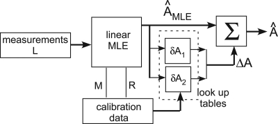
The operation of the proposed estimator is shown in Fig. 1. The estimator uses the two function decomposition of the x-ray attenuation coefficient² and its output is the line integrals of the basis set coefficients. These line integrals can be considered to be the components of a two-dimensional vector, A, called the A-vector here, and the output for each pixel or CT scanner channel is a point in a two-dimensional space, called the A-plane. Since the two function decomposition accurately approximates the attenuation coefficient if the material has no K-edges within the energy region of interest, the A-plane data completely characterize the information that can be extracted by an x-ray imaging system.

Figure 1.

The A-table estimator block diagram. See text for the definitions of the measurement data vector L, the transfer matrix M, and the covariance R as well as for a description of the operation.

The first step in the estimator is to compute an initial estimate based on a linearized MLE. This transforms the detector data to the two-dimensional A-plane regardless of the number of bins in the PHA. The initial estimate can be implemented as a matrix multiplication so it can be computed rapidly without iteration. Since the x-ray transmission is a nonlinear function of A, the initial estimate will have errors. In the second step, the errors in the two components of the A-vector are corrected using data from two-dimensional look up tables that are computed based on measurements with a calibration phantom using the imaging system x-ray source and detectors. Since the estimator uses look up tables with A-vectors as inputs, it will be referred to as the A-table estimator.

In this section, the initial estimator is first derived. Next, a calibration phantom that can be used to provide data to compute the estimator parameters is described. I then show how the calibration phantom data can be used to compute the initial estimator parameters and the correction look up tables. The variance will be compared with the CRLB, so I derive an expression for the CRLB variances in terms of the system parameters. I then describe generalizations of the polynomial and rational polynomial estimators for more than two effective spectra and methods to compute the parameters of these estimators from the calibration phantom data. Finally, I describe the methods to measure the performance of the estimators based on Monte Carlo simulator data.

A linearized MLE

The purpose of the initial estimator is to provide A-plane data that are close enough to the noise-optimal estimate so that the corrections applied from the look up tables can provide accurate, near noise-optimal, results. The initial estimator is based on a linearized MLE with some modifications as noted below. The performance of the complete A-table estimator is determined by the interaction of the initial estimator and the correction factors.

The derivation of the initial estimator is based on a linearized model of the multibin PHA measurements. The model uses the two function decomposition² of the x-ray attenuation coefficient, which is applicable with lower atomic number materials without K-edges in the diagnostic energy region. This method is well-known but will be described here to introduce notation. The attenuation coefficient μ(r,E) at each point r in the object at photon energy E can be decomposed as,

$\mu (\mathbf{r},E)=a_1(\mathbf{r})f_1(E)+a_2(\mathbf{r})f_2(E)$

where a₁(r) and a₂(r) are the basis set coefficients and f₁(E) and f₂(E) are the basis functions. Since the basis functions are known a priori, all the information is carried by the basis set coefficients. We cannot measure these coefficients directly. Instead, we infer them from measurements of the transmitted flux through the object with two or more source spectra. The x-ray source, typically an x-ray tube, produces photons with an energy spectrum s_source(E), which can be either the photon number spectrum n(E) or the photon energy spectrum q(E) = En(E) depending on the type of detector used. The detector area and the exposure time are assumed to be included in the spectrum values. The spectrum of the x-ray photons transmitted through the object is

$$s_{\mathrm{Trans}}(E)=s_{\mathrm{source}}(E)e^{-\int \mu (\mathbf{r},E)\mathit{dt}},$$ (1)

where ∫μ(r,E)dtdt is the line integral of the attenuation coefficient on a line from the x-ray tube focal spot to the detector. Using the basis set decomposition, the line integral can be expressed as

$$\int \mu (\mathbf{r},E)\mathit{dt}=A_1{f}_1(E)+A_2{f}_2(E),$$ (3)

where A_i=∫a_i(r)dt, i = 1,2. The line integrals A₁ and A₂ will be considered to be the components of a vector A. The x-ray imaging system can then be considered to map the object x-ray attenuation onto a set of points in an abstract two-dimensional vector space, the A-plane.

The PHA detector analyzes the energy of individual photons and counts the number that fall within a set of energy bins during the exposure time. The mean values of the counts N_k are the integrals of the spectrum of the photons incident on the detector times the effective response function of the bin d_k(E). In an idealized model, d_k(E) is a rectangle function that is one inside the bin and zero outside but it can also model other responses. Using (1), the mean values are

$$N_k=\int d_k(E)n_{\mathrm{source}}(E)e^{-\int \mu (\mathbf{r},E)\mathit{dt}}\mathit{dE}.$$ (3)

Substituting the expression for the line integral (2), we can see that the counts are functions of the A-vector

$$N_k(\mathbf{A})=\int d_k(E)n_{\mathrm{source}}(E)e^{-A_1{f}_1(E)-A_2{f}_2(E)}\mathit{dE}.$$ (4)

The measurements will be summarized as components of a vector I. Because of the exponential form of the transmission equations [Eq. 1], the logarithms of the measurements L = −log(I∕I₀) can approximately linearize them, where the components of I₀ are the expected values with no object in the beam. The negative is used to give positive quantities since the measurements decrease with increasing object thickness.

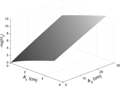
From (4), we see that the vector L is a function of A. Figure 2 shows the near linearity of L(A).

Figure 2.

Three-dimensional plot of L as a function of A for data from a single bin. Note that L is approximately linear. There are comparable plots for the logarithm of data from other bins.

To derive a linearized model, we can use a vector Taylor’s series expansion of L(A) about a mean value $\stackrel{-}{\mathbf{A}}$

$$\mathbf{L}(\stackrel{-}{\mathbf{A}}+\delta \mathbf{A})=\mathbf{L}(\stackrel{-}{\mathbf{A}})+\frac{\partial \mathbf{L}}{\partial \mathbf{A}}\delta \mathbf{A}+\dots .$$ (5)

Expanding about the origin, where $\stackrel{-}{\mathbf{A}}=0$, and noting that, by definition, L(0) = 0, we can drop the higher order terms to obtain a linear model

$$\mathbf{L}(\mathbf{A})\approx \frac{\partial \mathbf{L}}{\partial \mathbf{A}}\mathbf{A},$$ (6)

where the gradient ∂L∕∂A is evaluated at the origin. The gradient is a matrix M with coefficients

$$M_{\mathit{ij}}=-\frac{\partial \mathit{log}(I_i∕I_{i0})}{\partial A_j}=-\frac{1}{I_i}\frac{\partial I_i}{\partial A_j}.$$

Substituting the integral expression for the measurements

$$M_{\mathit{ij}}=\frac{\int f_j(E)d_i(E)s_i(E)e^{-A_1{f}_1(E)-A_2{f}_2(E)}\mathit{dE}}{\int d_i(E)s_i(E)e^{-A_1{f}_1(E)-A_2{f}_2(E)}\mathit{dE}}.$$

Defining the normalized spectrum

$${\stackrel{\wedge }{s}}_i(E)=\frac{d_i(E)s_i(E)e^{-A_1{f}_1(E)-A_2{f}_2(E)}}{\int d_i(E)s_i(E)e^{-A_1{f}_1(E)-A_2{f}_2(E)}\mathit{dE}},$$ (7)

$$M_{\mathit{ij}}=\int f_j(E){\stackrel{\wedge }{s}}_i(E)\mathit{dE}={〈f_j(E)〉}_i.$$ (8)

That is, the coefficients of the M matrix are the average or effective values of the basis set functions over the normalized spectra ${\stackrel{\wedge }{s}}_i(E)$. The number of rows of M is equal to the number of spectra or bins in a PHA detector and it has two columns, one for each component of the A-vector.

The MLE requires a probabilistic model for the L measurement data and I will use a multivariate normal distribution, which is widely used to model x-ray imaging system data.¹² Then, the linear model with noise is

$${\mathbf{L}}_{\mathrm{with}\mathrm{}\mathrm{noise}}(\mathbf{A})=\mathbf{MA}+\mathbf{w},$$ (9)

where w is a zero mean multivariate normal random variable whose covariance depends on A.

The MLE for this linearized system is derived in standard textbooks [see Eq. 4 of Kay⁸]

$${\stackrel{\wedge }{\mathbf{A}}}_{\mathrm{MLE}}=({\mathbf{M}}^T{\mathbf{R}}_{L|A}^{-1}\mathbf{M}){}^{-1}{\mathbf{M}}^{\mathbf{T}}{\mathbf{R}}_{\mathbf{L}|\mathbf{A}}^{-1}{\mathbf{L}}_{\mathrm{with}\mathrm{}\mathrm{noise}}.$$ (10)

where R_L|A is the covariance of the L data. The matrices M and R_L|A are determined from the calibration data as shown in Secs. 2B, 2C so that the leading factor of Eq. 10, $({\mathbf{M}}^T{\mathbf{R}}_{L|A}^{-1}\mathbf{M}){}^{-1}{\mathbf{M}}^{\mathbf{T}}{\mathbf{R}}_{\mathbf{L}|\mathbf{A}}^{-1}$, can be precomputed resulting in a single matrix. The initial estimate is therefore a matrix multiplication times the measurement vector L_with noise so it can be computed rapidly.

The calibration phantom

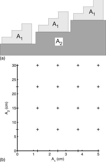
The initial estimator parameters and the correction look up tables can be computed from measurements with the calibration phantom shown in Fig. 3a. The phantom is made from step wedges with accurately known dimensions and made of materials, such as acrylic plastic and aluminum, whose chemical composition spans the range of atomic numbers of materials found in the object. The maximum thicknesses of the step wedges are chosen to span the attenuation of the subjects. For the simulations, these were chosen to be 5 cm of aluminum and 30 cm of acrylic plastic. The phantom can be placed in the imaging system and measurements made using the same x-ray technique as would be used for the object. In a CT system, the gantry would be fixed to make measurements of the projections of the phantom. If the responses of the channels are substantially different, the phantom could be constructed wide enough to fit over all the channels and scanned across the detector so the data are measured for each channel. The calibration data could then be used to compute MLE parameters and correction look up tables for individual channels. The scanning procedure and the extraction of the measurements from the system data can be automated and done under software control.

Figure 3.

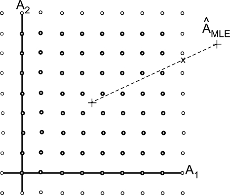
Calibration phantom. (a) Two sets of step wedge phantoms made from known materials and with equal increments are used. The measurements provided data at points on a rectangular lattice on the A-plane are shown in (b).

If we use the calibration material basis set¹³ so the basis functions f₁(E) and f₂(E) are the attenuation coefficients of the step wedge materials, then the A-vector components are the thicknesses of each type of material in the phantom. As a result, we can sort the calibration phantom data to give the measurement vector L at a rectangular lattice of points on the A-plane shown in Fig. 3b.

Linear MLE parameters from calibration phantom data

Equation 10 gives the estimated ${\stackrel{\wedge }{\mathbf{A}}}_{\mathbf{MLE}}$ for a given measured data vector L. Its evaluation requires the effective attenuation coefficient matrix M and the covariance matrix R. These can be computed from the calibration phantom data.

The effective attenuation coefficient matrix M is approximated as the coefficients of a least squares regression of L as a function of A with the calibration data. In the linearized model (6), M is the gradient at the origin but, for the implementation of the MLE, I use the average over the calibration data

$${\mathbf{L}}_{\mathrm{calibration}}={\mathbf{MA}}_{\mathrm{calibration}}.$$ (11)

The matrices L_calibration and A_calibration are measured with the calibration phantom and we can use least squares to find the coefficients M that are the best fit to the data. This will give an average value of M over the complete phantom but, since the linear MLE will be used as an initial estimate, this gives sufficient accuracy.

The covariance can be computed from measurements on a uniform region of the step wedge so all the measurements are samples of the random data for a constant A-vector. The sample covariance will then be an estimate of R. Even though the expansion in Eq. 6 is about the origin, I found that better results were obtained by using the covariance from the center of the calibration region, 2.5 cm of aluminum and 15 cm of acrylic plastic. Thus, the computation of both the gradient M and the covariance R do not precisely use the linearized model of Eq. 6. However, when used with the correction table discussed in Sec. 2D , the overall estimator produces small errors.

The correction look up table

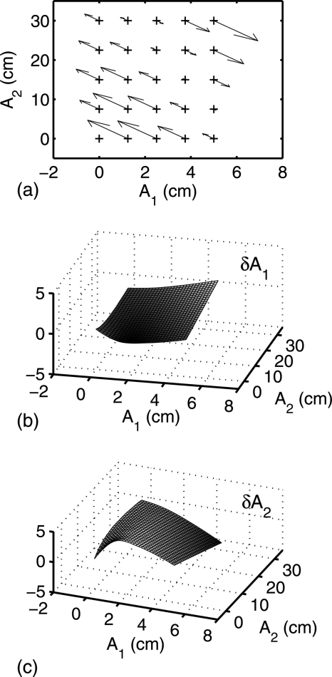
We can also use the calibration phantom data to compute the error correction look up tables. Since the overall mapping from L to A is nonlinear, we expect the linearized MLE to produce errors. The calibration data give us the actual values of the A-vectors for the L data at the grid of A-plane points in Fig. 3b. By subtracting the actual A values from the linear MLE outputs at these points, we can compute the errors. Figure 4a shows the errors as arrows from the actual values to the initial estimates.

Figure 4.

Initial estimator errors. Part (a) shows the errors derived from the calibration phantom data. Parts (b) and (c) show the corrections for each of the A-vector components as a function of the initial values ${\stackrel{\wedge }{\mathbf{A}}}_{\mathrm{intial}}$.

As shown in Figs. 4b, 4c, the errors are smooth two-dimensional functions for each A-vector component. We can use the smoothness of these functions to compute a two-dimensional look up table by interpolating between the values determined from the calibration phantom data.

The inputs to the correction look up tables are the outputs of the initial estimator, that is, the arrow heads in Fig. 4a. They are, therefore, not on a rectangular lattice. However, we can use the MATLABgridfit function¹⁴ or similar techniques to interpolate them onto a rectangular lattice suitable for the look up tables. The gridfit function interpolates between nonuniformly spaced points by solving a set of simultaneous equations for the parameters of a hypothetical flexible plate that approximates the data. By using this function, we can compute a high-resolution, rectangular look up table that can be used for fast computation of the corrections from individual measurements during the operation of the system.

Due to random noise fluctuations, it is possible, although improbable, for the initial estimator output to be outside the region of the A-plane covered by the look up tables. This can be dealt with in two ways. The first is to use the extrapolation capability of the gridfit function to expand the region of coverage. The function’s algorithm allows the calibration data to be extrapolated smoothly for small regions outside the region with data. I expanded the calibration region by 20% about its centroid. Data that fall outside this region were assigned the calibration table values on the nearest boundary on a line joining the point and the calibration table centroid, as shown in Fig. 5.

Figure 5.

Algorithm for data that fall outside calibration region. The calibration table is extrapolated using the gridfit function as shown by the light circles. For data that are outside this region, the table value at the nearest boundary on a line joining the point and data centroid is used. This is the point marked with the X.

The accuracy of the estimator depends on the spacing between the calibration points and therefore on the number of steps in the step wedges. This accuracy is studied using the Monte Carlo simulation as described in Sec. 2G.

The CRLB

The performance of the estimators was compared to the CRLB. As discussed in Sec. 2I, this is a lower limit for the variance of any unbiased estimator. Estimators that achieve the CRLB are called “efficient.” In our case, the covariance of the noise in Eq. 9 depends on the estimated parameters. The CRLB in this general normal case is derived in Sec. 3.9 of Kay.⁸ It is the inverse of the Fisher information matrixF whose elements are given by Eq. (3.31) of this reference.

Translating this equation to our notation, the elements of the matrix are

$$\begin{array}{c}\multicolumn{1}{c}{[\mathbf{F}(\mathbf{A})]{}_{\mathit{ij}}=\mathbf{M}(:,i){}^T{\mathbf{R}}^{-1}\mathbf{M}(:,j)+\frac{1}{2}\mathit{tr}\left[{\mathbf{R}}^{-1}\frac{\partial \mathbf{R}}{\partial {\mathbf{A}}_{\mathbf{i}}}{\mathbf{R}}^{-1}\frac{\partial \mathbf{R}}{\partial {\mathbf{A}}_{\mathbf{j}}}\right],}\end{array}$$ (12)

where M(:, i) is column i of M and tr[] is the trace of the matrix in the brackets.

The CRLB will depend on the point in the A plane so that the matrices in (12) need to be evaluated for the specified point. We can use the normalized transmitted spectrum Eq. 7 with Eq. 8 to compute M. The covariance matrix of the logarithm of the photon counts is derived in my previous paper¹⁵

$$\mathbf{R}=\left[\begin{array}{ccc}\multicolumn{1}{c}{1∕N_1}& \hfill \hfill & \hfill \hfill \\ \multicolumn{1}{c}{}& \hfill \hfill & \hfill \hfill \\ \multicolumn{1}{c}{}& \hfill \hfill & \hfill 1∕N_K\hfill \end{array}\right].$$

In this equation, N_k is the parameter of the Poisson distribution of the counts of bin k and can be computed for a specified A-vector using Eq. 18. To complete the evaluation of F(A), we also need the derivative ∂R∕∂A_i. This is the derivative of each element of R with respect to the scalar A_i. Since R is diagonal, we only need the derivative of each diagonal element

$$\frac{\partial }{\partial {\mathbf{A}}_{\mathbf{i}}}\left(\frac{1}{N_k}\right)=-\frac{1}{N_k^2}\frac{\partial N_k}{\partial A_i}=-\frac{M_{\mathit{ki}}}{N_k},$$ (13)

which can be computed at each point from M and N_k.

Polynomial and rational polynomial estimators

We can derive estimators by generalizing methods discussed in the literature for the two spectra. One method that is widely used is a polynomial approximation to the inverse transformation. With two spectra, the second order approximation is

$$A_1=c_0+c_1{L}_1+c_2{L}_2+c_3{L}_1^2+c_4{L}_1{L}_2+c_5{L}_2^2,$$ (14)

$$A_2=d_0+d_1{L}_1+d_2{L}_2+d_3{L}_1^2+d_4{L}_1{L}_2+d_5{L}_2^2,$$ (15)

where L_k = −log(I_k∕I_k0), k = 1,2. The equations are linear in the coefficients so that they can be determined with a least squares fit to data from a calibration phantom such as in Fig. 3. The polynomial approximation can be generalized to more than two bins or spectra. For example, with three measurements, a second order multinomial would be

$$A_1=c_0+c_1{L}_1+c_2{L}_2+c_3{L}_3+c_4{L}_1{L}_2+c_5{L}_1{L}_3+c_6{L}_2{L}_3+c_7{L}_1^2+c_8{L}_2^2+c_9{L}_3^2,$$ (16)

with a similar expression for A₂. Clearly, as the number of measurements increases, the number of terms and therefore the difficulty in calibrating without over fitting increase rapidly.

The magnitude of the gradient of the inverse transformation is largest near the origin, which is counter to the behavior of polynomials whose gradient magnitude increases with distance from the origin. In order to approximate the inverse function more accurately, Cardinal and Fenster³ suggested ratios of polynomials, whose gradient magnitude can increase near the origin. They only considered two measurement spectra but this can be generalized to multiple spectra. Since the A₁ and A₂ surfaces go through the origin, the denominator must have a constant term. The rational second order multinomial function for three measurements is

$$A_1=\frac{c_0+c_1{L}_1+c_2{L}_2+c_3{L}_3+c_4{L}_1{L}_2+c_5{L}_1{L}_3+c_6{L}_2{L}_3+c_7{L}_1^2+c_8{L}_2^2+c_9{L}_3^2}{1+c_{10}{L}_1+c_{11}{L}_2+c_{12}{L}_3}$$ (17)

with a similar equation for A₂.

This equation is nonlinear in the coefficients so an iterative method, such as the MATLAB implementation of the Levenberg–Marquardt algorithm, nlinfit, must be used to estimate the coefficients {c_i} from the calibration data. Since the number of coefficients increases rapidly with the number of spectra, the fitting process becomes ill-conditioned.

The Monte Carlo simulator

A Monte Carlo simulator was used to compute random data to test the performance of the estimators. The simulator assumed an x-ray tube source whose spectrum was computed using the TASMIP algorithm of Boone and Seibert.¹⁶ The tube voltage was 120 kV. The algorithm produces a photon number spectrum at 1 keV intervals from 1 keV to a photon energy equal to the tube voltage times the electron charge. The spectra are normalized to produce the experimental photon number at 1 mAs and 1 m from the tube window. However, for these simulations, it was necessary to specify a known total photon number. The spectrum was normalized by dividing each value by the sum of all the values and then multiplying by the specified amount to give the specified number of photons incident on the object during the exposure for each pixel or channel. For the simulations, 10⁶ incident photons per measurement were assumed.

The transmitted spectrum was computed using Eq. 1. The object was specified by its A-vector with a basis set consisting of the linear attenuation coefficients of aluminum and acrylic plastic with an average chemical composition of C₅H₈O₂.

The counting PHA detector outputs were assumed to be independent Poisson random variables with parameters equal to the mean values of the transmitted counts

$$N_k(\mathbf{A})=\int d_k(E)n_{\mathrm{source}}(E)e^{-A_1{f}_1(E)-A_2{f}_2(E)}\mathit{dE}.$$ (18)

The bin response functions were nonoverlapping rectangular functions with widths set so that the number of counts was equal with a specified object A-vector, 2.5 cm of aluminum and 15 cm of plastic. The bin widths are thus not equal. The bin energy regions were fixed and not changed for measurements with other object thicknesses.

The samples of the count data were computed using the MATLABpoissrnd function. As specified by the documentation (The Mathworks, Inc.), this function counts waiting times of events with negative exponential interarrival times for small values of the parameter and it uses the method by Ahrens and Dieter for larger values of the parameter.¹⁷

The data input to the estimators is the logarithm of the counts divided by the zero thickness value. This zero thickness value was assumed to be measured with low noise so that the mean value was used. Another issue is that the bin count data may be equal to zero since this value is possible for a Poisson random variable although highly improbable with the parameters used. This would cause an error in the computation of the logarithm. To avoid this problem, a one was added to all counts. This did not affect the results substantially since the average number of counts is much larger than one.

Estimator performance measurements

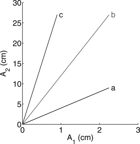
The performance of the estimators was measured in terms of the MSE, the bias, and the variance of the output with noisy data. In general, the results will depend on the object attenuation, so they were measured along a set of lines through the A-plane shown in Fig. 6. The points on each line correspond to different thicknesses of a particular material. The results were then plotted as a function of the distance along this line from the origin, which is proportional to the material thickness.

Figure 6.

Lines in A-plane for evaluation of errors. The errors are evaluated for objects with attenuation A-vectors on this line and plotted as a function of the distances along the lines from the origin.

Errors with low-noise data vs number of calibrator steps

Estimates with polynomial, rational polynomial, and A-table estimators were computed for 25 points along line (b) in Fig. 6 with deterministic values, i.e., using the mean values of the data. The errors were the differences between the estimates of the A-vector components and the actual values. This was taken to be the bias although the nonlinear transformation of the mean is not necessarily equal to the mean of the transformation of the noise. In our case, the near linearity of the transformation, shown in Fig. 2, implies that the bias will be close to the transformation of the mean. The average of the absolute value of the errors is displayed as a function of the number of steps in the calibrator step wedges.

Estimator variance and MSE

The estimator variance and MSE were simulated as a function of object thickness for data from a PHA detector with two to five bins. They were computed for 200 Monte Carlo trials at each of the points along the lines in the A-plane in Fig. 6. As discussed above, the variance is the expected value of the square of the difference of the output and its mean value. It was estimated using the sample variance of the Monte Carlo trials

$$\mathrm{var}(\stackrel{\wedge }{\mathbf{A}})=\frac{1}{m-1}\sum _{i=1}^m{({\stackrel{\wedge }{\mathbf{A}}}_i-\stackrel{-}{\stackrel{\wedge }{\mathbf{A}}})}^2,$$

where $\stackrel{-}{\stackrel{\wedge }{\mathbf{A}}}$ is the mean of the estimator output and m is the number of Monte Carlo trials. The MSE was computed using the known value of A at each point

$$\mathrm{MSE}(\stackrel{\wedge }{\mathbf{A}})=\frac{1}{m}\sum _{i=1}^m({\stackrel{\wedge }{\mathbf{A}}}_i-\mathbf{A}){}^2.$$

The covariance used in the linear MLE of the A-table method was estimated from 5 × 10⁴ trials. The incident 120 kV x-ray tube spectrum at each pixel was assumed to have a total of 10⁶ photons. The bin energy regions were selected to give an equal number of transmitted photons in each bin at the attenuation of an object with 2.5 cm of aluminum and 15 cm of plastic. A 40 step calibration phantom was used.

The CRLB was computed at each point along the line using the formula described in Sec. 2E with the transmitted spectra for the object attenuation at each point.

The standard error of the variance for each point along the line was computed using the bootstrap method¹⁸ with 100 iterations.

CRLB vs number of bins

The simulator also allows us to compute the CRLB as a function of the number of PHA bins. The object A-vector was fixed at 2.5 cm of aluminum and 15 cm of acrylic plastic. The incident spectrum was a TASMIP 120 kV x-ray tube spectrum with 10⁶ photons. The bin widths were adjusted to give equal counts in all bins.

RESULTS

Errors vs number of calibrator steps

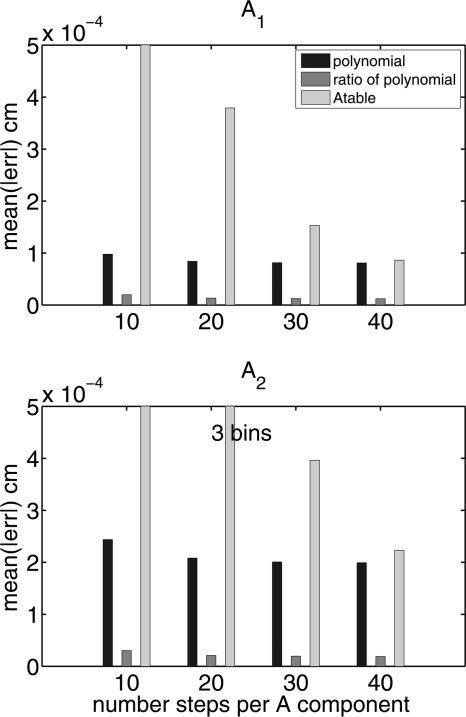
The average errors with deterministic data are shown in Fig. 7 as a function of the number of steps of the calibration phantom shown in Fig. 3. These are the steps for each component; so, the number of regions in the phantom is the square of the number of steps. The polynomial and ratio of polynomial estimators are given by Eqs. 16, 17.

Figure 7.

The mean of the absolute value of the errors vs the number of steps of the calibrator step wedges. At each step number, there are three error bars corresponding to each type of estimator. The errors for the two A-vector components are plotted separately.

Variance and MSE vs object thickness

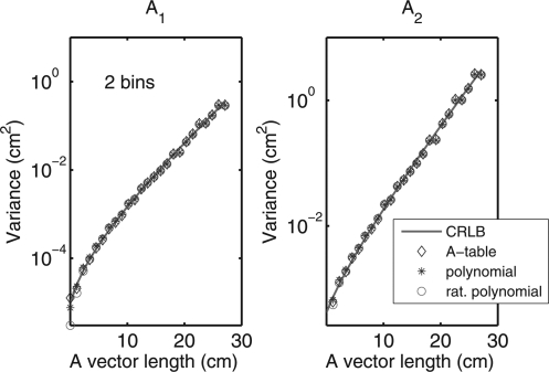
The variance of the estimates for PHA data with two bins is plotted in Fig. 8. The CRLB is plotted as a solid line, and the Monte Carlo results are plotted as individual symbols. The data correspond to points in the A-plane along line (b) of Fig. 6. Notice that with two bins all the estimators have approximately the same variance and all achieve the CRLB. In this case and the other cases considered below, the MSE was essentially equal to the variance so that the bias was negligible.

Figure 8.

Variance of estimator output for PHA data with two bins for data on line (b) in Fig. 6. The results are shown for the A-table, polynomial, and rational polynomial estimators. The A-vector length is the distance from the origin on the line. The data are plotted in semilogarithmic scales because of their wide variation. The CRLB is plotted as the solid curve. In this case, the variances of all estimators are essentially the same and equal to the CRLB.

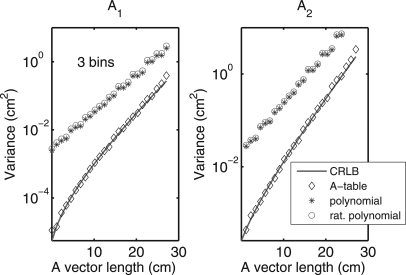
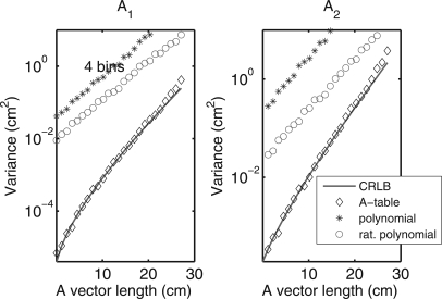
The variance with three bins is shown in Fig. 9. The A-table estimator achieves the CRLB but with three or more bins, the polynomial and rational polynomial estimators’ variance was much larger, over a factor of 100 in some cases. The variance of the alternate estimators was equal for three bins but was different for four bins as shown in Fig. 10.

Figure 9.

Variance for PHA data with three bins on line (b) in Fig. 6. With three bins, the polynomial and rational polynomial results are essentially equal but are much larger than the A-table results, which are shown as black diamonds. The A-table results are essentially equal to the CRLB.

Figure 10.

Variance for PHA data with four bins on line (b) in Fig. 6. With four bins, the polynomial and rational polynomial results are different but are both much larger than the A-table results, which are shown as black diamonds. The A-table results are essentially equal to the CRLB.

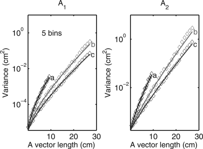
The variance of the A-table estimator with five bins was evaluated for all three lines in the A-plane in Fig. 6. The results are in Fig. 11.

Figure 11.

Variance for A-table estimator with five bin PHA data. The labels on the data correspond to the lines in Fig. 6. The CRLB is plotted as a solid line while the variances are plotted as diamonds.

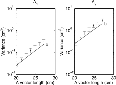
The data for line (b) in Fig. 11 seem to show a deviation from the CRLB at the largest object thicknesses. The data in this region are replotted in Fig. 12 with error bars corresponding to ±2 standard deviations of the estimates computed using the bootstrap method described in Sec. 3A

Figure 12.

Replot of data for the region at the end of line (b) of Fig. 11 with error bars corresponding to ±2 standard deviations. In this region, the variance deviates from the CRLB although the differences are only approximately twice the standard deviation of the variance estimates from the Monte Carlo simulation.

CRLB vs number of bins

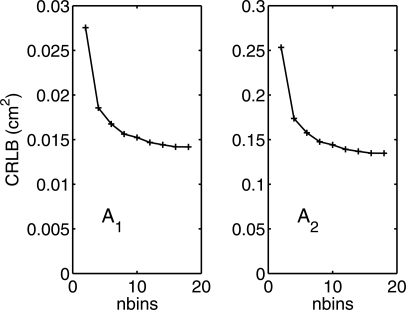
The CRLB as a function of the number of PHA bins is shown in Fig. 13. Recall that the bin widths were adjusted to give equal counts in all bins so that the widths are not equal.

Figure 13.

CRLB as a function of the number of PHA bins for an object consisting of 2.5 cm of aluminum and 15 cm of acrylic plastic. The two panels show the variances of the A-vector components. The number of bins ranges from 2 to 18.

DISCUSSION

Alvarez and Macovski² showed that the MLE for two spectra simply solves the deterministic equations with the measured data and that the MLE achieves the CRLB. Therefore, the output noise variance for all two spectra estimators that solve the equations accurately is essentially the same and this is reflected in the results in Fig. 8. With three and four bin data, Figs. 910 show that the polynomial and rational polynomial estimators have variance substantially larger than the A-table method, which essentially achieves the CRLB, and the variances are larger than with two bin data.

The multibin data could be summed together to produce two bin data, which would have lower variance than the results in Figs. 910, but this would not provide the lower output noise with increased number of bins shown in Fig. 13. It may be possible to precompute the maximum likelihood estimates throughout the L measurement space with an iterative MLE and then compute a polynomial or other function fit to the data. However, previous iterative MLE implementations, such as Schlomka et al.,¹¹ required high resolution measurements of the spectra and detector response that may not be practical for clinical applications. In addition, the “curse of dimensionality” would require complex fit functions with a large number of undetermined coefficients for higher dimensional data. Other ways of computing a polynomial or rational polynomial fit are, of course, possible but they cannot have a smaller variance than the CRLB if they are unbiased.

Figures 1112 show the A-table estimator may have a small systematic deviation from the CRLB at the largest object thicknesses. At large thicknesses, the covariance differs from the average value assumed in the initial linear estimator; so, this leads to errors that are not corrected sufficiently by the look up table. Nevertheless, Fig. 11 shows that for almost all the A-plane region of interest, the A-table estimator achieves the CRLB.

Figure 7 shows the bias errors with deterministic data as a function of the number of steps in the calibration phantom. The A-table estimator errors are substantially larger than the other estimators for small number of steps but become comparable to the polynomial estimator errors for 40 steps. The errors with the rational polynomial estimator are the smallest. For the range of photon counts studied, which were chosen to be representative of clinical systems, the MSE is dominated by the variance for all estimators indicating that the bias does not substantially affect the overall performance of the estimators.

A 40 step calibration phantom requires 1600 data points; so, the measurements should be extracted automatically under software control. The dimensions of the calibration phantom can be built into the software and the data can be acquired using a standard procedure and with the phantom placed at a predetermined position. The phantom size and data acquisition time can be adjusted to give calibration data with low-noise. An additional scan with technique similar to that used during patient imaging may be used to provide data to estimate the noise covariance. This may require different calibrations for each scan technique but it may be possible to parametrize the results to adjust them for specific cases. Beam divergence implies that the lengths through each region of the phantom differ slightly. This may be minimized by using nonplanar surfaces in the calibration phantom steps and by computing an effective thickness for the geometry of each step.

A possible alternative to the look up table is to approximate the correction functions in the A-plane with two-dimensional polynomials, sinusoids, or other smooth functions. It may be difficult to approximate the portion of the correction functions near the origin because of the high gradient there. In addition, the fact that the sampled functions are not available on a rectangular grid may cause difficulties in computing the approximation.

Figure 13 shows that the CRLB decreases as the number of PHA bins increases and asymptotically approaches a lower limit. Although the CRLB values for low number of bins depend on the choice of the bin thresholds, the choice has less effect as the number of bins increases so that there is a well defined lower limit. The CRLB is closely related to the optimal signal to noise ratio (SNR) from statistical detection theory described in my previous paper.¹⁵ The SNR depends on the full CRLB matrix but the asymptotic approach of the variances to a lower limit is consistent with the result in that paper, which shows that the SNR approaches the Tapiovaara–Wagner¹⁹ optimal SNR as the number of bins increases.

Factors such as pulse pileup, low energy spectral distortion due to charge sharing and K radiation escape, and scatter within the patient were not considered here but are currently being studied. The success of Schlomka et al.¹¹ in producing experimental images with an iterative MLE indicates that these problems may be able to be addressed. Further, the state of the art of photon counting detectors for medical imaging is progressing rapidly. For example, in 2007, Iwanczyk et al.²⁰ reported making clinical CT images with photon counting detectors albeit at reduced dose. Using the A-table estimator with improved counting detectors and count rate dependent correction of errors as a preprocessing step could produce low-noise, energy-selective images.

The use of multibin PHA data to image high atomic number contrast material is of substantial interest. In this case, the two function basis is not accurate because of the K-edge of the contrast material attenuation coefficient within the energy region of interest. This can be accommodated by extending the basis set to three functions by adding the attenuation coefficient of the contrast material. The A-table estimator may be generalizable to this case. The linear MLE can be readily extended to three dimensions and 3D look up tables can be implemented. The calibration phantom would require additional wedges of the contrast material or perhaps a material simulating the contrast agent in the surrounding body tissue. Automated procedures could be used to acquire the data.

CONCLUSION

The operation of a noniterative estimator for the energy dependent information from photon counting detectors with multibin pulse height analysis data is described and its performance evaluated using a Monte Carlo simulation. The estimator is implemented as a matrix multiplication followed by a two-dimensional look up table so that its computation time is fast and predictable. It achieves the Cramèr-Rao lower bound with all the detector types studied for all object thicknesses except for a small deviation at large object thickness. Therefore, we are guaranteed that no other unbiased estimator can have smaller variance in the region where it achieves this bound. Its bias is small enough that the mean square error is dominated by the variance in all cases. The parameters required to implement the estimator can be derived from transmission data with a calibration phantom and do not require measurements of the source spectrum or the detector energy response functions.

Alternate fast noniterative estimators based on least squares polynomial and rational polynomial approximations of the inverse transformation are also studied. While these estimators provide low bias, their output noise variance, as implemented here by fitting to noise-free calibration data without optimization for noise performance, is much larger than the A-table estimator variance and the Cramèr-Rao lower bound.

References

- Aslund M., Fredenberg E., Telman M., and Danielsson M., “Detectors for the future of x-ray imaging,” Radiat. Prot. Dosim. 139, 327–333 (2010). 10.1093/rpd/ncq074 [DOI] [PubMed] [Google Scholar]
- Alvarez R. E. and Macovski A., “Energy-selective reconstructions in x-ray computerized tomography,” Phys. Med. Biol. 21, 733–744 (1976). 10.1088/0031-9155/21/5/002 [DOI] [PubMed] [Google Scholar]
- Cardinal H. N. and Fenster A., “An accurate method for direct dual-energy calibration and de composition,” Med. Phys. 17, 327–341 (1990). 10.1118/1.596512 [DOI] [PubMed] [Google Scholar]
- Chuang K.-S. and Huang H. K., “A fast dual-energy computational method using isotransmission lines and table lookup,” Med. Phys. 14, 186–192 (1987). 10.1118/1.596110 [DOI] [PubMed] [Google Scholar]
- Hassler U., Garnero L., and Rizo P., “X-ray dual-energy calibration based on estimated spectral properties of the experimental system,” IEEE Trans. Nucl. Sci. 45, 1699–1712 (1998). 10.1109/23.685292 [DOI] [Google Scholar]
- Zhang G., Cheng J., Zhang L., Chen Z., and Xing Y., “A practical reconstruction method for dual energy computed tomography,” J. X-Ray Sci. Technol. 16, 67–88 (2008). [Google Scholar]
- Stenner P., Berkus T., and Kachelriess M., “Empirical dual energy calibration (EDEC) for cone-beam computed tomography,” Med. Phys. 34, 3630–3641 (2007). 10.1118/1.2769104 [DOI] [PubMed] [Google Scholar]
- Kay S. M., Fundamentals of Statistical Signal Processing, Vol. I: Estimation Theory (Prentice-Hall PTR, Upper Saddle River, NJ, 1993). [Google Scholar]
- Van Trees H. L., Detection, Estimation, and Modulation Theory Part I: Detection, Estimation, and Linear Modulation Theory, 1st ed. (John Wiley & Sons, New York, 2001). [Google Scholar]
- Roessl E. and Proksa R., “K-edge imaging in x-ray computed tomography using multi-bin photon counting detectors,” Phys. Med. Biol. 52, 4679–4696 (2007). 10.1088/0031-9155/52/15/020 [DOI] [PubMed] [Google Scholar]
- Schlomka J. P., Roessl E., Dorscheid R., Dill S., Martens G., Istel T., Bäumer C., Herrmann C., Steadman R., Zeitler G., Livne A., and Proksa R., “Experimental feasibility of multi-energy photon-counting K-edge imaging in pre-clinical computed tomography,” Phys. Med. Biol. 53, 4031–4047 (2008). 10.1088/0031-9155/53/15/002 [DOI] [PubMed] [Google Scholar]
- Wang J., Lu H., Liang Z., Eremina D., Zhang G., Wang S., Chen J., and Manzione J., “An experimental study on the noise properties of x-ray CT sinogram data in Radon space,” Phys. Med. Biol. 53, 3327–3341 (2008). 10.1088/0031-9155/53/12/018 [DOI] [PMC free article] [PubMed] [Google Scholar]
- Alvarez R. E. and Seppi E. J., “A comparison of noise and dose in conventional and energy selective computed tomography,” IEEE Trans. Nucl. Sci. NS-26, 2853–2856 (1979). 10.1109/TNS.1979.4330549 [DOI] [Google Scholar]
- D’errico J., “Surface Fitting using gridfit.” [Online]. Available: MATLAB Central File Exchange, http://www.mathworks.com/matlabcentral/fileexchange/8998. [Google Scholar]
- Alvarez R. E., “Near optimal energy selective x-ray imaging system performance with simple detectors,” Med. Phys. 37, 822–841 (2010). 10.1118/1.3284538 [DOI] [PMC free article] [PubMed] [Google Scholar]
- Boone J. M. and Seibert J. A., “An accurate method for computer-generating tungsten anode x-ray spectra from 30 to 140 kV,” Med. Phys. 24, 1661–1670 (1997). 10.1118/1.597953 [DOI] [PubMed] [Google Scholar]
- Devroye L., Non-Uniform Random Variate Generation (Springer-Verlag, Berlin, 1986). [Google Scholar]
- Efron B. and Tibshirani R., An Introduction to the Bootstrap (CRC, Boca Raton, FL, 1993). [Google Scholar]
- Tapiovaara M. J. and Wagner R., “SNR and DQE analysis of broad spectrum X-ray imaging,” Phys. Med. Biol. 30, 519–529 (1985). 10.1088/0031-9155/30/6/002 [DOI] [Google Scholar]
- Iwanczyk J., Nygard E., Meirav O., Arenson J., Barber W., Hartsough N., Malakhov N., and Wessel J., “Photon counting energy dispersive detector arrays for x-ray imaging,” IEEE Nuclear Science Symposium Conference Record, Vol. 4, pp. 2741–2748 (2007). [DOI] [PMC free article] [PubMed] [Google Scholar]