Performance comparison of machine learning algorithms and number of independent components used in fMRI decoding of belief vs. disbelief

Abstract

Machine learning (ML) has become a popular tool for mining functional neuroimaging data, and there are now hopes of performing such analyses efficiently in real-time. Towards this goal, we compared accuracy of six different ML algorithms applied to neuroimaging data of persons engaged in a bivariate task, asserting their belief or disbelief of a variety of propositional statements. We performed unsupervised dimension reduction and automated feature extraction using independent component (IC) analysis and extracted IC time courses. Optimization of classification hyperparameters across each classifier occurred prior to assessment. Maximum accuracy was achieved at 92% for Random Forest, followed by 91% for AdaBoost, 89% for Naïve Bayes, 87% for a J48 decision tree, 86% for K*, and 84% for support vector machine. For real-time decoding applications, finding a parsimonious subset of diagnostic ICs might be useful. We used a forward search technique to sequentially add ranked ICs to the feature subspace. For the current data set, we determined that approximately six ICs represented a meaningful basis set for classification. We then projected these six IC spatial maps forward onto a later scanning session within subject. We then applied the optimized ML algorithms to these new data instances, and found that classification accuracy results were reproducible. Additionally, we compared our classification method to our previously published general linear model results on this same data set. The highest ranked IC spatial maps show similarity to brain regions associated with contrasts for belief > disbelief, and disbelief < belief.

Introduction

In the early 1950s, Shannon developed an iterated penny-matching device designed to perform simple “brain reading” tasks (Shannon, 1953). Although this device performed only slightly better than chance, it created a fascination with brain reading technology (Budiansky et al., 1994). Recent advancements in neuroimaging have provided a quantitative method for visualizing brain activity that corresponds to mental processes (Cox and Savoy, 2003), and certain brain reading feats have been accomplished by applying pattern classification techniques to functional magnetic resonance imaging (fMRI) data (Norman et al., 2006).

The application of machine learning (ML) to fMRI analysis has become increasingly popular, following its initial application to Haxby's visual object recognition data (Hanson et al., 2004). Neural networks (Hanson et al., 2004), Naïve Bayes (Pereira et al., 2009), and support vector machine classifiers (LaConte et al., 2005) each have yielded varying levels of predictive capability. However, fMRI data sets are extremely large, and one of the key challenges in fMRI classification has been to mine these vast data effectively.

Although certain studies have used the entire fMRI data set for predictive purposes (LaConte et al., 2007), most investigators perform a preliminary dimension reduction step to reduce the number of inputs used for classification. Reducing dimensionality has a number of benefits; specifically, computational burden is reduced and classification efficiency is often improved, and problems with over-fitting that may lead to poor generalization are reduced (Yamashita et al., 2008).

Determining an optimal method for dimension reduction is an active area of research. Physiologically driven approaches for data reduction have been employed to incorporate spatial dependencies. For example, selecting regions of interest (ROIs) in the brain, diminishes input size substantially (Cox and Savoy, 2003). However, these techniques typically require user-input and a priori knowledge about brain morphology associated with a given task (Mourão-Miranda et al., 2006). Searchlight analysis (Kriegeskorte et al., 2006) has yielded powerful results. Multivoxel pattern analysis (Norman et al., 2006) and sparse logistic regression (Yamashita et al., 2008) provide useful methods for determining voxel subsets with high signal-to-noise ratio. However many voxels, especially those in adjacent spatial locations, may provide approximately the same information, and subsets of voxels selected may differ fold to fold. Using a method like independent component analysis (ICA) allows basis images to cover the entire brain, and may prove to be a more reproducible method for parsimonious dimension reduction.

Here, we utilized independent component analysis (ICA) as an unsupervised method for both dimension reduction and feature extraction. ICA is a powerful blind source separation technique that has found numerous applications in the field of functional neuroimaging to include: data exploration (Beckmann et al., 2006), noise component elimination (Tohka et al., 2008), and more recently by our group (A. Anderson et al., 2009) as a dimension reduction technique in fMRI ML classification. We hypothesize that ICs themselves may represent a reasonable basis to describe certain brain states. To the extent that this is true, output from certain classifiers could be interpreted as a weighting of these primitive bases to describe higher-level cognitive states.

Lack of parameter optimization at key steps along an fMRI data processing pipeline can substantially affect analysis outcome (Strother et al., 2004). Here, we have paid particular attention in parameter optimization at multiple steps in the decoding process. First, we compare classification accuracy using six different ML classifiers, across a range of complexity. Where applicable, hyperparameters within ML algorithms were also optimized simultaneously with optimizing the number of IC features. Optimal feature subset selection has been useful a number of fields (Dash and Liu, 1997) where machine learning has been applied including: brain computer interfaces (Garrett et al., 2003), voice recognition (Pandit and Kittler, 1998), and in classifying gene microarray expression data (Bo and Jonassen, 2002). Nonetheless, there have been relatively few efforts to perform this analysis on fMRI data. Optimal feature selection can clearly improve computational efficiency, which may be a consideration when applying tools in near real-time, especially in a neurofeedback protocol. However, there are multiple reasons why this optimization step is useful when computation time is not a consideration. Improved classification accuracy (Kohavi, 1997), reduced data storage requirements (Aha, 1992), and diminished probability of overfitting (Hastie et al. 2001) are three motivating factors. Generalization capability also increases with the ratio of training patterns to features (Theodoridis and Koutroumbas 2009).

For the experiments performed here we utilized a previously published data set (Harris et al., 2008). Some of the present results have been shown in abstract form (Douglas et al., 2009, 2010).

Methods

Overview

Our methodology, in brief, is as follows:

1. Data Preprocessing

2. Dimension Reduction & Feature Extraction Using ICA

3. Machine Learning Algorithms

4. Training, Testing, and Iterative Optimization

5. Comparison across Classifiers and Feature Subsets.

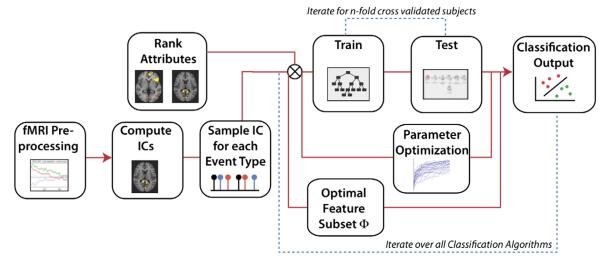
This methodology was applied within subject. A variety of decision criterion were aplied to determine the optimal number of features. A block diagram illustrating this methodology is shown, Fig. 1.

Fig. 1.

Methodology flow diagram. Following preprocessing steps that included motion correction and brain extraction, independent component analysis (ICA) was performed and time courses associated with each spatial IC were sampled for “belief” and “disbelief” conditions. IC component features were ranked and then sent as inputs into machine learning for training and testing of the classifier, which proceeds over an n-fold cross-validated sample. Classifier parameters are adjusted and optimized.

Study data

Prior to the experiment we obtained IRB approval from UCLA and written informed consent from fourteen healthy adult subjects (18–45 years old; 7 women) with no medical history of psychiatric disorder, as assessed by a medical history survey. Participants underwent three 7-minute functional MRI scans (Siemens Allegra 3T). Each scanning session consisted of ~100 trials, yielding a total of ~300 trials per subject. While in the scanner, subjects were presented with short statements through video goggle displays. The presentation of stimuli was self-paced, with an inter-stimulus interval of 500 ms. Subjects were asked to evaluate the truth content from seven different statement categories: mathematical, ethical, factual, geographic, autobiographical, religious, and semantic. After reading each statement, subjects were asked to press a button indicating that they believed, disbelieved or were uncertain about the veracity of each statement. These data were collected as part of a published study (Harris et al., 2008) but are re-analyzed here.

Data preprocessing

FMRI preprocessing included conventional motion correction (Jenkinson et al., 2002) and brain extraction (Smith et al., 2002), and was carried out using FSL (www.fmrib.ox.ac.uk/fsl).

Dimension reduction and feature extraction using ICA

We performed a global ICA computation on each subject's data set. ICA is a powerful tool for finding hidden factors that underlie multivariate data. Known input data is decomposed into a linear combination of statistically independent latent variables, or components, in an unknown mixing system, A. When applied to fMRI, the data are four-dimensional: q different voxel intensities are measured at p different time points. Spatial data is first unwrapped and a two dimensional q by p matrix, X, is formed, where columns and rows represent spatial and temporal data, respectively. Classic ICA proceeds by the following decomposition:

$$\mathbf{X}=\mathbf{AS}.$$ (1)

The matrix S is optimized to obtain statistically independent spatial maps that correspond to various regions of the brain with corresponding temporal aspects. This representation avoids making specific assumptions, as occurs with regression or the general linear model. However, it does not treat the possible introduction of noise. Probabilistic ICA introduces Gaussian noise to the model with the underlying assumption that the p column vector is generated by q statistically independent non-Gaussian sources in a mixing process that is corrupted by the addition of noise, φ:

$${\mathit{x}}_{\mathit{i}}=\mathbf{As}+\mathrm{\mu }+\mathrm{\phi },$$ (2)

where x_i is a p-dimension vector of measurements at voxel location i. and μ is the mean of x_i observations. In order to solve the equation a linear transformation matrix W is required such that:

$$\mathbf{s}=\mathbf{Wx},$$ (3)

which provides a close approximation to the source of the signals s. Probabilistic ICA was performed here, using the methodology described above, which forms the basis for the computational program FSL MELODIC, (Beckmann et al., 2006).

IC timecourse values were then extracted and sampled at time points corresponding to belief and disbelief events, and assigned the appropriate class label. More specifically, we modeled belief and disbelief events as delta functions, δ(t), occurring at the mean time point between stimulus onset and subject keypad response. These delta functions were then convolved with the conventional double gamma hemodynamic response function, as implemented in the SPM software package, to calculated the predicted blood oxygenation level dependent (BOLD) response. IC timecourses were sampled at time points corresponding to the maximum predicted BOLD response value. Due to the rapid, self-paced experimental paradigm used in the Harris et al., 2008 study, multiple belief and disbelief events sometimes occurred within a single TR. To avoid overlap in these cases, we included only those data instances whose class label was identical for two or more consecutive trials. Effectively, this sampling process reduced the number of data exemplars included by approximately one third. Extracted IC timecourse features were subsequently used as inputs in our classification analysis.

Classification techniques

We evaluated six machine learning algorithms over a range of complexity, each of which was implemented and automated using Perl, WEKA (University of Waikato, New Zealand), and MATLAB (v.7.6, Mathworks, Inc.) software. We describe each of these briefly here.

K-Star

K* is a simple, instance based classifier, similar to K-Nearest Neighbor (K-NN). New data instances, x, are assigned to the class that occurs most frequently amongst the k-nearest data points, y_j, where j = 1,2…k (Hart, 1968). Entropic distance is then used to retrieve the most similar instances from the data set. Using entropic distance as a metric has a number of benefits including handling of real valued attributes and missing values (Cleary and Trigg, 1995). The K* function can be calculated as:

$$K^{\ast }(y_i,x)=-\mathit{ln}{P}^{\ast }(y_i,x)$$ (4)

where P* is the probability of all transformational paths from instance x to y. It can be useful to interpret this as the probability that x will arrive at y via a random walk in IC feature space. We performed optimization over the percent blending ratio parameter, which is analogous to K-NN ‘sphere of influence’, prior to comparison with other ML methods.

Naïve Bayes

We applied Naïve Bayes' classification to our belief, disbelief discrimination task as follows. Posterior probabilities P(C_i|x), or conditional probability of observing class, C_i, given data instance, x were computed as:

$$P(C_i\mid x)=\frac{P\left(C_i\right)p(x\mid C_i)}{p\left(x\right)},$$ (5)

where, P(C_i) is the prior probability of C_i occurring, class likelihood P(x|C_i) is the conditional probability that an event in class C is associated with observation x, and P(x) is the marginal probability that an event x is observed. Maximum a posteriori thresholding P(C_i|x) was then applied:

$$\{\begin{array}{cc}{C}_i=B\hfill & \mathit{if}P(C_i\mid x)>\mathrm{\xi }\hfill \\ C_i=\stackrel{-}{B}\hfill & \mathit{else}\hfill \end{array}\phantom{\}},$$ (6)

As individual features are assumed to be statistically independent in the IC computation, we extend this to assume independent conditional probabilities, as is the case in the Naïve Bayes classifier, computed for each (j = 1, …N) IC time course:

$$P(x\mid C_i)=\prod _{j=1}^{N}p\left(x_j\mid C_j\right).$$ (7)

Support vector classifier

Support vector machine (SVM) (Vapnik, 2000; Burges, 1998) were assessed for their belief/disbelief discrimination capability, since SVM algorithms are computationally stable, generalize well, and have been applied successfully to microarray (Golub et al., 1999) and fMRI (LaConte et al., 2005) data. The SVM classifiers find the maximum-margin hyperplane using only those data instances that are closest to the separation boundary or “support vectors” to determine soft margin for classification (Corinna and Vapnik, 1995). Nonlinearly separable data may be projected into a space of higher dimensionality with the use of a kernel function, making hyperplane separation in this new space occur more readily. Here we optimized across multiple kernel functions prior to classification assessment via cross validation.

Decision tree

We applied the J48 decision tree based on the C4.5 algorithm (Quinlan, 1993) here, which proceeds by partitioning data into local sets using a series of recursive splits. Tree generation then begins with a root node, which utilizes all training data to search for the best splitting of the data. Partitioning continues until a terminal leaf node, where data instances are assigned a class label (Alpaydin, 2004). At each decision node, a threshold is applied sending incoming data instances into the appropriate branch of the tree. The partitioning threshold is calculated by selecting values that result in the largest decrease in impurity. This was calculated by taking the difference of the impurity, I, at node m:

$$I_m=\underset{j=1}{\overset{k}{\Sigma }}{p}_{\mathit{mj}}^i{\mathit{lnp}}_{\mathit{mj}}^i$$ (8)

from the total impurity in the system:

$$I_{\mathit{total}}=\underset{j=1}{\overset{n}{\Sigma }}\frac{N_{\mathit{mj}}}{N_m}\underset{j=1}{\overset{k}{\Sigma }}{p}_{\mathit{mj}}^i{\mathit{lnp}}_{\mathit{mj}}^i$$ (9)

where

$$p_{\mathit{mj}}^i=\frac{N_{\mathit{mj}}^i}{N_m}$$ (10)

Here, N_m is the number of data instances at node m, j is the branch, and i is the class label. A split is considered pure if, after the split, all instances at the downstream nodes belong to a single class. Additional branches in the tree are added in a similar fashion until a specified purity threshold is reached, and instances at each terminal node are assigned a class label. Pruning options were varied here, for optimization.

AdaBoost classification

AdaBoost is an adaptive boosting algorithm, whereby linear combinations of weak classification features are constructed into a robust classifier. Initially the weights on each feature are uniform. The most discriminatory feature is then reweighted to count more substantially in the prediction outcome. The feature that most accurately discriminates data instances that were misclassified by the first feature is selected next (Viola and Jones, 2001). Because of this, a feature that is weak in a few examples would be compensated by a feature that necessarily performed strongly on those same samples. The first classifier a boosting algorithm selects is always the minimum-error weak classifier. Boosting is a “greedy” algorithm that ultimately combines weak classifiers into a strong classifier, and always accepts the additional classifier that most strongly reduces the classification error at that particular iteration.

Random Forest

Random Forest algorithms employ a technique known as bagging, whereby data instances are resampled multiple times to produce multiple training subsets from the training data. Decision trees are then created from each training subset, until ensembles of trees have been created (Breiman, 1996). Each tree then casts a unit vote for the outcome of an incoming data instance class label. This is different from Adaboost where each weak classifier casts a weighted vote. Here we used the method developed by (Breiman, 2001), where individual class labels, i, are assigned based on the mode or most popular class label is assigned to the input.

Training, testing and iterative optimization of classifiers

Training

Data instances from each subject's data were partitioned randomly into ten equal sets. Nine of these sets were used for training purposes, called the training data, which we denote here as, d. The tenth subset of data was used for testing and validation purposes. This data partitioning was done in order to avoid ‘double dipping’ (Kriegeskorte et al., 2009). Following feature extraction, data parsed into the training set was used for IC ranking. A t-test was applied to each IC's data for belief and disbelief conditions, and ICs were then sorted based on corresponding t-statistic. Ranking based on t-statistic is a computationally efficient method that has proven useful in a number of applications including microarray gene expression data (Liu et al., 2002).

Testing

The tenth data subset was then used for testing and validation purposes. We then cycled through all blocks, such that each of the ten data subsets was given a chance to be the test set, in a process known as 10-fold cross validation, as also described in the decoding study by Norman et al. (2006). Classification accuracy was assessed as the percentage of data instances that were labeled correctly after repeating this process ten times (Pereira et al., 2009).

Hyperparameter optimization via nested cross validation

ML Algorithms optimize certain internal parameters based training data and minimization of cost functions. In SVM classifiers, for example, the maximum-margin hyperplane for shattering data is optimized based on training data. Certain algorithms also have hyperparameters, which must also be adjusted to data, but are not optimized in the training process. In order to optimize these hyperparameters, we performed a nested cross validation, as has been done for brain–computer interface ML applications (Muller et al., 2004). In this process, an inner cross validation is used to optimize hyperparameter values, which are then applied to the outer set. In this sense, data exemplars that were used for classification accuracy assessment were kept in a ‘vault’ until the final evaluation of the outer cross validation. Ten-fold cross validation was used for both outer and inner sets. Specifically, we optimized over the percent blending ratio for K*, a variety of kernel functions in SVM, the pruning ratio for decision trees, the threshold for weight pruning in Adaboost, and the number of iterations used in Random Forest.

Optimal feature subset selection

Forward search selection

Our objective is to select the set of components that will result in the highest percent of correct classification using a minimal number of features. Here, we utilized a forward search selection approach, whereby we start with no components and add on additional ICs in order of increasing rank based on t-statistic. We truncated this analysis at d = 25 components, at which point misclassification error on the test set had become asymptotic. Stop criterion for this process are described below.

Stop criterion for forward selection

Rise threshold

Here, we utilize a control systems measure known as ‘rise time’ as means for truncating the forward selection process. Additional ICs attributes are successively added until classification error is less than or equal to a threshold, ς, of the maximum correct classification achievable when d = 25 IC components are included, which we use as our baseline, β. Specifically,

$${\mathit{IC}}_{\mathrm{rt}}=\text{set of}{\mathrm{IC}}_{\mathrm{i}}\text{such that}E\left({\mathit{IC}}_{\mathit{rt}}\right)\le {\mathrm{\varsigma }}^{\ast }\mathit{max}\left(1-E\left({\mathit{IC}}_{\mathrm{\beta }}\right)\right).$$ (11)

Here the term, ς, represents what we are calling the rise threshold, which can be modified to accommodate different tolerances on misclassification rates.

Classification output curve fitting

Modeling classification output may be useful in assessing stop criteria for adding additional ICs to the classification vector. Mean classification accuracy as a function of the number of ICs (N_ICs) was averaged across all subjects. Using a Marquardt–Levenberg algorithm (Marquardt, 1963), we fitted these output curves to a first order exponential model of the form:

$$E\left({\mathit{IC}}_d\right)=E\left({\mathit{IC}}_{\mathrm{\varphi }}\right)+\left(E\left({\mathit{IC}}_{\mathrm{\beta }}\right)-E\left({\mathit{IC}}_{\mathrm{\varphi }}\right)\right)\left[1-e^{-d∕\lambda }\right]$$ (12)

where, d is the number of ICs, E(IC_ϕ) is the accuracy with a single IC, E(IC_β) − E(IC_ϕ) is the asymptotic accuracy, and λ describes the rate of asymptotic classification performance.

IC projection to other scans within subject

For certain applications, it may be useful to avoid the computational bottleneck incurred by pICA calculation. We, therefore, selected informative IC features for projection onto future scanning sessions within subject. Binary IC spatial maps that resulted from the FSL MELODIC computation were projected onto incoming functional data. Mean time series from each of these projections were extracted and used as features for classification.

Results

Hyperparameter optimization

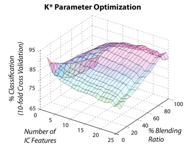
Each classification algorithm was optimized over key hyperparameters jointly with the number of IC attributes. Optimization for K* was varied over percent blending ratio, which corresponds to the sphere of influence in K-NN. We found that a single order polynomial kernel was optimal for SVM, an 86% blending ratio was optimal for K* (Fig. 2), and a 10% pruning ratio for our J48 decision tree.

Fig. 2.

Algorithm parameter optimization for K* classification. Output averaged across all subjects and trial runs for varying numbers of ICs and % blending ratios.

Performance comparison across classifiers

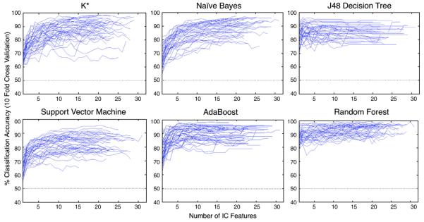
Classification results using optimal parameter values across all six classifiers are shown in Figs. 3 (a–f). Each curve represents classification output for a single subject run. Here, the highest ranked component was added first, following with the second highest ranked component, until all components had been included in the set considered by the classifier. We used a 10-fold cross validation approach for training and testing each method. We partitioned the data randomly into 10 sets, where 9 sets were used to train the classifier and 1 set, representing 10% of the data was used to test. We rotated the training and test sets until all of the data sets had been used for testing. It should be noted that the total number of ICs varied across data sets.

Fig. 3.

(a–f). Classification results using forward selection method for each subject for (a) K* (b) Naïve Bayes (c) J48 decision tree (d) support vector machine (e) Random Forest, and (f) AdaBoost, with chance for bivariate classification (50%) indicated with a dashed line.

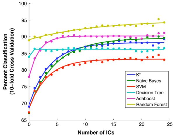
In order to determine how many components to include for the group as a whole, we computed the mean classification accuracy across all subjects as a function of the number of ICs included in the classification vector (Fig. 4). These means generally increased monotonically as more components were considered, until an asymptotic performance was reached. This was approximately the case for three of the classifiers. In the case of the K*, the results degraded beyond considering two components. The percent correct classification rose rapidly for AdaBoost and then leveled off. Naïve Bayes produced comparable results to AdaBoost, when a large number of components were considered.

Fig. 4.

Classification accuracy averaged across all subjects, shown for each of the six classifiers as a function of the number of ICs, with fits to 3-parameter first order exponential model (lines).

Classification across number of ICs

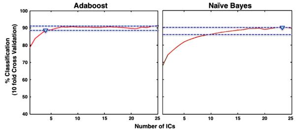
We applied three measures to truncate our forward feature selection process. A rise threshold of 95% was applied to each classifier, using the classification accuracy achieved using 25 ICs as a baseline. In all but one of the classifiers, the number of components needed to achieve specified classification accuracy would be reduced using the rise time criterion, as illustrated for AdaBoost and Naïve Bayes (Fig. 5). In the case of AdaBoost, 89% accuracy was obtained using of only four components.

Fig. 5.

Rise threshold criterion applied to AdaBoost (left) and Naïve Bayes (right).

Exponential fit modeling results

Using a single exponential model, we were able to capture key features of the mean classification output curves as shown in Fig. 4, with parameter estimates listed in Table 1. The excellence of the fits leads us to believe that the performance of the classifiers might be predicted from a relatively small number of ICs.

Table 1.

Parameter estimates for exponential modeling of mean IC classification results.

Algorithm	Rate	Init	Asymptote
K-Star	3.663	69.627	88.273
Naïve Bayes	4.677	68.55	89.617
SVM	3.2	68.497	83.288
Decision tree	0.01	84	86.251
AdaBoost	1.76	77.996	90.238
Random Forest	12.069	89.119	95.025

IC projection to other scans within subject

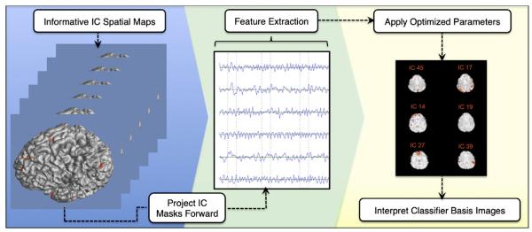
Using a 95% rise threshold, we found that an average of 5.67 +/− 3.26 IC features made up an informative IC feature subset for describing belief and disbelief cognitive states. We therefore selected the top six IC spatial maps from the first two scanning sessions within subject, and then projected these IC masks to the third motion corrected functional scans. Thereafter, the time series were extracted from each of these scans and classification proceeded as described above (Fig. 6) keeping all previously-optimized hyperparameters fixed. Performance accuracy diminished by 8.2% for J48 decision tree.

Fig. 6.

Methodology for projecting highly ranked IC spatial maps forward onto.

Discussion

Here we have described a method for unsupervised dimension reduction and feature extraction of event related fMRI data. Dimension reduction was accomplished by performing ICA, and feature extraction proceeded by sampling corresponding IC time courses. Sampled IC timecourses were then used as inputs for training and testing of six different ML classification algorithms with the goal of discriminating between the cognitive states of “belief” and “disbelief” at each test event. Given that a priori knowledge is not required for dimension reduction and feature extraction, the described analysis pipeline may be particularly useful when then goal is exploratory analysis. Our goal was to perform robust classification based on functionally meaningful patterns in neuroimaging data, and to optimize parameters at key steps in the decoding process. In our framework, robustness includes: classification accuracy, stability, interpretability, and generalization capability.

Performance comparison across classifiers

According to the “no free lunch” theorem (Wolpert et al., 1995), there is no single learning algorithm that universally performs best across all domains. As such, a number of classifiers should be tested. Here, the two best performing classifiers were AdaBoost and Random Forest with Random Forest providing the highest overall correct classification. AdaBoost achieved 89% with only four components. Naïve Bayes produced correct classification rates comparable to AdaBoost, but required more ICs to achieve this accuracy, and had several classification rates below 80%. Although SVM performance was not as high as other classifiers tested here, improvements in SVM performance would likely occur with additional optimization of hyperparameters. Future optimization work might include implementation of a cross-validated grid search within the training set to find optimal parameter values.

Although Random Forest performed well, caution should be used when applying any decision tree based classification scheme, as these methods are prone to overfitting when the number of attributes is large. Given enough leaves, a decision tree often can specify all training data with 100% accuracy, given that impurity generally decreases as data becomes more specified. It is often useful to truncate the process by applying a threshold or pruning technique. Although Random Forest classifiers may produce high levels of classification accuracy, generalization of the results often is poor as compared to AdaBoost, and addition of noise to learning subsets has proven useful in increasing model generalization (Breiman, 2001).

In our observations, high performance with few features was achieved with both AdaBoost and Naïve Bayes. In parametric estimation, model parameters are estimated from training data and defined over the entire input space. Thereafter, fixed parameter values are applied to test data instances. Nonparametric models, like K*, can be computationally intensive, requiring multiple operations to calculate the distances from the given input to all of the training instances. Growing Random Forests of trees actually can be faster, because tree growth depends on only a subset of the entire training set. In development of real-time classification systems, computational burden must be considered, and the methods described herein may be useful in selecting classifiers that perform well using a parsimonious feature subset.

Optimal feature subset selection and generalization capability

In the analysis here, we utilized a forward search selection process, adding ICs incrementally based on t-stat ranking. Improvements may be obtained via testing alternative methods for ranking IC features, and more sophisticated search algorithms for finding optimal feature subsets such as genetic algorithms. Automatic labeling of IC noise components (Tohka et al., 2008) may also prove useful in reducing the number of features. Using rise threshold measures in combination with a forward search may prove useful for selecting a parsimonious, diagnostic subset of ICs. Additional stop criterion for forward search including Akaike and information Criterion (Akaike, 1974) may also be tested in future work. It is worth noting that our method of projecting a subset of six features forward generalized well to other scanning sessions within subject as demonstrated here.

Comparison of this method to conventional general linear model analysis

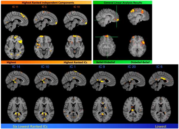
Conventional analysis of fMRI BOLD data involves using model-driven general linear model approaches (Friston et al., 1995) for brain mapping purposes (Poldrack, 2006). We compared our classification method to our previously published GLM results on this same data set. The highest ranked IC spatial maps (Fig. 7a) show similarity to brain regions associated with contrasts for belief–disbelief, and disbelief–belief (Harris et al., 2008). IC spatial maps that were ranked lowest for the same subject trial generally corresponded to noise or artifact, and would generally carry little diagnostic capability in discriminating between belief and disbelief states (Fig. 7b).

Fig. 7.

IC spatial maps of components ranked highest for a certain subject. (a) Comparison of highest ranked IC spatial maps (left) with published GLM results (right). Ventromedial prefrontal cortex activity appears in IC 5 and IC 19, consistent with the belief–disbelief contrast. Superior frontal gyrus and left frontal gyrus activity in IC 11, ranked highest, is similar to the disbelief–belief contrast. All images are shown with the same z-statistic threshold (2.5–3.7). (Harris et al., 2008) (b) IC spatial maps of the six lowest ranked ICs in the same subject, starting with IC 14 (left) and progressing in order to the lowest, IC 6 (right). IC numbers are derived from FSL MELODIC output.

Interpretation of basis images used for classification

When used in neuroscience research, ML results vary widely in their interpretability, and there is a need for transparency in ML methodology (Hanke et al., 2010). It is known, for example, that in many cases the dimension used in classification are either artifact-ridden or non-neural altogether. For example, in a recent study (Anderson et al., 2009) image features that were obviously due to head motion contributed significantly to the classification of schizophrenic vs. normal subjects. While this may contribute appropriately to the clinical diagnostic value, it does little to inform the neuroscientist about the disease. Furthermore, building classifiers based on noise may not be repeatable across scanning sessions. Poldrack et al. (2009) showed that a decision tree formed by unsupervised machine learning was able to generate a meaningful taxonomy of the loading of mental concepts in a variety of more complex cognitive states.

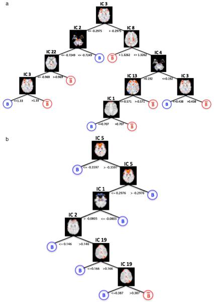
The IC based decoding method presented here can readily be used for interpretation purposes via analysis of the loci of IC basis images used to construct a classifier. For example, AdaBoost weights and nodal hierarchy of ICs used in constructing decision trees (Fig. 8) may represent a basis for describing certain brain states. Interpretation of meta classifiers like Random Forest may prove more challenging given that ICs across numerous trees are used for classification.

Fig. 8.

Structure of J48 decision tree nodal hierarchy for two subjects. IC spatial maps indicate decision nodes. Blue and red circles indicate terminal leaves with discrete outcome labels for belief and disbelief, respectively. Certain IC basis images used for recursive splits have overlap with general linear model contrasts for belief-disbelief and disbelief-belief. For example, in (b), IC 5, used for the initial data split, contains overlap with belief-disbelief contrasts. (For interpretation of the references to colour in this figure legend, the reader is referred to the web version of this article.)

Future considerations

In a recent review (deCharms, 2008) speculated that real-time fMRI classification might find clinical application in neurofeedback-based therapies. Although the current paper is not a real-time paper, it presents a number of optimization and analysis steps that can be useful in a near real-time protocol. The rapid self-paced experimental paradigm used for data collection in this study is not ideal for real-time classification. Changing our stimulus presentation to a rapid serial visual presentation (RSVP) paradigm (Poolman et al., 2008) would minimize saccade artifact while also creating a longer interstimulus interval. This would eliminate the need for sampling only identical consecutive responses when the reaction time for different class labels occurred within a single TR. In the methodology described herein, the most computationally intensive and rate-limiting step is the pICA calculation. To avoid this computational bottleneck, IC spatial maps can be projected forward in time, as demonstrated here. Optimizing this procedure is clearly a topic for future work.

References

- Aha DW. Tolerating noisy, irrelevant and novel attributes in instance-based learning algorithms. Infernat. J. Man-Machine Studies. 1992;36:267–287. [Google Scholar]
- Akaike H. A new look at the statistical model identification. IEEE Trans. Autom. Control. 1974;19:716–723. [Google Scholar]
- Alpaydin E. Introduction to Machine Learning. MIT Press; Cambridge Mass: 2004. [Google Scholar]
- Anderson A, Dinov ID, Sherin JE, Quintana J, Yuille AL, Cohen MS. Classification of spatially unaligned fMRI scans. NeuroImage. 2009 doi: 10.1016/j.neuroimage.2009.08.036. doi:10.1016/j.neuroimage.2009.08.036. [DOI] [PMC free article] [PubMed] [Google Scholar]
- Beckmann CF, Jenkinson M, Woolrich MW, Behrens TEJ, Flitney DE, Devlin JT, et al. Applying FSL to the FIAC data: model-based and model-free analysis of voice and sentence repetition priming. Hum. Brain Mapp. 2006;27(5):380–391. doi: 10.1002/hbm.20246. doi:10.1002/hbm.20246. [DOI] [PMC free article] [PubMed] [Google Scholar]
- Bo TH, Jonassen I. New feature subset selection procedures for classification of expression profiles. Genome Biol. 2002;3(4):1–11. doi: 10.1186/gb-2002-3-4-research0017. [DOI] [PMC free article] [PubMed] [Google Scholar]
- Breiman L. Bagging predictors. Mach. Learn. 1996;24:123–140. [Google Scholar]
- Breiman L. Random Forests. Mach. Learn. 2001;45:5–32. [Google Scholar]
- Budiansky S, Goode EE, Gest T. The cold war experiments. U.S. News & World Report. 1994;116(3):32–34, 36, 38. [PubMed] [Google Scholar]
- Burges C. A tutorial on support vector machines for pattern recognition. Data Min. Knowl. Discov. 1998;2(2):121–167. [Google Scholar]
- Cleary JG, Trigg LE. K*: an instance-based learner using an entropic distance measure. Proceedings of the 12th International Conference on Machine Learning. 1995 [Google Scholar]
- Cox DD, Savoy RL. Functional magnetic resonance imaging (fMRI) “brain reading”: detecting and classifying distributed patterns of fMRI activity in human visual cortex. Neuroimage. 2003;19(2 Pt 1):261–270. doi: 10.1016/s1053-8119(03)00049-1. [DOI] [PubMed] [Google Scholar]
- Corinna C, Vapnik V. Support-Vector Networks. Machine Learning. 1995;20:273–297. [Google Scholar]
- Dash M, Liu H. Feature selection for classification. Int. J. Intell. Data Anal. 1997;1(3) 1997. [Google Scholar]
- deCharms RC. Applications of real-time fMRI. Nat. Rev. Neurosci. 2008;9(9):720–729. doi: 10.1038/nrn2414. doi:10.1038/nrn2414. [DOI] [PubMed] [Google Scholar]
- Douglas PK, Harris S, Cohen MS. Naïve Bayes Classification of Belief verses Disbelief using Event Related Neuroimaging Data. OHBM poster. 2009 [Google Scholar]
- Douglas PK, Harris S, Yuille A, Durnhofer M, Cohen MS. IC Masking for Within Subject Classification Applied to a Bivariate Event Related fMRI task. OHBM poster. 2010 [Google Scholar]
- Friston KJ, Frith CD, Frackowiak RS, Turner R. Characterizing dynamic brain responses with fMRI: a multivariate approach. Neuroimage. 1995;2(2):166–172. doi: 10.1006/nimg.1995.1019. [DOI] [PubMed] [Google Scholar]
- Garrett D, et al. Comparison of linear, nonlinear, and feature selection methods for EEG signal classification. IEEE Trans. Neural Syst. Rehabil. Eng. 2003;11(2) doi: 10.1109/TNSRE.2003.814441. [DOI] [PubMed] [Google Scholar]
- Golub TR, Slonim DK, Tamayo P, Huard C, Gaasenbeek M, Mesirov JP, et al. Molecular classification of cancer: class discovery and class prediction by gene expression monitoring. Science (New York, N.Y.) 1999;286(5439):531–537. doi: 10.1126/science.286.5439.531. [DOI] [PubMed] [Google Scholar]
- Hanson SJ, Matsuka T, Haxby JV. Combinatorial codes in ventral temporal lobe for object recognition: Haxby (2001) revisited: is there a “face” area? Neuroimage. 2004;23(1):156–166. doi: 10.1016/j.neuroimage.2004.05.020. doi:10.1016/j.neuroimage.2004.05.020. [DOI] [PubMed] [Google Scholar]
- Harris S, Sheth SA, Cohen MS. Functional neuroimaging of belief, disbelief, and uncertainty. Ann. Neurol. 2008;63(2):141–147. doi: 10.1002/ana.21301. doi:10.1002/ana.21301. [DOI] [PubMed] [Google Scholar]
- Hart PE. The condensed nearest neighbour rule. IEEE Trans. Inf. Theory. 1968;14:515–516. [Google Scholar]
- Hastie T, Tibshirani R, Friedman J. The Elements of Statistical Learning. Springer Series in Statistics; New York, NY: 2001. [Google Scholar]
- Hanke M, Halchenko YO, Haxby JV, Pollmann S. Statistical learning analysis in neuroscience: aiming for transparency. Front Neurosci. 2010 Apr 15;4:38. doi: 10.3389/neuro.01.007.2010. [DOI] [PMC free article] [PubMed] [Google Scholar]
- Jenkinson M, Bannister P, Brady M, Smith S. Improved optimization for the robust and accurate linear registration and motion correction of brain images. Neuroimage. 2002;17(2):825–841. doi: 10.1016/s1053-8119(02)91132-8. [DOI] [PubMed] [Google Scholar]
- Kohavi R, John G. Wrappers for feature subset selection. Artif. Intell. 1997;97:273–324. [Google Scholar]
- Kriegeskorte N, Goebel R, Bandettini P. Information-based functional brain mapping. Proc. Natl Acad. Sci. USA. 2006;103(10):3863–3868. doi: 10.1073/pnas.0600244103. doi:10.1073/pnas.0600244103. [DOI] [PMC free article] [PubMed] [Google Scholar]
- Kriegeskorte N, Simmons WK, Bellgowan PS, Baker CI. Circular analysis in systems neuroscience: the dangers of double dipping. Nat. Neurosci. 2009 May;12(5):535–540. doi: 10.1038/nn.2303. [DOI] [PMC free article] [PubMed] [Google Scholar]
- LaConte S, Strother S, Cherkassky V, Anderson J, Hu X. Support vector machines for temporal classification of block design fMRI data. Neuroimage. 2005;26(2):317–329. doi: 10.1016/j.neuroimage.2005.01.048. doi:10.1016/j.neuroimage.2005.01.048. [DOI] [PubMed] [Google Scholar]
- LaConte SM, Peltier SJ, Hu XP. Real-time fMRI using brain-state classification. Hum. Brain Mapp. 2007;28(10):1033–1044. doi: 10.1002/hbm.20326. doi:10.1002/hbm.20326. [DOI] [PMC free article] [PubMed] [Google Scholar]
- Liu H, Li J, Wong L. A comparative study on feature selection and classification methods using gene expression profiles and proteomic pattern. Genomic Inform. 2002;13:51–60. [PubMed] [Google Scholar]
- Marquardt D. An algorithm for least-squares estimation of nonlinear parameters. SIAM J. Appl. Math. 1963;11:431–441. [Google Scholar]
- Mourão-Miranda J, Reynaud E, McGlone F, Calvert G, Brammer M. The impact of temporal compression and space selection on SVM analysis of single-subject and multi-subject fMRI data. Neuroimage. 2006;33(4):1055–1065. doi: 10.1016/j.neuroimage.2006.08.016. doi:10.1016/j.neuroimage.2006.08.016. [DOI] [PubMed] [Google Scholar]
- Muller KR, Krauledat M, Dornhege G, Curio G, Blankertz B. Machine learning techniques for brain computer interfaces. Biomed. Technol. 2004;49(1):11–22. [Google Scholar]
- Norman KA, Polyn SM, Detre GJ, Haxby JV. Beyond mind-reading: multivoxel pattern analysis of fMRI data. Trends Cogn. Sci. 2006;10(9):424–430. doi: 10.1016/j.tics.2006.07.005. doi:10.1016/ j.tics.2006.07.005. [DOI] [PubMed] [Google Scholar]
- Pandit M, Kittler J. Feature selection for a DTW-based speaker verification system: Proc. IEEE Internat. Conf. on Acoustic, Speech and Signal Processing (ICASSP) 1998;2:769–773. [Google Scholar]
- Pereira F, Mitchell T, Botvinick M. Machine learning classifiers and fMRI: a tutorial overview. Neuroimage. 2009;45(1 Suppl):S199–S209. doi: 10.1016/j.neuroimage.2008.11.007. doi:10.1016/j.neuroimage.2008.11.007. [DOI] [PMC free article] [PubMed] [Google Scholar]
- Poldrack RA. Can cognitive processes be inferred from neuroimaging data? Trends Cogn. Sci. 2006;10(2):59–63. doi: 10.1016/j.tics.2005.12.004. doi:10.1016/j.tics.2005.12.004. [DOI] [PubMed] [Google Scholar]
- Poldrack RA, Halchenko YO, Hanson SJ. Decodeing the large-scale structure of brain fucntion by classifying mental States across individuals. Nov Psychol. Sci. 2009;20(11):1364–1372. doi: 10.1111/j.1467-9280.2009.02460.x. [DOI] [PMC free article] [PubMed] [Google Scholar]
- Poolman P, Frank RM, Luu P, Pederson SM, Tucker DM. A single-trial analytic framework for EEG analysis and its application to target detection and classification. Neuroimage. 2008 Aug 15;42(2):787–798. doi: 10.1016/j.neuroimage.2008.03.031. [DOI] [PubMed] [Google Scholar]
- Quinlan JR. C4.5: Programs for Machine Learning. Morgan Kaufmann Publishers; San Mateo, CA, US: 1993. [Google Scholar]
- Shannon CE. A Mind-Reading Machine. Bell Laboratories Memorandum. 1953 [Google Scholar]
- Smith SM, Zhang Y, Jenkinson M, Chen J, Matthews PM, Federico A, et al. Accurate, robust, and automated longitudinal and cross-sectional brain change analysis. Neuroimage. 2002;17(1):479–489. doi: 10.1006/nimg.2002.1040. [DOI] [PubMed] [Google Scholar]
- Strother S, La Conte S, Hansen LK, Anderson J, Zhang J, Rottenberg D, Pulapura S. Optimizing the fMRI data-processing pipeline using prediction and reproducibility performance metrics: I. A preliminary group analysis. NeuroImage. 2004;23:S196–S207. doi: 10.1016/j.neuroimage.2004.07.022. [DOI] [PubMed] [Google Scholar]
- Theodoridis S, Koutroumbas K. Pattern Recognition. 4th ed. Elsevier Academic Press; Oxford, UK: 2009. [Google Scholar]
- Tohka J, Foerde K, Aron AR, Tom SM, Toga AW, Poldrack RA. Automatic independent component labeling for artifact removal in fMRI. Neuroimage. 2008;39(3):1227–1245. doi: 10.1016/j.neuroimage.2007.10.013. doi:10.1016/j.neuroimage.2007.10.013. [DOI] [PMC free article] [PubMed] [Google Scholar]
- Vapnik V. The Nature of Statistical Learning Theory. 2nd ed. Springer; New York: 2000. [Google Scholar]
- Viola P, Jones M. Rapid object detection using a boosted cascade of simple features. International Conference on Computer Vision and Pattern Recognition. 2001:511–518. [Google Scholar]
- Wolpert DH, Macready WG, David H, William G. No Free Lunch Theorems for Search. Technical Report SFI-TR-95-02-010 (Santa Fe Institute) 1995 [Google Scholar]
- Yamashita O, Sato M, Yoshioka T, Tong F, Kamitani Y. Sparse estimation automatically selects voxels relevant for the decoding of fMRI activity patterns. Neuroimage. 2008;42(4):1414–1429. doi: 10.1016/j.neuroimage.2008.05.050. doi:10.1016/j.neuroimage.2008.05.050. [DOI] [PMC free article] [PubMed] [Google Scholar]