Interpreting population pharmacokinetic-pharmacodynamic analyses – a clinical viewpoint

Abstract

The population analysis approach is an important tool for clinical pharmacology in aiding the dose individualization of medicines. However, due to their statistical complexity the clinical utility of population analyses is often overlooked. One of the key reasons to conduct a population analysis is to investigate the potential benefits of individualization of drug dosing based on patient characteristics (termed covariate identification). The purpose of this review is to provide a tool to interpret and extract information from publications that describe population analysis. The target audience is those readers who are aware of population analyses but have not conducted the technical aspects of an analysis themselves. Initially we introduce the general framework of population analysis and work through a simple example with visual plots. We then follow-up with specific details on how to interpret population analyses for the purpose of identifying covariates and how to interpret their likely importance for dose individualization.

Introduction

The primary purpose of population pharmacokinetic (PK) and pharmacokinetic-pharmacodynamic (PKPD) analysis is to individualize drug choice and dosing regimen. In this perspective we consider that dose ranging and dose selection in pre-marketing clinical trials as well as culmination of knowledge to develop a product label are all versions of dose individualization which are not conceptually different from that faced in the clinic. Dose individualization in this setting is therefore an overarching term that accounts for both how dosing requirements vary across individuals as well as an understanding of sources of variability in dose requirements.

Dose individualization is achieved by understanding the onset, magnitude and duration of drug effects that result from a given dose and dosing regimen and how these effects vary over the target population. Readers are referred to our companion review [1] for an introductory discussion on PKPD models.

The population approach we see today arose from the development of the conceptual framework of population analysis in 1972 to 1977 [2, 3]. From 1977 there was a trickle of papers over the next 10 years, until 1985 where there was an exponential growth in publications. The application of population analysis methods to therapeutic problems has led to on-going methodological and software development which in turn has resulted in further and more complex applications.

The first population analysis software application NONMEM (NONlinear Mixed Effects Modeling [4–6]) still accounts for the majority of the literature (Table 1). Readers are referred to other papers that describe the history of software development for population analysis [e.g. 7, 8].

Table 1.

Population analysis software

Software*	Number of publications†	First year indexed on MEDLINE and EMBASE
NONMEM	2456	1980
NPEM (NonParametric Expectation Maximization) or NPAG (NonParametric Adaptive Grid)	139	1991
PPharm	4	1996
WinBUGS or related	27	1998‡
Monolix	30	2007
MCPEM (Monte Carlo Parametric Expectation Maximization)	4	2007

^*Phoenix NLME has been recently released but no publications yet cite use of this software.

^†Only about half of publications on MEDLINE or EMBASE mention the software in the title or abstract.

^‡The first use appears to relate to a nonlinear hierarchical modelling application in SAS.

The discipline of population analysis shares a common history with clinical pharmacology and, importantly, the same fundamental aim. Yet, the results of population analyses are often viewed with scepticism by those not in the field, particularly by practising clinicians [9]. This may be attributed to a perceived lack of relevance to clinical practice, the inaccessible nature of the methodology and the use of complex equations and statistical jargon in published papers. As a result the clinical utility of models that are developed in the population analysis setting is diminished.

Aim

There are many general reviews [e.g. 7, 9–15] and introductory articles [e.g. 16, 17] on population analyses and it is not the intention of this article to emulate those works. The purpose of this review is to provide a tool to interpret and extract information from population PKPD analysis publications. This review is aimed at those readers who have heard about population analyses but have not conducted the technical aspects of an analysis themselves.

What is a population analysis?

In this review, we use the term population analysis (also termed repeated measures modelling, nonlinear mixed effects modelling and nonlinear hierarchical modelling) to refer to a set of statistical techniques that can be used to learn about the average response in a population as well as the variability in response that arises from different sources. We use the term response to refer to any biomarker or event that might be measured clinically. Readers are referred to Pillai [7] for a detailed overview of population analysis. The approach has also been reviewed recently in a model based drug development setting [18] and in relation to modelling vs. non-modelling techniques from a statistical stand point [19].

Population analysis is the application of a model to describe data that arise from more than one individual. The process does not require that each study individual provides sufficient data to characterize completely their own PK or PKPD profile. Population analysis methods allow borrowing of information between individuals to fill in gaps in the PK and PD profiles. In doing so the method allows the use of sparse sampling study designs. The influence of patient characteristics (such as renal function) on the PK or PKPD profile can be quantified from the data set as well as any remaining unexplained variability between patients.

For the purposes of this review, we constructed a PK model for a gentamicin-like drug that incorporates the central elements relevant to a population analysis. This drug displays one compartment model characteristics with a volume of distribution (20 l) and clearance (4 l h^–1) and the dose is administered by intravenous bolus. We used this PK model to simulate plasma concentration–time data for 30 patients who received a single intravenous bolus dose of 420 mg (6 mg kg^–1 for a 70 kg individual), where each patient provided seven blood samples at times 0.25, 0.5, 1, 2, 4, 8 and 12 h following dosing (Figure 1). A population analysis was then conducted on the simulation ‘dataset’.

Figure 1.

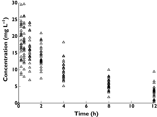
Observed concentration–time data for 30 individuals

A population model for our data will consist of three elements: (1) A model for the typical response – this is the response for a typical (average) patient, (2) a model for heterogeneity and (3) a model for uncertainty.

1.A model for the typical response

This is sometimes also called a structural model. For pharmacokinetics this would be a compartmental model that describes the plasma drug concentration over time (see Figure 2A).

Figure 2.

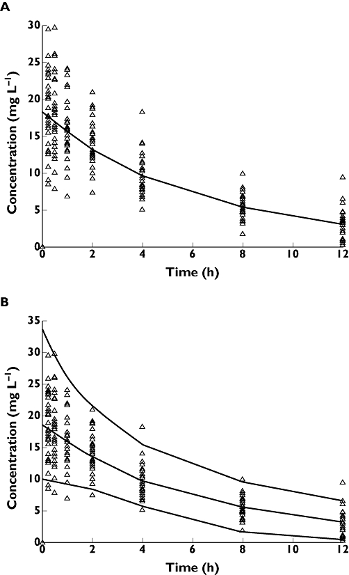
(A) The observed concentration–time data overlaid with the median predicted concentration from the PK model. (B) Observed concentration–time data overlaid with the median and 2.5^th and 97.5^th percentiles of the predicted concentrations from the PK model

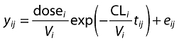
The pharmacokinetic model that describes our gentamicin-like drug at a specific time (t) is:

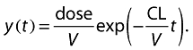(1)

where CL is clearance and V is volume of distribution which will be estimated as a part of the modelling process.

2.A model for heterogeneity

We use the term heterogeneity in population analysis to describe the variability between individuals. This is also termed between subject variability (BSV) or interindividual variability (IIV). This involves two distinct models. Firstly, a model is developed to describe predictable reasons why individuals are different and secondly a model is developed to quantify the remaining source of random variability when we have exhausted our ideas of why individuals are different from one another. The latter model is a statistical model for random variability.

We quantify both predictable and unpredictable variability in a population to characterize not only the typical response of the population, but also to predict the likely range of responses that may occur. In the case of our PK example we now see the range of model predictions in Figure 2B encompass the observed plasma concentration data of our PK example.

If we consider our pharmacokinetic example (Equation 1), we now end up with two equations with Equation 3 directly substituted into Equation 2:

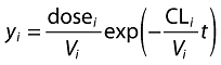(2)

(3)

We use CL_CR as an abbreviation for creatinine clearance and CL_NR as an abbreviation for non-renal clearance. Note that Equation 3 has the same form as simple linear regression (see Figure 3). Here we show a model for renal clearance , where fe = fraction of unchanged drug eliminated by the kidneys (i.e. the slope), and non-renal clearance (i.e. the intercept). We see that CL for the i^th individual is dependent on this individual's CL_CR and non-renal clearance. However, including these processes into Equation 3 is still insufficient to describe completely the variability in CL and hence there is some remaining (residual) variability which we attribute to random variability between patients (the scatter around the regression line in Figure 3). The term c_i is the difference of patient i from the mean patient with this level of renal function and the variance of c over all individuals is the between-subject-variance. We could assume that c is normally distributed, but as shown in Figure 4A this would result in implausible (negative or zero) values of CL. In this particular case, we would consider that c assumes a log-normal distribution which results in no zero or negative values of CL (Figure 4B). A log normal distribution is one in which the natural logarithm transformation of the variable c is normally distributed. The actual value for the difference of any given patient from the average patient is then obtained by exponentiating the value of c.

Figure 3.

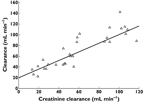
Individual estimates of systemic drug CL vs. creatinine clearance. The line is the regression line and the intercept represents non-renal clearance and the slope represents the fraction of drug cleared unchanged by the kidneys. The vertical difference of any individual from the regression line represents the difference of that individual from the population average and is given by c (Equation 3)

Figure 4.

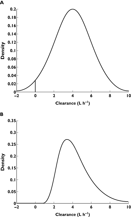
The distribution of values of CL in the population. (A) Allows the distribution to be normal. The verticle line at 0 indicates the lower bound of biologically acceptable values. Here 2.3% of the predicted values of CL are unrealistic. (B) Allows the distribution to be lognormal. Negative (or zero) values of predicted CL are not allowed

We can now show what the predictive plots would look like if we found that CL_CR described 50% of the between-subject variability (heterogeneity) in CL and the remaining 50% of the variability is unexplained (assumed to be random). When we account for CL_CR in the model, we find that the range of model predictions for plasma concentration over time for the 2.5^th and 97.5^th percentiles of the population is now reduced (Figure 5).

Figure 5.

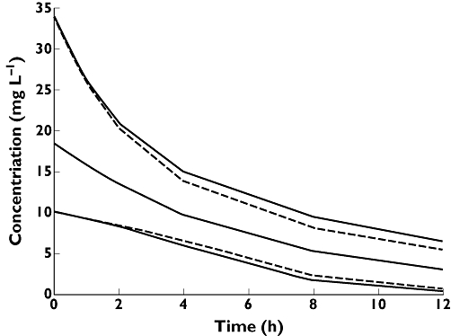
Predicted concentrations from the PK model that does not include the covariate CL_CR (solid line). Predicted concentrations from a PK model that includes the covariate CL_CR as a covariate on CL (dashed lines). Including the covariate CL_CR in the model reduces the unexplained variability in the model predictions and hence improves the reliability of the model predictions

3.A model for uncertainty

This is a statistical model that describes why our models from Equations 1 and 2 do not match our observations exactly. Uncertainty is also called residual error. It is assumed that uncertainty arises from (at least) four sources: (i) process error – where the dose or timing of dose or timing of blood samples are not conducted at the times that they are recorded, (ii) measurement error – where the response (e.g. concentration) is not measured exactly due to assay error, (iii) model misspecification – where the models we propose in Equations 1–3 are in reality too simple and (iv) moment to moment variability within a patient.

The final component to add to our analysis must account for the uncertainty in our model predictions. It is usual, but not essential, to assume that the uncertainty is entirely random and due to error. We can add this into our model by introducing the term e_ij[for error], which is the error for the j^th observation for the i^th individual. We show this for our PK model by

(4)

This error represents the (residual) difference of the model prediction from the data. In the pharmacokinetic example it is usual (but not essential) to consider e to be normally distributed.

Why are population PKPD analyses performed?

To anyone who has performed a population analysis the process is almost as involved and convoluted as the original study that yielded the data. It is therefore sometimes easy to confuse the process and the goal. Population analyses are a useful tool, but not the goal. Here we describe four major reasons why population analyses might be performed. All of these reasons can be related back to either determining that individuals are different, understanding why they are different and accounting for their differences and hence are all globally linked to our notion of the broader picture of dose individualization.

Descriptive population analyses

A descriptive population analysis is used to provide a description of the current data. Although there are a wide range of reasons why this might be performed, two are described here. Firstly, population analyses are often conducted in late phase clinical trials as a method to predict drug exposure (e.g. area under the concentration–time curve) in individuals within the population without the need for intensive sampling from all individuals (see [20]). These predictions are used to examine correlations between safety or efficacy measures and individual exposure. Secondly, a population analysis may simply be conducted to assess which PK or PKPD models best describe the study data. In this case, a series of candidate models are constructed and, using goodness of fit analysis, the model which best agrees with the data is determined (see, for example, Waterhouse et al. [21] for design of an experiment for this purpose and Hennig et al. [22] for the application of the design). In this latter scenario the study would need to be designed to power for appropriate model selection (e.g. see [23]).

Predictive population analyses

Once a population analysis has been completed, simulations from the population model can be used to answer various ‘what-if’ questions. For instance, what dose and dose interval will maximize the ability to achieve a particular therapeutic goal [24, 25], or minimize the occurrence of an adverse effect [26]. There are almost limitless possibilities for ‘what-if’ scenarios and they should be viewed as hypothesis-generating in many cases.

Designing clinical trials

A special case of predictive population analysis is to develop a population PKPD model to perform a sophisticated power analysis to design a future clinical trial (see [27]). This allows ‘what-if’ scenarios to be explored. We have retained designing clinical trials under a separate heading since the rigour required in a population analysis in this setting is generally greater than for a standard population PKPD analysis. In a standard power analysis, the number of subjects can be calculated with knowledge of the size of the difference in treatment effect of clinical interest and the variability in the population. A standard power analysis cannot easily account for the influence of different patient characteristics between the prior study and new study, non-compliance, drop-outs, different dosing regimens and a range of other possible scenarios (see Holford et al. [28] for a recent review).

Identification of covariates

Finally, the identification of covariates is often perceived as the most important clinical output of a population analysis as it provides a basis for dose individualization. A covariate is a patient characteristic which may be phenotypic (e.g. bodyweight or renal function) or genotypic (e.g. CYP2C9 *1*1 for warfarin [29, 30]). Equation 3 provides an example model that might be used to describe the relationship between CL and CL_CR. If a drug has a relatively narrow therapeutic window, and if the relationship between CL and CL_CR is statistically and clinically significant, then correcting for CL_CR will account for heterogeneity in the population and lead to enhanced patient safety.

Interpretation of population analyses

Interpretation and subsequent extraction of information from a population analysis depends on what the clinician wants to learn from the analysis. In the ideal setting the purpose that the reader has will align with the aim of the population analysis. For instance, if the clinician was interested in learning about the influence of covariates then this should be sourced from a report that has this as its primary aim. In this case it is straightforward to extract the information directly from the population analysis.

In circumstances when it is not possible to find a published population analysis that aligns directly with the aims of the clinician, then some critical interpretation of the results may be necessary. Say we are interested in covariate identification. Since this may not have been the primary purpose of the original population analysis then there may not necessarily have been rigorous testing of any covariate relationships that were reported. In this case, we must ask two questions of the reported covariates: (i) was the design appropriate to identify a covariate relationship and (ii) was the covariate relationship significant?

Design of covariate population analyses

The design of population analyses that are used to extract information about covariates can be assessed based on the distribution of covariates in the study population and the number of subjects in the study.

In the former case studying patients with normal renal function will not yield an adequate assessment of renal clearance (i.e. from Equations 2 and 3) even for a drug that is extensively renally cleared. For example, of the seven population analyses for enoxaparin found in a cursory search of the literature, four identified renal clearance as a significant covariate [31–34] while three did not [24, 35, 36], even though the fraction excreted unchanged is approximately 0.8.

In the latter case, if there are too few patients in the study (low power) then the analysis will not be able to identify correctly covariate relationships due to random noise. Hence, low power studies are more likely to find spurious and exaggerated effects. In this regard it is recommended that a minimum of 50 to 100 patients are required to provide accurate estimates of covariate effects in a population analysis setting (readers are referred to Ribbing & Jonsson [37] for a detailed evaluation).

Significance of covariate relationships

For a given population analysis, not all covariates included in the final population model are necessarily significant and not all significant covariates are included in the final population model. This potentially confusing situation requires a means of understanding the significance of any reported covariates. Generally, this can be accomplished by assessing; biological plausibility, clinical significance, statistical significance and a reduction in unexplained between subject variability. It should be noted that the acceptance of a covariate under any one of these criteria does not automatically indicate that the other criteria will also be considered to be true. For instance, it is possible for a covariate to be statistically significant but not clinically significant nor biologically plausible.

Biological plausibility requires that the covariate makes (bio)logical sense, for example CL increases rather than decreases with increasing weight.

Clinical significance implies that the dosing regimen would be modified in accordance with the covariate. For example if only 20% of a drug is eliminated renally, then although creatinine clearance may be included in the model as a statistically significant covariate, it is unlikely that the difference in CL would be significant over a typical range of renal function values and hence this covariate would not be clinically significant.

Statistical significance can be assessed by either global or local tests. Global tests are commonly used and describe the overall fit of the model to the data. When covariates are added to the model then it is expected that the model should provide a better fit to the data. If using NONMEM this is usually assessed by the difference in successive objective function values between the model with the covariate and without the covariate1. A reduction in the objective function by more than 3.84 units (for one added covariate) represents a statistically significant improvement in model fit (P < 0.05). Local tests are aimed at determining the significance of the parameter that describes the covariate relationship. In Equation 3 this is the parameter fe and we would assess its significance by determining whether the confidence interval for fe includes the null value, in this case 0. Confidence intervals can be calculated (asymptotically) using standard methods 95% CI(fe) =fe± 1.96 × SE(fe) where the population analysis report should provide the standard error estimate of fe. It should be noted that global tests and local tests do not always agree, in which case (generally) global tests are preferred.

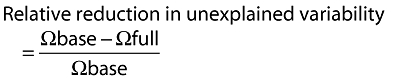
A reduction in unexplained variability implies that dosing based on the covariate value (e.g. dosing based on weight or creatinine clearance) will improve the predictability of the drug effect. To determine a reduction in unexplained variability you need to have access to the variance estimates for the base model and also the full covariate model. The base model is the best model without covariates and the full covariate model is the (best) final model once all covariates have been added into the base model. Unexplained variability between subjects is provided by the remaining between subject variance (based on NONMEM convention we use the symbol Ω for this variance). The difference in the estimated variance of the model parameter in the population (e.g. between subject variance of CL) between the full covariate model and base model provides the potential size of benefit. The relative reduction in variance (Ω) is therefore,

(5)

Note, if the population analysis reports the %CV (percent coefficient of variation) as the measure of between subject variability then the variance can be approximated by Ω≈ (CV%/100)². It is desirable to see a large reduction in the variance (30–50% or more) but this is relatively uncommon and sometimes a modest reduction by 5–10% is reasonable. It is worth noting that not all important and statistically and clinically significant covariates result in a reduction in the unexplained variability. Nevertheless this is a useful guide.

As an example, in the paper by Green & Duffull [24], the aim of this population analysis was to recommend an appropriate individualized dosing regimen for obese patients based on identification of a covariate (lean bodyweight) to predict CL. Here the authors state that lean bodyweight was a significant covariate for CL and total bodyweight for V. The base model is given in table 2 of their text and the full covariate model in table 3 of their text. This was reported as statistically significant using the global goodness of fit measure (the objective function value of NONMEM). We see a significant reduction in the unexplained variability between patients of approximately 30%. Clinical relevance was evaluated by simulating different dosing regimens with and without the covariate of interest and showed the potential clinical utility of dosing based on lean bodyweight as it reduced the probability of excessive concentrations by up to 50%.

Conclusions

In summary, population analysis is a powerful technique that can be used to understand the time course of drug effects. Although these analyses can be statistically complex their application is well-grounded in the principles of clinical pharmacology. These powerful methods provide a method to quantify how well a given dosing regimen will achieve a desirable target and how this dosing regimen can best be modified to meet an individual patient's needs.

Competing Interests

There are no competing interests to declare.

REFERENCES

- 1.Wright DFB, Winter HR, Duffull SB. Understanding the time course of pharmacological effect: a PKPD approach. Br J Clin Pharmacol. 2011;71:815–23. doi: 10.1111/j.1365-2125.2011.03925.x. [DOI] [PMC free article] [PubMed] [Google Scholar]
- 2.Sheiner LB, Rosenberg B, Melmon KL. Modelling of individual pharmacokinetics for computer-aided drug dosage. Comput Biomed Res. 1972;5:411–59. doi: 10.1016/0010-4809(72)90051-1. [DOI] [PubMed] [Google Scholar]
- 3.Sheiner LB, Rosenberg B, Marathe VV. Estimation of population characteristics of pharmacokinetic parameters from routine clinical data. J Pharmacokinet Biopharm. 1977;5:445–79. doi: 10.1007/BF01061728. [DOI] [PubMed] [Google Scholar]
- 4.Sheiner LB, Beal SL. Evaluation of methods for estimating population pharmacokinetic parameters II. Biexponential model and experimental pharmacokinetic data. J Pharmacokinet Biopharm. 1981;9:635–51. doi: 10.1007/BF01061030. [DOI] [PubMed] [Google Scholar]
- 5.Sheiner LB, Beal SL. Evaluation of methods for estimating population pharmacokinetic parameters. III. Monoexponential model: routine clinical pharmacokinetic data. J Pharmacokinet Biopharm. 1983;11:303–19. doi: 10.1007/BF01061870. [DOI] [PubMed] [Google Scholar]
- 6.Sheiner LB, Beal SL. Evaluation of methods for estimating population pharmacokinetic parameters. I. Michaelis-Menten model: routine clinical pharmacokinetic data. J Pharmacokinet Biopharm. 1980;8:553–71. doi: 10.1007/BF01060053. [DOI] [PubMed] [Google Scholar]
- 7.Pillai G, Mentre F, Steimer J-L. Non-linear mixed effects modeling – from methodology and software development to driving implementation in drug development science. J Pharmacokinet Pharmacodyn. 2005;32:161–83. doi: 10.1007/s10928-005-0062-y. [DOI] [PubMed] [Google Scholar]
- 8.Aarons L. Software for population pharmacokinetics and pharmacodynamics. Clin Pharmacokinet. 1999;36:255–64. doi: 10.2165/00003088-199936040-00001. [DOI] [PubMed] [Google Scholar]
- 9.Minto C, Schnider T. Expanding clinical applications of population pharmacodynamic modelling. Br J Clin Pharmacol. 1998;46:321–33. doi: 10.1046/j.1365-2125.1998.00792.x. [DOI] [PMC free article] [PubMed] [Google Scholar]
- 10.Bonate PL. Recommended reading in population pharmacokinetic pharmacodynamics. AAPS J. 2005;7:E363–73. doi: 10.1208/aapsj070237. [DOI] [PMC free article] [PubMed] [Google Scholar]
- 11.Ette EI, Williams PJ. Population pharmacokinetics II: estimation methods. Ann Pharmacother. 2004;38:1907–15. doi: 10.1345/aph.1E259. [DOI] [PubMed] [Google Scholar]
- 12.Ette EI, Williams PJ. Population pharmacokinetics I: background, concepts, and models. Ann Pharmacother. 2004;38:1702–6. doi: 10.1345/aph.1D374. [DOI] [PubMed] [Google Scholar]
- 13.Ette EI, Williams PJ, Lane JR. Population pharmacokinetics III: design, analysis, and application of population pharmacokinetic studies. Ann Pharmacother. 2004;38:2136–44. doi: 10.1345/aph.1E260. [DOI] [PubMed] [Google Scholar]
- 14.Al-Sallami HS, Pavan Kumar VV, Landersdorfer CB, Bulitta JB, Duffull SB. The time course of drug effects. Pharm Stat. 2009;8:176–85. doi: 10.1002/pst.393. [DOI] [PubMed] [Google Scholar]
- 15.Csajka C, Verotta D. Pharmacokinetic-pharmacodynamic modelling: history and perspectives. J Pharmacokinet Pharmacodyn. 2006;33:227–79. doi: 10.1007/s10928-005-9002-0. [DOI] [PubMed] [Google Scholar]
- 16.Schoemaker RC, Cohen AF. Estimating impossible curves using NONMEM. Br J Clin Pharmacol. 1996;42:283–90. doi: 10.1046/j.1365-2125.1996.04231.x. [DOI] [PMC free article] [PubMed] [Google Scholar]
- 17.Wade JR, Edholm M, Salmonson T. A guide for reporting the results of population pharmacokinetic analyses: a Swedish perspective. AAPS Journal. 2005;7:45. doi: 10.1208/aapsj070245. [DOI] [PMC free article] [PubMed] [Google Scholar]
- 18.Grasela TH, Dement CW, Kolterman OG, Fineman MS, Grasela DM, Honig P, Antal EJ, Bjornsson TD, Loh E. Pharmacometrics and the transition to model-based development. Clin Pharmacol Ther. 2007;82:137–42. doi: 10.1038/sj.clpt.6100270. [DOI] [PubMed] [Google Scholar]
- 19.Senn S. Statisticians and pharmacokineticists: what they can still learn from each other. Clin Pharmacol Ther. 2010;88:328–34. doi: 10.1038/clpt.2010.128. [DOI] [PubMed] [Google Scholar]
- 20.Lalonde RL, Kowalski KG, Hutmacher MM, Ewy W, Nichols DJ, Milligan PA, Corrigan BW, Lockwood PA, Marshall SA, Benincosa LJ, Tensfeldt TG, Parivar K, Amantea M, Glue P, Koide H, Miller R. Model-based drug development. Clin Pharmacol Ther. 2007;82:21–32. doi: 10.1038/sj.clpt.6100235. [DOI] [PubMed] [Google Scholar]
- 21.Waterhouse TH, Redmann S, Duffull SB, Eccleston JA. Optimal design for model discrimination and parameter estimation for itraconazole population pharmacokinetics in cystic fibrosis patients. J Pharmacokinet Pharmacodyn. 2005;32:521–45. doi: 10.1007/s10928-005-0026-2. [DOI] [PubMed] [Google Scholar]
- 22.Hennig S, Waterhouse TH, Bell SC, France M, Wainwright CE, Miller H, Charles BG, Duffull SB. A d-optimal designed population pharmacokinetic study of oral itraconazole in adult cystic fibrosis patients. Br J Clin Pharmacol. 2007;63:438–50. doi: 10.1111/j.1365-2125.2006.02778.x. [DOI] [PMC free article] [PubMed] [Google Scholar]
- 23.Roos JF, Kirkpatrick CM, Tett SE, McLachlan AJ, Duffull SB. Development of a sufficient design for estimation of fluconazole pharmacokinetics in people with HIV infection. Br J Clin Pharmacol. 2008;66:455–66. doi: 10.1111/j.1365-2125.2008.03247.x. [DOI] [PMC free article] [PubMed] [Google Scholar]
- 24.Green B, Duffull SB. Development of a dosing strategy for enoxaparin in obese patients. Br J Clin Pharmacol. 2003;56:96–103. doi: 10.1046/j.1365-2125.2003.01849.x. [DOI] [PMC free article] [PubMed] [Google Scholar]
- 25.Mandema JW, Stanski DR. Population pharmacodynamic model for ketorolac analgesia. Clin Pharmacol Ther. 1996;60:619–35. doi: 10.1016/S0009-9236(96)90210-6. [DOI] [PubMed] [Google Scholar]
- 26.Bouillon T, Meineke I, Port R, Hildebrandt R, Gunther K, Gundert-Remy U. Concentration-effect relationship of the positive chronotropic and hypokalaemic effects of fenoterol in healthy women of childbearing age. Eur J Clin Pharmacol. 1996;51:153–60. doi: 10.1007/s002280050177. [DOI] [PubMed] [Google Scholar]
- 27.Jordan P, Goggin T, Pillai G, Steimer J-L, Fotteler B, Gieschke R. Modeling and simulation of clinical trials. 2002. In: Simulation for Designing Clinical Trials: Informa Healthcare.
- 28.Holford N, Ma SC, Ploeger BA. Clinical trial simulation: a review. Clin Pharmacol Ther. 2010;88:166–82. doi: 10.1038/clpt.2010.114. [DOI] [PubMed] [Google Scholar]
- 29.Hamberg AK, Wadelius M, Lindh JD, Dahl ML, Padrini R, Deloukas P, Rane A, Jonsson EN. A pharmacometric model describing the relationship between warfarin dose and INR response with respect to variations in CYP2C9, VKORC1, and age. Clin Pharmacol Ther. 2010;87:727–34. doi: 10.1038/clpt.2010.37. [DOI] [PubMed] [Google Scholar]
- 30.Yuen E, Gueorguieva I, Wise S, Soon D, Aarons L. Ethnic differences in the population pharmacokinetics and pharmacodynamics of warfarin. J Pharmacokinet Pharmacodyn. 2010;37:3–24. doi: 10.1007/s10928-009-9138-4. [DOI] [PubMed] [Google Scholar]
- 31.Feng Y, Green B, Duffull SB, Kane-Gill SL, Bobek MB, Bies RR. Development of a dosage strategy in patients receiving enoxaparin by continuous intravenous infusion using modelling and simulation. Br J Clin Pharmacol. 2006;62:165–76. doi: 10.1111/j.1365-2125.2006.02650.x. [DOI] [PMC free article] [PubMed] [Google Scholar]
- 32.Green B, Greenwood M, Saltissi D, Westhuyzen J, Kluver L, Rowell J, Atherton J. Dosing strategy for enoxaparin in patients with renal impairment presenting with acute coronary syndromes. Br J Clin Pharmacol. 2004;59:281–90. doi: 10.1111/j.1365-2125.2004.02253.x. [DOI] [PMC free article] [PubMed] [Google Scholar]
- 33.Hulot J-S, Vantelon C, Urien S, Bouzamondo A, Mahe I, Ankri A, Montalescot G, Lechat P. Effect of renal function on the pharmacokinetics of enoxaparin and consequences on dose adjustment. Ther Drug Monit. 2004;26:305–10. doi: 10.1097/00007691-200406000-00015. [DOI] [PubMed] [Google Scholar]
- 34.Berges A, Laporte S, Epinat M, Zufferey P, Alamartine E, Tranchand B, Decousus H, Mismetti P, Group PS. Anti-factor Xa activity of enoxaparin administered at prophylactic dosage to patients over 75 years old. Br J Clin Pharmacol. 2007;64:428–38. doi: 10.1111/j.1365-2125.2007.02920.x. [DOI] [PMC free article] [PubMed] [Google Scholar]
- 35.Kane-Gill SL, Feng Y, Bobek MB, Bies RR, Pruchnicki MC, Dasta JF. Administration of enoxaparin by continuous infusion in a naturalistic setting: analysis of renal function and safety. J Clin Pharm Ther. 2005;30:207–13. doi: 10.1111/j.1365-2710.2005.00634.x. [DOI] [PubMed] [Google Scholar]
- 36.O'Brien SH, Lee H, Ritchey AK. Once-daily enoxaparin in pediatric thromboembolism: a dose finding and pharmacodynamics/pharmacokinetics study. J Thromb Haemost. 2007;5:1985–7. doi: 10.1111/j.1538-7836.2007.02624.x. [DOI] [PubMed] [Google Scholar]
- 37.Ribbing J, Jonsson EN. Power, selection bias and predictive performance of the Population Pharmacokinetic Covariate Model. J Pharmacokinet Pharmacodyn. 2004;31:109–34. doi: 10.1023/b:jopa.0000034404.86036.72. [DOI] [PubMed] [Google Scholar]