γH2AX foci as a measure of DNA damage: a computational approach to automatic analysis

Abstract

The γH2AX focus assay represents a fast and sensitive approach for detection of one of the critical types of DNA damage – double-strand breaks (DSB) induced by various cytotoxic agents including ionising radiation. Apart from research applications, the assay has a potential in clinical medicine/pathology, such as assessment of individual radiosensitivity, response to cancer therapies, as well as in biodosimetry. Given that generally there is a direct relationship between numbers of microscopically visualised γH2AX foci and DNA DSB in a cell, the number of foci per nucleus represents the most efficient and informative parameter of the assay. Although computational approaches have been developed for automatic focus counting, the tedious and time consuming manual focus counting still remains the most reliable approach due to limitations of computational approaches.

We suggest a computational approach and associated software for automatic focus counting that minimises these limitations. Our approach, while using standard image processing algorithms, maximises the automation of identification of nuclei/cells in complex images, offers an efficient way to optimise parameters used in the image analysis and counting procedures, optionally invokes additional procedures to deal with variations in intensity of the signal and background in individual images, and provides automatic batch processing of a series of images. We report results of validation studies that demonstrated correlation of manual focus counting with results obtained using our computational algorithm for mouse jejunum touch prints, mouse tongue sections and human blood lymphocytes as well as radiation dose response of γH2AX focus induction for these biological specimens.

1 Introduction

1.1 DNA damage assays in biology and medicine

The realisation of the central role of DNA in biology prompted much interest in developing assays to detect and measure DNA damage. Much of this attention was in the province of radiobiology, driven by the dogma that DNA is the initial molecular target of ionising radiation, but it also extends to drugs and other agents that target DNA. However, the motivation for the effort extended beyond mechanistic studies, especially in the oncology arena, where there is an obvious interest in determining the sensitivity and response of individual patients to radiation and DNA-targeted drugs. Similarly, the possibility of accidental or deliberate exposure to ionising radiation has focussed attention on the need for assays that can provide a retrospective assessment of the radiation dose sustained by individuals after the exposure event; i.e. biodosimetry [1–4].

Whilst there are many types of radiation-induced DNA damage, such as base modification and DNA-DNA and DNA-protein crosslinks, in the radiobiology context, strand breakage and especially DNA double-strand breaks (DSB) are thought to be the most critical. Assays for detection and measurement of DSB are usually based on the isolation of DNA from irradiated cells and DNA size analysis by various separation techniques such as sedimentation, gel electrophoresis, neutral filter elution, and neutral comet assay. The sensitivity and accuracy of these assays is limited with a detection limit being about 5–10 Gy [5–8]. Assays that are based on the cytogenetic methods are much more sensitive with a detection limit about 0.1 Gy, however they detect quite remote consequences of DSB such as micronuclei and chromosome aberrations [9, 10]. The γH2AX assay, described in more detail in the following section, represents a quantum advance in the pathway of DNA DSB assay development. The advance is not just in the sensitivity with a detection limit down to 0.003 Gy [11, 12], but also in the short development time of the endpoint; as little as 30 min post irradiation [13, 14].

1.2 γH2AX foci as an indicator of DNA damage

The γH2AX assay exploits the phosphorylation of the histone variant H2AX (resulting in γH2AX) in response to the induction of DNA DSB [12, 15]. The phosphorylation is initiated at a site of DSB but extends to the adjacent chromatin area [12–15]. This event can be visualised microscopically as a distinct focus within a cell using a fluorescent antibody specific for γH2AX. It is deemed that there is an one-to-one correspondence between DNA DSB and γH2AX focus, therefore the number of γH2AX foci is considered as a measure of the number of DNA DSB [16]. Although the γH2AX foci assay represents an indirect detection of DNA DSB, it has important advantages in comparison to other DSB measurement approaches. First, it measures the number of foci in situ, thus allowing quantitation of the radiation response in individual cells and building the distribution of cells with respect to this response. Second, it provides high DSB detection sensitivity allowing measuring DNA damage within biologically relevant range of radiation doses. γH2AX foci appear in cells in a few minutes following irradiation, their number reaches maximum at 30–60 minutes and than gradually declines in a few hours. Since phosphorylation of H2AX is considered as an important step in signalling and initiation of DNA DSB repair process, the decline in the number of γH2AX foci is believed to reflect the kinetics of DNA DSB repair [12], although in several studies the disappearance of foci is reported to be delayed as compared to DSB repair kinetics [17, 18].

These advantages combined to clearly facilitate demonstration of the radiation bystander effect in microbeam experiments [19–22], but also herald many applications as a routine assay in clinical medicine/pathology, such as assessment of individual radiosensitivity [23, 24], response to cancer therapies, as well as biodosimetry [3]. However all these potential routine applications, with their inherent requirement for high throughput, highlight a limitation of the γH2AX assay. The counting of γH2AX foci in individual nuclei, either at the microscope or at a workstation using a processed image, is extremely tedious and time consuming. This is a problem that must be solved for the assay to translate to its full potential. This paper addresses a possible solution to this problem - automated counting of foci. This solution has particular advantages over an alternative solution; automated measurement of total γH2AX fluorescence per nucleus.

1.3 Computational approaches to γH2AX focus analysis

Although various approaches can be used for the detection and quantitation of γH2AX, such as for example immunoblotting [13, 25] or flow cytometry [25–27], the most informative one is the immunofluorescent staining followed by laser scanning confocal microscopy and subsequent image analysis and counting of the distinct γH2AX foci [28, 29]. The advantage of this approach is that the number of foci per nucleus, in contrast to other approaches (e.g. focus fluorescence intensity), represents a measure that in principle allows comparison of the results for various cells and tissues, and results obtained in different laboratories [17, 18]. The focus counting analysis allows also, apart from measuring the average number of foci per nucleus, the investigation of a range of other valuable parameters, such as for example distribution of cells in the respect of the focus number, fraction of focus free cells, intranuclear distribution of foci, fluorescence intensity and size of individual focus.

Initially, focus counting analysis was performed manually (by eye), which is preferred by some researchers since it provides full visual control over the counting process [16, 30, 31]. However, since manual focus counting analysis is very laborious and time consuming, computer assisted approaches are becoming more widely used. Some of these computational approaches are based on the use of the freely available or commercial image analysis software such as ImageJ [32], NIH Image [33] and its Windows counterpart Scion Image [34], MetaMorph (Molecular Devices Inc, US), HistoLab (Microvision Instruments, France), Image Pro (Media Cybernetics Inc, US), AutoQuantX (Meyer Instruments Inc, US), MetaCyte (MetaSystems GmbH, Germany) These approaches invoke computational algorithms at various stages of analysis, starting from image segmentation and focus identification and ending with calculation of numerous quantitative focus parameters, often including writing of custom macros or plug-ins for execution of specific tasks [35–42]. Other approaches rely on custom software developed for dedicated purpose of focus counting analysis such as for example, a standalone FociCounter [43, 44] or focus counting incorporated into automated high throughput image acquisition and processing platform [43, 45]. Computational approaches substantially increase the productivity of the focus counting analysis and, as claimed by some researchers, are free of the unavoidable operator subjectivity and potential bias of the manual counting analysis.

Despite of these advantages there are however some limitations in the current computational approaches to focus counting analysis. For example, identification of individual nuclei in complex images obtained from biological tissues - sections or touch-prints - still remains a manual operation, thus compromising the efficiency of the automated focus counting analysis [43, 46]. The results of the automated focus counting depend on values of parameters that need to be supplied by the operator [35], however no criteria and recommendations have been developed to justify the choice of particular parameter values.

1.4 The objectives of the study

In this study, we are presenting our computational focus counting algorithm and associated software interface that was developed in an attempt to maximally exploit the advantages of a computational approach and at the same time to overcome or minimise its limitations. Key features of our approach that distinguish it from other approaches include:

• the object splitting algorithm for automatic identification of overlapping and adjacent nuclei/cells in complex images obtained from biological tissues;

• the efficient procedure for optimisation of the main focus counting parameters that is based on an objective definition of a focus as an entity and allows the user to choose parameter values that are optimal for a studied set of images;

• the optional use of additional features that deal with properties of particular image sets such as overlapping foci, variations in average image intensity etc;

• the ability to perform batch processing analysis of multiple images.

We report the results of validation studies with the new program and its application to the analysis of radiation induced γH2AX foci induction in a range of biological specimens.

2 Material and Methods

2.1 Mice irradiation and tissue sampling

Male C3H/HeJ mice (~ 11 weeks old) were obtained from the Animal Resource Centre, Perth, Western Australia. All experiments were carried out with the approval of the Peter MacCallum Cancer Centre Animal Experimentation Ethics Committee. Groups of 3 mice were irradiated using a 137-Caesium source (Gammacell 1000 Elite Irradiator, Nordion International, Ottawa, ON, Canada) at a dose rate of 0.57 Gy/min. Thirty minutes after irradiation, the mice were sacrificed and the tongues were removed and snap frozen in cryo-moulds containing Tissue-Tek O.C.T. compound (Sakura, Finetek, USA) on dry ice. The frozen blocks were stored at −80°C until use. Sections (5 µm) were cut using a Leica CM3050 S Cryostat. The cut sections were placed onto clean, dry slides (Thermoscientific Superfrost Plus, Gerhard Menzel GmbH, Germany) for immunofluorescent staining. Using the same mice, touch-prints were made from a section of jejunum from each animal. Briefly, the jejunum was removed and tapped several times onto a clean, dry microscope slide. This process results in a single layer of jejunal cells being transferred onto the slides for immunofluorescent staining.

2.2 Immunofluorescent staining and image acquisition in mouse tissue samples

Mouse tongue sections and jejunum touch-prints were dried at room temperature (RT) for 1 h and fixed with 2% paraformaldehyde (Sigma-Aldrich, St. Louis, MO) for 20 min at RT. Sections were washed three times for 10 min in PBS, permeabilised in 70% ethanol at −20°C for 60 min and proceeded for immunofluorescent staining immediately or stored at 4°C for a time period of up to 2 weeks.

Following permeabilisation, the slides were washed three times for 10 min in PBS and blocked with 8% BSA (Sigma-Aldrich) in PBS-TT (0.5% Tween 20 (Merck KGaA, Darmstadt, Germany), 0.1% Triton X-100 (Sigma-Aldrich)), for 1 hr at RT.

After blocking, the slides were washed 5 min in PBS-TT and incubated with primary rabbit anti phospho-histone H2AX antibody (clone 2577, Cell Signaling Technology, Danvers, MA) at dilution of 1:200 in PBS-TT for 2 hrs at RT in a humidified chamber, washed three times for 5 min with PBS-TT and incubated with Alexa Fluor 488 goat anti rabbit secondary antibody IgG (H+L) (Invitrogen Australia, Mulgrave, VIC, Australia) diluted at 1:500 in 1% BSA for 1 hr in a humidified chamber. The slides were washed twice with PBS-TT and once with PBS, 5 min each time and mounted with Vectashield mounting medium containing PI (Vector Laboratories, Burlingame, CA). The edges of cover slips were sealed with clear nail polish. The slides were stored at 4°C before image acquisition in the closed container.

Images of γH2AX foci and nuclei were acquired with a confocal laser scanning microscope Olympus FLUOVIEW FV1000 (Olympus, Japan) using a UPlan-Apochromat 63x/1.2 water objective (theoretical horizontal resolution of 0.24 µm). The laser scanning parameters were set to z-stack mode with the Helium-Neon laser at 543 nm, multi ion Argon laser at 488 nm and pinhole size of 135 µm. Optical z-sections were scanned with a 1.5 µm increment through the tissue specimens. The number of acquired optical z-sections varied from 7 to 15 depending on the actual specimen thickness. The scanning speed was set to 4 µs/pixel, and the pixel size to 0.132 µm. The laser/photomultiplier settings were initially adjusted depending on the maximum signal level in the image with highest intensity to avoid saturation of the Alexa 488 signal, and then were kept constant for all images acquired within one experiment. At least two images were taken from different fields of the touch-prints and ventral part sections of the tongue of each of the duplicate slides, resulting in the analysis of more then 50 cells in one section.

2.3 Human lymphocytes

Human whole blood lymphocytes were obtained from the NIH blood bank from paid healthy volunteers who had given written informed consent to participate in an IRB-approved study for the collection of blood samples for in vitro research use. The protocol is designed to protect subjects from research risks as defined in 45CFR46 and to abide by all internal NIH guidelines for human subjects research (protocol number 99-CC-0168). The whole blood samples were irradiated in a ¹³⁷Cs MARK I model irradiator (JL Shepherd & Associates, San Fernando, CA) with 2.4 Gy per min dose rate, or sham-irradiated. The lymphocytes were separated from whole blood and processed as previously described [3, 29]. The lymphocytes were fixed with 2% paraformaldehyde for 20 min at room temperature, washed twice with PBS and cytocentrifuged onto microscope slides. After 15-min rehydration in PBS, the slides were stored in chilled 70% ethanol and processed for immunofluorescent staining. Primary mouse monoclonal anti-γ-H2AX antibody (Abcam, Cambridge, MA) and secondary goat anti-mouse Alexa-488 (Molecular Probes, Eugene, OR) were used. Nuclei were stained with PI. Laser scanning confocal microscopy was performed with a Nikon PCM 2000 (Nikon, Augusta, GA).

2.4 Image analysis algorithm

2.4.1 Outline of the image analysis algorithm

The main objective of the focus counting analysis is to count the number of foci per cell nucleus. In terms of image analysis, it means counting small objects within large objects, assuming that large and small objects are identified from different colour channels of the image. In our studies, nuclei are identified using the red (propidium iodide - PI) or blue (4',6-diamidino-2-phenylindole - DAPI) channels, while foci are imaged using the green (fluorescein isothiocyanate - FITC) channel. Figure 1 represents a flow chart outlining major steps and procedures of our algorithm. The nuclei and foci channels are analysed separately. Following identification of nuclei, an object (nucleus) collection is generated and saved as a file. This collection is used then in the process of focus analysis to assign each focus to a particular nucleus as shown in Figure 1, panel A. For automatic focus counting in a batch of images, a collection of objects (nuclei) is first generated for each image in the batch, and a list of image and nuclei collection files serves as input data for automatic analysis. All steps and procedures for focus analysis as shown in Figure 1, panel A (foci channel) are then invoked automatically for each image in the batch.

Figure 1.

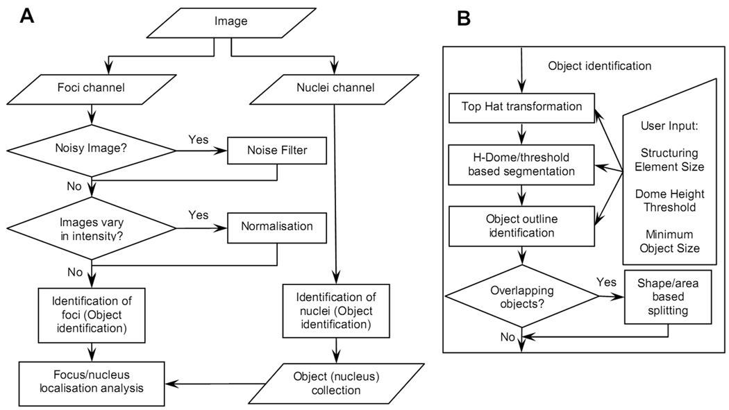
Flow chart demonstrating major procedures involved in the automatic focus counting analysis (panel A) and details of the object identification algorithm (panel B) that is used for identification of both foci and nuclei. An image containing two channels (foci channel and nuclear channel, panel A) represents input data. Each channel is initially analysed separately. For focus identification, optional noise filter and normalisation procedures can be applied if necessary. The focus identification results are analysed in conjunction with the collection of objects (nuclei) generated by the nucleus identification procedure. The object identification procedure (panel B) includes Top Hat transformation to minimise background signal and H-Dome based segmentation in combination with intensity threshold. Four parameters are required as user input: the size of the structuring element, dome height, intensity threshold and minimum object size. The object splitting procedure is applied optionally if overlapping objects are present. For nucleus identification, application of Top Hat transformation and H-Dome based segmentation is optional depending on the origin and quality of the image (nuclei channel).

Given that identification of nuclei and foci are essentially similar tasks, with the only difference being in the size of the object of interest, we applied similar object identification algorithm in both analyses as shown in Figure 1, panel B. In the following section, the term “object” denotes both focus and nucleus.

2.4.2 Major object identification steps and procedures

As the first major step in our object identification algorithm, we applied a classical topological image transformation called Top Hat transformation [35, 47, 48] (Figure 1, panel B). The purpose of the Top Hat transformation in general is to reveal in the image intensity 2D profile some sort of fine structure that is determined by the shape and the size of the so-called structuring element. The transformation efficiently reduces intensity level in those areas of the image where changes in intensity do not fit into the structuring element (background), and leaves unchanged those intensity levels that fit into the structuring element (potential objects). We assumed the structuring element to be a circle, and the size of the structuring element is the first parameter in our algorithm.

Following application of the Top Hat transformation, the segmentation of the resulting image in our algorithm is based on the combination of H-Dome transformation that enables identification of regional maxima [47], and the conventional intensity threshold (Figure 1, panel B). Our combined approach operates with two parameters – the intensity threshold and the dome height that actually determines the regional maxima height as a difference between the peak and valley signal. Such a combined approach allows therefore, on one hand, to separate closely located regional maxima with the valley above the threshold, and on the other hand, to reject those regional maxima that are below the threshold and most likely are the result of the image noise.

Following the image segmentation, an object is defined as a continuous segmented area, and identification and counting of these areas doesn’t represent any difficulties. As a major final step of our object identification algorithm, the minimum object size criterion is applied to reject those objects that are smaller than expected.

In summary, our object identification algorithm requires four parameters the values of which need to be introduced by the operator: the size of the structuring element (related to the maximum object size), the intensity threshold and the dome height (the height of the regional maxima), and the minimum object size.

Our object identification algorithm offers, as an option, application of a procedure that analyses the area and the shape of an object and splits this object into two separate objects, if it doesn’t satisfy the shape/area criteria (Figure 1, panel B). The split path is determined based on the shape of the object outline (presence of a “bottle neck”) and the intensity distribution within the object. Application of this procedure requires two parameters: one that determines the maximum object size and another that determines the acceptable object shape. We use the object roundness as a criterion for the object shape.

2.4.3 Optional procedures for automated focus analysis

The optional application of the noise filter (Figure 1, panel A) that reduces image noise, mainly originating from the equipment (photomultiplier etc), before starting focus analysis can be important. Another optional procedure that improves results of the automatic focus analysis is the normalisation of images. It addresses variations in the intensity of images in a batch and facilitates the use of the same set of counting parameters for all images. Our program offers two ways of normalising images: internal and external normalisation. The internal normalisation assumes multiplication of all pixel intensities by a constant factor as to achieve the effective usage of the full dynamic range offered by a given image format. For the external normalisation, the analysis of the set of images has to be completed first without normalisation, and then the normalisation factor for each image is calculated based on the comparison of the average intensity level for all foci detected in that image. Following normalisation, the counting analysis is then repeated for normalised images.

Although the splitting procedure based on the analysis of the focus size and shape and described in section 2.4.2 substantially improves the results of counting, especially if the number of foci per nucleus is large, it fails to resolve those foci that occupy the same position in a 2D projection, but which are located at different depths. The only approach to resolve such foci is the application of a 3D counting algorithm. Although a true 3D counting algorithm has been suggested for focus counting as a plug in for ImageJ [49], such algorithms require much more processor time and are less suitable for visual inspection, so we chose to employ a pseudo 3D counting in our program. Our algorithm first identifies foci in each z-plane of a stack of images, and then analyses overlapping objects in adjacent z-planes. An object at a given 2D position in the projection image is considered as a single focus if corresponding objects overlap in any two adjacent z-planes. If however at least one z-plane, that is located between z-planes with overlapping objects, does not contain an overlapping object, there are potentially at least two foci at the indicated position.

2.4.4 Nucleus analysis

Depending on the origin and quality of an image, various degrees of automation can be achieved in identification and analysis of nuclei. Automatic nucleus analysis of multiple images using the modified object identification algorithm described in section 2.4.2 (Figure 1, panel B) was employed for images obtained from human blood lymphocytes samples. For such images, Top Hat transformation was excluded from the procedure, and simple intensity threshold was used for image segmentation. For images obtained from tissue samples, the results of nucleus identification achieved using the basic object identification algorithm (Figure 1, panel B) were inspected visually for each image. Since entirely satisfactory splitting of objects can not be achieved for complex images, additional semi-automatic splitting procedures were applied for individual objects by the operator. These were shape/intensity, one-point or two-point splitting procedures, for which the operator specifies one or two points within the object of interest that will belong to the split path. The split path is then computes as a continuous line of pixels based on combination of two criteria: the minimum distance from the split point(s) to the object outline and the minimum signal intensity along the path.

2.5. Focus counting, correlation and regression analysis

Manual and automatic counting were done by different operators, and no results from automatic counting were available for the operator performing manual counting. Results from manual counting were available for the operator performing automatic analysis, however these results were not used for optimisation of major counting parameters, such as the size of structuring element, the dome height and the intensity threshold. Results from manual counting, and in some cases the visual inspection by the manual counting operator, were employed to optimise the minimum focus size and parameters for splitting overlapping foci. For correlation studies, we applied linear regression analysis for automatic versus manual counting data. We calculated the correlation coefficient for the linear regression (R) and presented it as R² (coefficient of determination) which is the fraction of the variance that is explained by the linear regression. The linear regression correlation coefficient corresponds to the Pearson product-moment correlation coefficient. Statistical analysis was done using SigmaPlot for Windows software (Systat Software Inc.).

3 Results

3.1 Automation of identification of nuclei in complex images

We paid a particular attention to automation of identification of nuclei in complex images, since this step is often performed manually even for a computational focus counting analysis [43] or focus count is normalised per total nuclear area in the image [35, 46]. An example of automated identification of overlapped nuclei in an image obtained from a mouse jejunum touch-print is presented in Figure 2. The image shown in panel A was analysed as described in section 2.4.4. Since the majority of nuclei are overlapping, the application of the intensity threshold allows segmentation of nuclear areas as demonstrated in Figure 2, panel B. The subsequent object identification step revealed groups of nuclei that are not separated one from each other as seen in Figure 2, panel C. On the next step, the procedure for object splitting was invoked as described in the section 2.4.2. The results of this application are presented in Figure 2, panel D where object outlines are shown after application of the object splitting procedure with subsequent filtering according to the size and shape of the object. The results clearly demonstrate the ability of the program to automatically separate individual overlapping objects.

Figure 2.

Identification of nuclei in the complex image using object splitting procedure. Panel A shows a fragment of the fluorescent image (DAPI channel, represented as a gray scale image) obtained from a mouse jejunum touch-print. Panel B demonstrates the result of intensity threshold segmentation applied to that image. The segmented area is shown in red colour. Individual nuclei overlap and can not be separated by the intensity threshold segmentation. The outline of the nuclear area is shown in yellow colour in panel C. Pink areas indicate areas below threshold within segmented (nuclear) area. Panel D demonstrates how individual nuclei are automatically separated using our object splitting algorithm. Outlines of individual nuclei are shown in yellow colour.

3.2 Image analysis and focus identification

The application of our image analysis and focus identification algorithm is illustrated in Figure 3. Panel A shows a fragment of an image of mouse tongue section containing two nuclei with nucleus objects outlined in light blue colour. For demonstration purpose, we have chosen objects with quite different level of the signal and background (green channel) to illustrate the capabilities of our algorithm and the role of various steps. Panel D shows the result of the segmentation (shown in dark blue colour) of the green channel using the conventional intensity threshold. It is obvious that the selected intensity threshold, on one hand, is too high to segment focus areas in the top object and, on the other hand, is too low and segments much more than focus area in the bottom object. Application of the Top Hat transformation, as shown in panel B, reduces the background in green channel. Subsequent segmentation based on the combination of H-Dome transformation and the intensity threshold, as shown in panel E, enables segmentation of focus areas in the top object, and at the same time reduces the segmented areas in the bottom object, thus improving separation of potential foci. Panel C shows foci (in yellow colour) identified based on this segmentation. There are however a few overlapping foci that can be automatically separated using the focus splitting procedure as shown in panel F.

Figure 3.

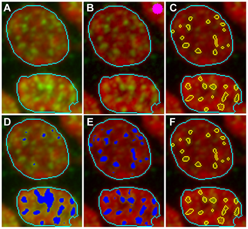
Illustration of the image analysis and focus identification algorithm. Panel A shows a fragment of an image of mouse tongue section with two nucleus object outlined in light blue colour. Panel D shows the segmentation of the image using the conventional intensity threshold. Application of the Top Hat transformation and subsequent segmentation using H-Dome transformation in combination with the intensity threshold are demonstrated in panels B and E respectively. The structuring element is shown in panel B (top left corner) in pink colour. Panel C illustrates identification of foci, and subsequent application of the object splitting procedure is shown in panel F.

3.3 Optimisation of focus counting parameters

Optimisation of the focus counting parameters in our program is based on both visual monitoring of the counting results and the application of a few operator-independent criteria. The optimisation process requires performance of a series of test counting runs with various values of the parameters and to select their optimal combination based on the results of these test runs.

3.3.1 Top Hat and H-Dome transformation parameters

The objective of the optimisation of the Top Hat and H-Dome transformation parameters is to establish values of the size of the structuring element and the dome height that allow revelation and identification of as many as possible foci, so maximisation of the focus count is the optimisation criterion. An example of such optimisation is shown in Figure 4, panel A. We performed a series of test counting runs using various values for the size of the Top Hat structuring element and for the dome height for H-Dome transformation on images that potentially have large number of foci. In the presented example, these were images of lymphocytes obtained from samples of human blood irradiated at 0.6 and 1.5 Gy. Each curve in Figure 4, panel A presents potential focus numbers obtained at various values of the size of the structuring element that are indicated on the horizontal axis, for a fixed value of the dome height. Three such curves were generated for 1.5 Gy image with values of the dome height 40, 50 and 60% (open symbols). The number of detected foci initially increases with increasing size of the structuring element. This increase follows from the fact that, for a small structuring element size, foci that are larger than this size are not scored but regarded as background variations. As the size of the structuring element reaches the maximum focus size (50 – 70 pixels), a plateau or maximum count is reached. Some reduction in focus count is observed with further increase in the size of the structuring element, especially for lower values of the dome height (40–50%). This occurs due to the failure of the H-Dome based segmentation to separate closely located regional maxima (overlapping foci), since for a large structuring element size, clusters of foci are revealed by Top Hat transformation. No reduction in focus count is observed with increasing size of the structuring element for 0.6 Gy image (closed circles in Figure 4, panel A) since overlapping foci are rare in this image. Therefore the size of the structuring element of 50 – 70 pixels and the dome height of 40 – 50% can initially be considered as optimal parameter values. At these values, the maximum focus count is achieved which is not sensitive to the variations of the dome height within the indicated range. However, for 1.5 Gy image overlapped foci are expected, and application of the object splitting procedure results in further increase of focus count with increasing size of the structuring element (closed triangles in Figure 4, panel A). Therefore, the larger size of the structuring element of 140 – 150 pixels should be considered as optimal, that allows identification of focus clusters with subsequent splitting into individual foci. This increased size of the structuring element doesn't influence the focus count in 0.6 Gy image.

Figure 4.

Optimisation of the focus analysis parameters. Each curve in panel A represents results of a series of counting runs using various values of the size of the structuring element (Top Hat transformation) for a fixed value of the dome height (H-Dome transformation) for images from blood lymphocytes samples. Open triangles, squares and inverse triangles represent results for the dome height of 40, 50 and 60% for 1.5 Gy sample. Closed triangles show the result for the dome height 40% following additional application of the object splitting procedure. Open circles represent the results for 0.6 Gy sample and the dome height 40%. Panel B shows the average number of potential foci per nucleus counted at various threshold intensity levels for the control image (non-irradiated sample, circles), test image (5 Gy irradiated sample, triangles) and the difference between the test and control focus count (squares) obtained from mouse tongue sections. The threshold is represented as a percentage of the possible maximum image intensity. An optimal value of the threshold is 3 corresponding to the maximum of the difference between the test and control image.

3.3.2 Intensity threshold parameter

The segmentation of the image in our algorithm is based on a combined approach that uses H-Dome segmentation and the conventional intensity threshold. The main purpose of the conventional threshold is to reject those maxima, that are detected by H-Dome transformation but originate from the image noise. Therefore, optimisation of this parameter is important for the analysis of images with high noise that usually originates from non-specific staining, for example those obtained from tissue sections. An example of the optimisation of the intensity threshold is shown in Figure 4, panel B. Curves in this figure represent potential focus count at various levels of the intensity threshold in mouse tongue sections from the non-irradiated (control) sample (circles), 5 Gy irradiated sample (triangles) and the difference between irradiated and control samples. Obviously, the potential focus count decreases with the increasing intensity threshold, whereas the difference reaches a maximum value and then decreases. Two trends account for the presence of this maximum: at small values of the intensity threshold, the steep decrease in the potential focus count in the control image due to the large contribution of regional maxima originated from the image noise, and at large values of the intensity threshold, the steep decrease in the focus count in the image from irradiated sample due to the rejection of the actual foci. In other words, the maximum is achieved when all potential foci originated from the image noise are rejected and all actual foci are counted. The intensity threshold of 3% that produces this maximum is considered as an optimal value, and this optimisation approach actually defines a focus as an object, the number of which is increased in a test image (with large expected number of foci) as compared to a control image (with small expected number of foci).

The difference in focus count shown in Figure 4, panel B is very sensitive to the value of the intensity threshold and the maximum is well pronounced, therefore the selection of the optimal intensity threshold value (3 % in this case) is critical to obtain valid counting results. The focus counting results, however, are not very sensitive to the value of the intensity threshold for a high intensity/low noise images (data not shown) such as images of blood lymphocytes, for which segmentation is based mainly on H-Dome transformation.

Diagrams as shown in Figure are automatically generated and displayed by our program for quick and efficient optimisation of the size of the structuring element, dome height and intensity threshold parameters. If required, a few iterations of optimising the intensity threshold and Top Hat and H-Dome parameters can be done in turn to refine their values.

3.4 Correlation and radiation dose response studies

We performed a series of analyses that involve parallel counting of foci manually by an operator and automatically using our program. Images were obtained for human blood lymphocytes, mouse jejunum touch-prints and mouse tongue sections. Examples of images used for focus counting analysis are shown in Figure 5. The images are maximum projections of a stack of 8–15 individual z-planes. Three images are presented for each mouse jejunum touch-prints, mouse tongue sections and human blood lymphocytes that were obtained from non irradiated samples and samples irradiated at two different doses. Visual inspection of the images in Figure 5 demonstrates the low level of γH2AX staining in non irradiated samples (panels A, D, G), induction of γH2AX foci in irradiated samples (panels B, E, H) and the increasing number of γH2AX with increasing radiation dose (panels C, F, I). The inserts in the left top corner in panels C, F and I demonstrate identification by our program of individual nuclei and foci within these nuclei.

Figure 5.

Identification and analysis of γH2AX foci in mouse jejunum touch-prints (A, B, C), mouse tongue sections (D, E, F) and human blood lymphocytes. (G, H, I). Images were acquired by confocal laser scanning microscopy from non-irradiated specimens (A, D, G), irradiated with γ-rays at 3 Gy (B, E), 0.6 Gy (H), 5 Gy (C, F) and 1.5 Gy (I). The red channel corresponds to PI staining; the green channel corresponds to γH2AX staining. Examples of nuclei identification and focus automatic identification and counting by our program are shown on inserts in the top left corner of panels C, F and I.

3.4.1 Mouse jejunum touch-prints

Results of γH2AX focus counting in images from mouse jejunum touch-prints are presented in Figure 6. In this experiment, groups of 3 mice were irradiated with radiation doses of 1, 2, 3, 4 and 5 Gy, three jejunum touch-prints from each mouse were prepared and stained for γH2AX immunofluorescence 1 hr after irradiation, and a confocal image was acquired for each touch-print. Each data point in panel A shows the average number of foci per nucleus for an individual image obtained by manual (horizontal axis) and automatic (vertical axis) counting. The analysis indicates a good degree of correlation with the correlation coefficient being R² = 0.799. It should be noted, that apart from the fact that the manual and automatic counting was performed by independent operators, identification of nuclei for each counting approach was also independent. Therefore the extent of observed variations (1 - R² = 0.201) originates from two sources: subjectivity of operators in nuclei identification and differences in automatic versus manual focus counting. The correlation is significantly better when the group average focus numbers obtained by manual and automatic counting are compared as shown in panel B. The correlation coefficient for this case R² = 0.965, and the results of the linear regression indicate that the intercept is not different significantly from 0 (0.125 ± 0.647), and the slope is not different significantly from 1 (0.946 ± 0.090).

Figure 6.

Focus counting analysis in mouse jejunum cells. Mice were irradiated with doses 1, 2, 3, 4 and 5 Gy (3 mice for each dose). Panel A: each data point represents average number of foci per nucleus calculated for an individual fluorescence image. The number of nuclei identified in each image varies from 50 to 160. The total number of images analysed is 47. The line is drawn with the intercept = 0 and the slope = 1. The correlation coefficient R² = 0.799 (P<0.0001). Panel B: each data point represents average number of foci per nucleus calculated in a range of fluorescence images obtained from mouse jejunum touch-prints irradiated at a given dose. Error bars indicate the standard error. The line is generated as a result of linear regression analysis. Two-parameter linear regression analysis resulted in the following values: slope = 0.946 ± 0.090, intercept = 0.125 ± 0.647. Given that the intercept is not different significantly from 0, subsequent single-parameter linear regression resulted in the following value: slope = 0.962 ± 0.036. The correlation coefficient R² = 0.965 (P<0.0005). Panel C: dose response of γ-H2AX foci induction in mouse intestine cells 1 hr after irradiation. Symbols represent results of manual (circles) and automatic (squares) counting. The line is drawn as a result of non-linear regression analysis of combined (manual and automatic) results using the three-parameter saturation model described by the expression: $N(D)=N_0+N_m\left(1-e^{\frac{\delta }{N_m}D}\right)$, where D is the radiation dose, N₀ is the number of foci in non-irradiated cells, N_m is the saturation level, δ [Gy⁻¹] is the focus yield per unit of radiation dose (initial slope of the response curve). The yield of foci δ = 7.5 ± 3.8 Gy⁻¹, the saturation level N_m = 8.06 ± 0.43.

The radiation dose response of the γH2AX focus induction in mouse jejunum cells is presented in Figure 6. Experimental points are shown for manual and automatic focus counting. Results of the non-linear regression analysis using a three-parameter model analysis as described in the Figure 6, panel C legend indicates a substantial deviation from the linear dose response with an obvious trend for saturation at larger doses.

3.4.2 Mouse tongue sections

The correlation study of manual and automatic focus counting in images obtained from mouse tongue sections was carried out in a similar way to that for mouse jejunum touch-prints. The results of γH2AX focus counting in images from mouse tongue sections are presented in Figure 7. In this experiment, groups of 3 or 6 mice were irradiated with doses 0.5, 1, 1.5, 2, 3, 4 and 5 Gy, two sections of mouse tongue were prepared and stained for γH2AX immunofluorescence 1 hr after irradiation, and up to four confocal images were acquired for each section. The correlation coefficients were somewhat higher than those from mouse jejunum studies: R² = 0.886 for correlation of the average foci per nucleus numbers for individual images (panel A) and R² = 0.989 for correlation of the average foci per nucleus number for various radiation dose groups (panel B). The results of the linear regression indicate that the intercept is not different significantly from 0 (0.124 ± 0.308), and the slope is not different significantly from 1 (1.004 ± 0.021).

Figure 7.

Focus counting analysis in mouse tongue basal cells. Mice were irradiated with doses 0.5, 1.0, 1.5, 2, 3, 4 and 5 Gy (3 or 6 mice for each dose). Panel A: each data point represents average number of foci per nucleus calculated for an individual fluorescence image. The number of nuclei identified in each image varies from 50 to 160. The total number of images analysed is 105. The line is drawn with the intercept = 0 and the slope = 1. The correlation coefficient R² = 0.886 (P<0.0001). Panel B: each data point represents average number of foci per nucleus calculated in a range of fluorescence images obtained from mouse tongue sections irradiated at a given dose. Error bars indicate the standard error. The line is generated as a result of linear regression analysis. Two-parameter linear regression analysis resulted in the following values: slope = 0.990 ± 0.042, intercept = 0.124 ± 0.308. Given that the intercept is not different significantly from 0, subsequent single-parameter linear regression resulted in the following value: slope = 1.004 ± 0.021. The correlation coefficient R² = 0.989 (P<0.0001). Panel C: Dose response of γ-H2AX foci induction in mouse tongue basal cells 1 hr after irradiation. Symbols represent results of manual counting (circles), automatic counting (triangles) and automatic 3D counting (squares). Lines show results of non-linear regression analysis using the three-parameter saturation model as described in the Figure 6 legend; solid line for manual and automatic 2D counting, dashed line for automatic 3D counting. The yield of foci for automatic 2D counting δ = 3.05 ± 0.63 Gy⁻¹, for manual counting δ = 3.16 ± 0.42 Gy⁻¹, for automatic 3D counting δ = 4.26 ± 1.20 Gy⁻¹. For manual and automatic 2D counting, the regression analysis reveals some deviation from the linear response with N_m = ~30.

The radiation dose response of the γH2AX focus induction in mouse tongue basal cells is presented in Figure 7, panel C. Three sets of experimental points are shown: the results of manual counting, 2D automatic counting and pseudo 3D automatic counting. For 3D counting analysis, 12 z-planes were analysed for each image as described in the section 2.4.3. Non-linear regression of the manual counting and 2D automatic counting sets using a three parameter model as described in the legend to Figure 6, reveals no significant difference between these two sets and indicates some deviation from the linear dependence. The regression analysis of the 3D counting set results in a 35% increase of γH2AX focus yield as compared to the 2D counting analysis, and suggests the linear dose response. Therefore the deviation of the γH2AX focus dose response from the linear dependence for 2D counting analysis originates from underestimation of focus count due to 3D overlapping foci. This finding is supported by calculation of the probability of focus overlapping. We simulated the random spatial distribution of various focus numbers in a spherical volume, and analysed projections of these foci on the cross-section of this sphere. For nucleus area of 2024 pixels and focus area of 23 pixels (average values calculated from the focus counting analysis), we obtained the expected focus count of 12.8 for 20 simulated foci. These values are of the same magnitude as the results of 2D and 3D counting shown in Figure 6.

3.4.3 Human blood lymphocytes

Blood samples from four donors were used in this study. Samples from three donors were irradiated with a range of doses and stained for γH2AX fluorescence 30 min after irradiation. Samples from one donor were irradiated with a fixed dose of 0.6 Gy and stained at various time intervals after irradiation. Images for the analysis were grouped so that each group represented either one particular radiation dose for a given donor, or one particular fixation time. Manual and automatic counting and calculation of group average values for focus number per nucleus were performed by independent operators. Correlation of these average numbers is shown in Figure 9, panel A with a coefficient R² = 0.973 that indicates a good degree of correlation.

The radiation dose response of the γH2AX focus induction in human lymphocytes obtained from results of the automatic focus counting is shown in Figure 9, panel B. The linear dose response is observed in the range of investigated doses with a statistically significant level of background foci and minor variations between donors in radiation induced focus yield. Figure 9, panel C demonstrates the kinetics of γH2AX following 0.6 Gy irradiation.

4 Discussion

Any computational algorithm designed to identify and count foci operates with a certain number of parameters that need to be specified by the operator. Obviously, algorithms with smaller number of parameters are preferable since they would be less complicated, easier to learn and more user friendly. However, there is a certain minimum number of parameters dictated mainly by the quality and complexity of images. An ideal bi-level image with the level zero signal in the background area and the level one signal in the foci area would not require parameters at all. A real image obtained by using available at present immunofluorescent staining and confocal microscopy technologies features the presence of the background signal and the variation of the signal in the focus area. Segmentation of such images is usually based on the introduction of the intensity threshold parameter that is present explicitly or implied in majority of focus identification algorithms [36, 38]. In our algorithm, the segmentation is dependent, apart from the intensity threshold, on Top Hat and H-Dome transformations, thus adding two more parameters at the segmentation step. This might appear as an over parameterisation of the approach, however it allows to efficiently segment images in cases where simple intensity threshold fails, as for example in images with significant variations in the background level so that it might exceed in some areas the signal level. The application of Top Hat transformation in our algorithm efficiently reduces background in such images as demonstrated in Figure 3. The simple intensity threshold segmentation also fails to separate two or more adjacent objects (potential foci) if the valley (minimum intensity) between these objects is above the threshold. Another disadvantage of the intensity threshold segmentation is that, due to unavoidable variations between images in average intensity, individual threshold values needs to be applied for various images, and some published algorithms suggest calculation of individual threshold for each image [36]. These two issues are resolved in our algorithm by segmentation based on H-Dome transformation as demonstrated in Figure 3.

The results of automated focus analysis are highly dependent on values of the parameters used in a computational approach. Many studies that are based on computational approaches specify the values of these parameters; however they rarely indicate how and why the particular values were used. Meanwhile, the dependence of the counting results on the chosen parameter values raises the issue of what should be considered as a focus [35]. The results of the published study [35] indicates that although the number of automatically counted foci depends on the chosen intensity threshold, the linearity of the dose response is maintained for different threshold values, and therefore it is suggested to use the focus count as a relative measure. This raises the question of how foci counted by automatic procedure relate to those counted manually and invokes criticism of automatic focus counting. To address these issues, the aim of the parameter optimisation in our approach is twofold. On one hand, we introduced the procedure to choose operator-independent values of parameters to define a focus objectively, and on the other hand, we cannot avoid subjectivity and ignore the operator input to achieve the best one-to-one correlation between manual and automatic counting. Values of three major parameters, such the size of structuring element, the dome height and the intensity threshold are determined in our approach using objective criteria – the maximum focus count and the maximum difference between “test” and “control” images. However the value of a parameter such as the minimum focus count, that affects one-to-one correlation of manual and automatic counting, is determined by the operator. Our results however indicate that the degree of correlation expressed as the correlation coefficient, nevertheless, doesn’t depend significantly on the choice of the minimum focus size, thus validating our computational approach and parameter optimisation procedure. The choice of the minimum focus size affects mainly the slope of the linear relationship between manual and automatic counting.

Analysis of focus counting in mouse tongue sections revealed some deviation from the linear dose response (Figure 6), and we suggested that this deviation originates from overlapping foci that cannot be resolved by object splitting algorithm. The application of the 3D counting algorithm generated linear dose response (Figure 6). To support this suggestion, we performed simulation of focus overlapping using approach similar to that suggested by Bocker [39]. We should however note that this approach [39] underestimates the overlap since it simulates the random distribution of foci in a circle representing nucleus. Instead, we simulated the random distribution of foci in a sphere and analysed the overlap of their projections on the cross-section of this sphere. The projections are not distributed randomly in the cross-section, they tend to group in the middle, therefore the chance of overlapping increases. Our simulation results indicated that the difference between 2D and 3D counting results (Figure 6) fits quite well into underestimation of focus count due to overlapping.

Analysis of focus count in human blood lymphocytes using the 2D counting algorithm, however, didn’t show any significant deviation from the linear dose response. This finding suggests, that the role of overlapping foci is less significant in this case. Firstly, it is due to the larger, as compared to the mouse tongue cells, nucleus area/focus area ratio: for lymphocytes 6080/39 = 156, and for mouse tongue cells 2024/23 = 88. Secondly, the larger focus area (39 as compared to 23) allows better recognition of the shape of the overlapping foci by object splitting procedure as described in section 2.4.2.

We have also attempted to apply 3D counting algorithm to the analysis of mouse jejunum samples for which non-linear dose response is observed. We however didn’t observe any change in the results towards improving linearity. This suggests the deviation from the linear dose response in this case is not due to count underestimation at higher radiation doses. A non-linear dose response with a trend to saturation in focus count was observed in tissue samples by other researchers. For example, in mouse skin biopsies [40], a trend to saturation is observed at a dose of 2 Gy 30 min after irradiation. The linear dose response in focus count 10 min after irradiation was reported for mouse intestine in the lower dose range up to 1 Gy [31] with 8 foci/Gy yield, however a dose of 2 Gy was considered in this study at 30 min after irradiation, with 10–11 foci scored thus potentially indicating the deviation from linearity.

Conclusions

The computational approach for automatic focus analysis described in this study and the associated program represent an efficient tool for fast and reliable focus counting analysis. The program maximises the automation of the nuclei identification analysis for complex images from biological tissue that contain overlapping objects. The approach offers an efficient and, to a large extent, user-independent way to optimise parameters used in major image analysis and counting procedures. The optional application of additional algorithms allows to deal with variations in intensity of the signal and background in a set of images and separate overlapping foci. The program also provides automatic batch processing of a series of images. Comparative studies of the results obtained by manual and automatic counting demonstrated a good degree of correlation.

We intend to make our program freely available for scientific community. Although we attempted to design a user-friendly interface, some training or reading of the user manual is necessary for a new user. At present, development of the user manual is in progress.

Figure 8.

Focus counting analysis in human blood lymphocytes. Panel A shows correlation of manual and automatic focus counting. Each data point represents an average for a group of images for either one particular radiation dose for a given donor, or one particular fixation time. Images were obtained from irradiated blood from 4 donors: 0650550 - circles, 0650565 - squares, 0650595 - triangles, 0650711 - inverted triangles. Blood from donors 0650550, 0650565, 0650595 was irradiated with doses 0.02, 0.05, 0.1, 0.2, 0.4, 0.6, 0.8, 1.0, and 1.5 Gy, and lymphocytes were fixed 30 min after irradiation. Blood from donor 0650711 was irradiated with 0.6 Gy, and lymphocytes were fixed 0.5, 1, 2, 4 and 8 hrs after irradiation. Two-parameter linear regression analysis resulted in the following values: slope = 1.02 ± 0.03, intercept = 0.14 ± 0.21. Intercept is not different significantly from 0. The correlation coefficient R² = 0.973 (P<0.0001 for the slope). Panel B shows radiation dose response of γ-H2AX focus induction in human blood lymphocytes 30 min after irradiation for 3 donors 06500550 (circles, solid line), 0650565 (triangles, dash line) and 0650595 (squares, dot line). Symbols represent results of automatic counting; lines are generated by the linear regression analysis. Values for intercept are 0.71 ± 20, 0.84 ± 39 and 0.88 ± 32 for 0650550, 0650565 and 0650595 donors respectively, indicating statistically significant level of background γ-H2AX foci based on the linear model. Values for γ-H2AX focus yield are 11.0 ± 0.3, 9.5 ± 0.6 and 12.0 ± 0.5 Gy⁻¹ for donors as indicated above. Panel C shows kinetics of γ-H2AX after irradiation with 0.6 Gy (donor 0650711).

References

- 1.Cucinotta FA, Durante M. Cancer risk from exposure to galactic cosmic rays: implications for space exploration by human beings. Lancet Oncology. 2006;7:431–435. doi: 10.1016/S1470-2045(06)70695-7. [DOI] [PubMed] [Google Scholar]
- 2.Obe G, Durante M. DNA double strand breaks and chromosomal aberrations. Cytogenet. Genome Res. 2010;128:8–16. doi: 10.1159/000303328. [DOI] [PubMed] [Google Scholar]
- 3.Redon CE, Dickey JS, Bonner WM, Sedelnikova OA. gamma-H2AX as a biomarker of DNA damage induced by ionizing radiation in human peripheral blood lymphocytes and artificial skin. Adv. Space Res. 2009;43:1171–1178. doi: 10.1016/j.asr.2008.10.011. [DOI] [PMC free article] [PubMed] [Google Scholar]
- 4.Kinner A, Wu W, Staudt C, Iliakis G. Gamma-H2AX in recognition and signaling of DNA double-strand breaks in the context of chromatin. Nucleic Acids Res. 2008;36:5678–5694. doi: 10.1093/nar/gkn550. [DOI] [PMC free article] [PubMed] [Google Scholar]
- 5.Wlodek D, Banath J, Olive PL. Comparison between pulsed-field and constant-field gel electrophoresis for measurement of DNA double-strand breaks in irradiated Chinese hamster ovary cells. Int. J. Radiat. Biol. 1991;60:779–790. doi: 10.1080/09553009114552591. [DOI] [PubMed] [Google Scholar]
- 6.Story MD, Mendoza EA, Meyn RE, Tofilon PJ. Pulsed-field gel electrophoretic analysis of DNA double-strand breaks in mammalian cells using photostimulable storage phosphor imaging. Int. J. Radiat. Biol. 1994;65:523–528. doi: 10.1080/09553009414550611. [DOI] [PubMed] [Google Scholar]
- 7.Wojewodzka M, Buraczewska I, Kruszewski M. A modified neutral comet assay: elimination of lysis at high temperature and validation of the assay with anti-single-stranded DNA antibody. Mutat Res. 2002;518:9–20. doi: 10.1016/s1383-5718(02)00070-0. [DOI] [PubMed] [Google Scholar]
- 8.Kohn KW. Principles and practice of DNA filter elution. Pharmacol. Ther. 1991;49:55–77. doi: 10.1016/0163-7258(91)90022-e. [DOI] [PubMed] [Google Scholar]
- 9.Bauchinger M. Quantification of low-level radiation exposure by conventional chromosome aberration analysis. Mutat. Res. 1995;339:177–189. doi: 10.1016/0165-1110(95)90010-1. [DOI] [PubMed] [Google Scholar]
- 10.Edwards AA, Lindholm C, Darroudi F, Stephan G, Romm H, Barquinero J, Barrios L, Caballin MR, Roy L, Whitehouse CA, Tawn EJ, Moquet J, Lloyd DC, Voisin P. Review of translocations detected by FISH for retrospective biological dosimetry applications. Radiat Prot Dosimetry. 2005;113:396–402. doi: 10.1093/rpd/nch452. [DOI] [PubMed] [Google Scholar]
- 11.Lobrich M, Rief N, Kuhne M, Heckmann M, Fleckenstein J, Rube C, Uder M. In vivo formation and repair of DNA double-strand breaks after computed tomography examinations. Proc. Natl. Acad. Sci. USA. 2005;102:8984–8989. doi: 10.1073/pnas.0501895102. [DOI] [PMC free article] [PubMed] [Google Scholar]
- 12.Bonner WM, Redon CE, Dickey JS, Nakamura AJ, Sedelnikova OA, Solier S, Pommier Y. γH2AX and cancer. Nat. Rev. Cancer. 2008;8:957–967. doi: 10.1038/nrc2523. [DOI] [PMC free article] [PubMed] [Google Scholar]
- 13.Rogakou EP, Boon C, Redon C, Bonner WM. Megabase chromatin domains involved in DNA double-strand breaks in vivo. J. Cell Biol. 1999;146:905–916. doi: 10.1083/jcb.146.5.905. [DOI] [PMC free article] [PubMed] [Google Scholar]
- 14.Rogakou EP, Pilch DR, Orr AH, Ivanova VS, Bonner WM. DNA double-stranded breaks induce histone H2AX phosphorylation on serine 139. J. Biol. Chem. 1998;273:5858–5868. doi: 10.1074/jbc.273.10.5858. [DOI] [PubMed] [Google Scholar]
- 15.Sedelnikova OA, Pilch DR, Redon C, Bonner WM. Histone H2AX in DNA damage and repair. Cancer Biol. Ther. 2003;2:233–235. doi: 10.4161/cbt.2.3.373. [DOI] [PubMed] [Google Scholar]
- 16.Sedelnikova OA, Rogakou EP, Panyutin IG, Bonner WM. Quantitative detection of (125)IdU-induced DNA double-strand breaks with gamma-H2AX antibody. Radiat. Res. 2002;158:486–492. doi: 10.1667/0033-7587(2002)158[0486:qdoiid]2.0.co;2. [DOI] [PubMed] [Google Scholar]
- 17.Belyaev IY. Radiation-induced DNA repair foci: spatio-temporal aspects of formation, application for assessment of radiosensitivity and biological dosimetry. Mutat Res. 2010;704:132–141. doi: 10.1016/j.mrrev.2010.01.011. [DOI] [PubMed] [Google Scholar]
- 18.Costes SV, Chiolo I, Pluth JM, Barcellos-Hoff MH, Jakob B. Spatiotemporal characterization of ionizing radiation induced DNA damage foci and their relation to chromatin organization. Mutat Res. 2010;704:78–87. doi: 10.1016/j.mrrev.2009.12.006. [DOI] [PMC free article] [PubMed] [Google Scholar]
- 19.Sokolov MV, Smilenov LB, Hall EJ, Panyutin IG, Bonner WM, Sedelnikova OA. Ionizing radiation induces DNA double-strand breaks in bystander primary human fibroblasts. Oncogene. 2005;24:7257–7265. doi: 10.1038/sj.onc.1208886. [DOI] [PubMed] [Google Scholar]
- 20.Sedelnikova OA, Nakamura A, Kovalchuk O, Koturbash I, Mitchell SA, Marino SA, Brenner DJ, Bonner WM. DNA double-strand breaks form in bystander cells after microbeam irradiation of three-dimensional human tissue models. Cancer Res. 2007;67:4295–4302. doi: 10.1158/0008-5472.CAN-06-4442. [DOI] [PubMed] [Google Scholar]
- 21.Smilenov LB, Hall EJ, Bonner WM, Sedelnikova OA. A microbeam study of DNA double-strand breaks in bystander primary human fibroblasts. Radiat. Prot. Dosimet. 2006;122:256–259. doi: 10.1093/rpd/ncl461. [DOI] [PubMed] [Google Scholar]
- 22.Kovalchuk O, Zemp FJ, Filkowski J, Altamirano A, Dickey JS, Jenkins-Baker G, Marino SA, Brenner DJ, Bonner WM, Sedelnikova OA. microRNAome changes in bystander three-dimensional human tissue models suggest priming of apoptotic pathways. Carcinogenesis. 2010 doi: 10.1093/carcin/bgq119. [DOI] [PMC free article] [PubMed] [Google Scholar]
- 23.Olive PL, Banath JP, Keyes M. Residual gammaH2AX after irradiation of human lymphocytes and monocytes in vitro and its relation to late effects after prostate brachytherapy. Radiother. Oncol. 2008;86:336–346. doi: 10.1016/j.radonc.2007.09.002. [DOI] [PubMed] [Google Scholar]
- 24.Vasireddy RS, Sprung CN, Cempaka NL, Chao M, McKay MJ. H2AX phosphorylation screen of cells from radiosensitive cancer patients reveals a novel DNA double-strand break repair cellular phenotype. Br. J. Cancer. 2010;102:1511–1518. doi: 10.1038/sj.bjc.6605666. [DOI] [PMC free article] [PubMed] [Google Scholar]
- 25.MacPhail SH, Banáth JP, Yu TY, Chu EH, Lambur H, Olive PL. Expression of phosphorylated histone H2AX in cultured cell lines following exposure to X-rays. Int. J. Radiat. Biol. 2003;79:351–358. doi: 10.1080/0955300032000093128. [DOI] [PubMed] [Google Scholar]
- 26.Olive PL, Banath JP. Phosphorylation of histone H2AX as a measure of radiosensitivity. Int. J. Radiat. Oncol. Biol. Phys. 2004;58:331–335. doi: 10.1016/j.ijrobp.2003.09.028. [DOI] [PubMed] [Google Scholar]
- 27.Kataoka Y, Murley JS, Baker KL, Grdina DJ. Relationship between phosphorylated histone H2AX formation and cell survival in human microvascular endothelial cells (HMEC) as a function of ionizing radiation exposure in the presence or absence of thiol-containing drugs. Radiat. Res. 2007;168:106–114. doi: 10.1667/RR0975.1. [DOI] [PMC free article] [PubMed] [Google Scholar]
- 28.Nakamura A, Sedelnikova OA, Redon C, Pilch DR, Sinogeeva NI, Shroff R, Lichten M, Bonner WM. Techniques for gamma-H2AX detection. Methods Enzymol. 2006;409:236–250. doi: 10.1016/S0076-6879(05)09014-2. [DOI] [PubMed] [Google Scholar]
- 29.Sedelnikova OA, Horikawa I, Redon C, Nakamura A, Zimonjic DB, Popescu NC, Bonner WM. Delayed kinetics of DNA double-strand break processing in normal and pathological aging. Aging Cell. 2008;7:89–100. doi: 10.1111/j.1474-9726.2007.00354.x. [DOI] [PubMed] [Google Scholar]
- 30.Rube CE, Dong X, Kuhne M, Fricke A, Kaestner L, Lipp P, Rube C. DNA double-strand break rejoining in complex normal tissues. Int. J. Radiat. Oncol. Biol. Phys. 2008;72:1180–1187. doi: 10.1016/j.ijrobp.2008.07.017. [DOI] [PubMed] [Google Scholar]
- 31.Rube CE, Grudzenski S, Kuhne M, Dong X, Rief N, Lobrich M, Rube C. DNA double-strand break repair of blood lymphocytes and normal tissues analysed in a preclinical mouse model: implications for radiosensitivity testing. Clin. Cancer. Res. 2008;14:6546–6555. doi: 10.1158/1078-0432.CCR-07-5147. [DOI] [PubMed] [Google Scholar]
- 32.Collins TJ. ImageJ for microscopy. BioTechniques. 2007;43:S25–S30. doi: 10.2144/000112517. [DOI] [PubMed] [Google Scholar]
- 33. [last accessed 18/10/2010]; http://rsb.info.nih.gov/nih-image.
- 34. [last accessed 18/10/2010]; http://www.scioncorp.com.
- 35.Qvarnstrom OF, Simonsson M, Johansson KA, Nyman J, Turesson I. DNA double strand break quantification in skin biopsies. Radiother. Oncol. 2004;72:311–317. doi: 10.1016/j.radonc.2004.07.009. [DOI] [PubMed] [Google Scholar]
- 36.Hou YN, Lavaf A, Huang D, Peters S, Huq R, Friedrich V, Rosenstein BS, Kao J. Development of an automated γ-H2AX immunocytochemistry assay. Radiat. Res. 2009;171:360–367. doi: 10.1667/RR1349.1. [DOI] [PubMed] [Google Scholar]
- 37.Roch-Lefevre SH, Mandina T, Voisin P, Gruel G, Gonzalez Mesa JE, Valente M, Bonnesoeur M, Garcia O, Voisin P, Roy L. Quantification of γ-H2AX foci in human lymphocytes: a method for biological dosimetry after ionising radiation exposure. Radiat. Res. 2010;174:185–194. doi: 10.1667/RR1775.1. [DOI] [PubMed] [Google Scholar]
- 38.Cai Z, Vallis KA, Reilly RM. Computational analysis of the number, area and density of γ-H2AX foci in breast cancer cells exposed to (111)In-DTPA-hEGF or γ-rays using Image-J software. Int. J. Radiat. Biol. 2009;85:262–271. doi: 10.1080/09553000902748757. [DOI] [PubMed] [Google Scholar]
- 39.Bocker W, Iliakis G. Computational Methods for analysis of foci: validation for radiation-induced γ-H2AX foci in human cells. Radiat. Res. 2006;165:113–124. doi: 10.1667/rr3486.1. [DOI] [PubMed] [Google Scholar]
- 40.Bhogal N, Kaspler P, Jalali F, Hyrien O, Chen R, Hill RP, Bristow RJ. Late residual γ-H2AX foci in mouse skin are dose responsive and predict radiosensitivity in vivo. Radiat. Res. 2010;173:1–9. doi: 10.1667/RR1851.1. [DOI] [PubMed] [Google Scholar]
- 41.Simonsson M, Qvarnstrom F, Nyman J, Johansson KA, Garmo H, Turesson I. Low-dose hypersensitive gammaH2AX response and infrequent apoptosis in epidermis from radiotherapy patients. Radiother. Oncol. 2008;88:388–397. doi: 10.1016/j.radonc.2008.04.017. [DOI] [PubMed] [Google Scholar]
- 42.Markova E, Schultz N, Belyaev IY. Kinetics and dose-response of residual 53BP1/gamma-H2AX foci: co-localization, relationship with DSB repair and clonogenic survival. Int. J. Radiat. Biol. 2007;83:319–329. doi: 10.1080/09553000601170469. [DOI] [PubMed] [Google Scholar]
- 43.Jucha A, Wegierek-Ciuk A, Koza Z, Lisowska H, Wojcik A, Wojewodzka M, Lankoff A. FociCounter: A freely available PC programme for quantitative and qualitative analysis of gamma-H2AX foci. Mutat. Res. 2010;696:16–20. doi: 10.1016/j.mrgentox.2009.12.004. [DOI] [PubMed] [Google Scholar]
- 44. [last accessed 18/10/2010]; http://focicounter.sourceforge.net.
- 45.Barber PR, Locke RJ, Pierce GP, Rothkamm K, Vojnovic B. Gamma-H2AX foci counting: image processing and control software for high-content screening. Proc SPIE. 2007:6441. [Google Scholar]
- 46.Bhogal N, Jalali F, Bristow RG. Microscopic imaging of DNA repair foci in irradiated normal tissues. Int. J. Radiat. Biol. 2009;85:732–746. doi: 10.1080/09553000902785791. [DOI] [PubMed] [Google Scholar]
- 47.Vincent L. Morphological grayscale reconstruction in image analysis: applications and efficient algorithms. IEEE Transactions on Image Processing. 1993;2:176–201. doi: 10.1109/83.217222. [DOI] [PubMed] [Google Scholar]
- 48.Van Droogenbroeck M, Talbot H. Fast computation of morphological operations with arbitrary structuring elements. Pattern Recog. Lett. 1996;17:1451–1460. [Google Scholar]
- 49. [last accessed 13/12/2010]; http://rsbweb.nih.gov/ij/plugins/foci-picker3d/