Power of genome-wide association studies in the presence of interacting loci

Summary

Though multiple interacting loci are likely involved in the etiology of complex diseases, early genome-wide association studies (GWAS) have depended on the detection of the marginal effects of each locus. Here, we evaluate the power of GWAS in the presence of two linked and potentially associated causal loci for several models of interaction between them and find that interacting loci may give rise to marginal relative risks that are not generally considered in a one-locus model. To derive power under realistic situations, we use empirical data generated by the HapMap ENCODE project for both allele frequencies and LD structure. The power is also evaluated in situations where the causal SNPs may not be genotyped, but rather detected by proxy using a SNP in linkage disequilibrium (LD). A common simplification for such power computations assumes that the sample size necessary to detect the effect at the tSNP is the sample size necessary to detect the causal locus directly divided by the LD measure r² between the two. This assumption, which we call the “proportionality assumption”, is a simplification of the many factors that contribute to the strength of association at a marker, and has recently been criticized as unreasonable [Terwilliger and Hiekkalinna 2006], in particular in the presence of interacting and associated loci. We find that this assumption does not introduce much error in single locus models of disease, but may do so in so in certain two-locus models.

Introduction

Genetic association studies are currently an area of great interest as a tool for studying the genetic basis of human diseases. The association approach, in comparison to genetic linkage studies, has better resolution for the detection of a disease locus, a fact which first made association studies in candidate genes, chosen because of their function or because of their location under linkage peaks, a popular tool for identifying susceptibility alleles. The recent technological progress in SNP genotyping and the availability of resources like the HapMap [2005] have made genome-wide association studies (GWAS) possible. However, aside from the technological feasibility, the power of such a strategy for detecting new susceptibility loci in complex diseases is a key issue. There are many considerations that separate GWAS from association studies in candidate genes: the many thousands SNPs required to efficiently sample the genetic variability of the genome necessarily require a strong correction for multiple testing, large samples are thus necessary to have a chance of detecting the relatively weak signals expected in complex diseases, and risks of subtle hidden population structure are important [Clayton, et al. 2005; Wang, et al. 2005].

Further, though multiple loci are very likely involved in the etiology of complex diseases, the initial applications of the genome-wide association approach have depended on the detection of the marginal effects of each locus. However, complex interactions between loci are likely to be the norm, rather than the exception, in the study of complex diseases [Moore 2003]. Interacting loci need not be different genes or chromosomal regions; both linked and associated loci may contribute to susceptibility to diseases. Ultimately, if we consider any causal polymorphism (rather than an entire gene) as a locus, this situation, known as allelic heterogeneity, has been described in many cases [Cohen, et al. 2004; Hugot, et al. 2001; Li, et al. 2006; Weng, et al. 2005]. For some of them, the effects of particular variants are strong enough to be detected by their marginal effects [Duerr, et al. 2006; Klein, et al. 2005]. However, the variety of models is such that a more systematic power study of GWAS for these models is of interest.

The initial power studies of GWAS considered single locus models, which is equivalent to assuming an independent effect of all causal loci [de Bakker, et al. 2005; Wang, et al. 2005]. Studies of more complex two-locus models have either limited themselves to particular allele frequencies [Howson, et al. 2005] or to unlinked loci [Evans, et al. 2006; Marchini, et al. 2005]. Here, we evaluate the power of GWAS in the presence of linked and potentially associated loci, considering several models of interaction between two causal SNPs. This complements the previous work by adding another layer of biologically relevant complexity to the disease model.

For a given case-control sample size and type I error, the power to detect a given disease model further depends on the allele frequencies of the two causal SNPs, the LD between them and the correction for multiple testing. To derive power under realistic situations, we use empirical data generated by the HapMap ENCODE project [2005] for both allele frequencies and LD structure. For each 2-locus genetic model, we determine an average power to detect the region, considering each pair of alleles in the ENCODE region ENM010 as causal.

In the course of this study, we evaluated the power in situations where the causal SNPs may not be genotyped, but rather its effect detected by proxy using a SNP in linkage disequilibrium (LD) with the causal SNP, referred to as a tagSNP (tSNP). In many previous power and sample size studies, taking this into account has been simple: the sample size necessary to detect an effect at a marker is assumed to be the sample size necessary to detect the effect directly at the causal locus divided by the LD measure r² between the two [Kruglyak 1999; Pritchard and Przeworski 2001; Zondervan and Cardon 2004]. This assumption, which we call the “proportionality assumption”, has made r² the statistic of choice in defining tSNPs and judging the coverage of a set of SNPs. Kruglyak [Kruglyak 1999] proposed a cutoff for a “useful” level of LD between a tSNP and a causal SNP at r²=0.1 based on the proportionality assumption, which would suggest a 10X increase in the sample size needed to detect an effect. Currently, it seems that r² values superior to 0.8 have become the cutoff for “useful” LD [de Bakker, et al. 2005; Pe’er, et al. 2006]. However, the “proportionality assumption” is a simplification of the many factors that contribute to the strength of association at a marker, and has recently been criticized as unreasonable [Terwilliger and Hiekkalinna 2006], in particular in the presence of interacting and associated loci. While evaluating the power of the association using tSNPs, we examine the error introduced by this simplification in models with both one and two associated causal loci.

In what follows, we start by presenting the two-locus power study and examine the error in the power computation introduced by the proportionality assumption afterwards.

Methods and Results

Features of a two-locus disease model

A two-locus disease model can be described with the following genotype relative risk (GRR) matrix:

	A/A	A/a	a/a
B/B	GRRAABB	GRRAaBB	GRRaaBB
B/b	GRRAABb	GRRAaBb	GRRaaBb
b/b	GRRAAbb	GRRAabb	1

where SNP 1 has alleles A and a and SNP 2 has alleles B and b and GRRg_i is the GRR of genotype g_i, as compared to genotype aabb.

For our study, we define four GRR matrices to describe two-locus interactions. These are described in Table 1. We label the models in the following way: in the heterogeneity model, the risk for a two locus genotype corresponds to the highest marginal risk associated with the two corresponding one-locus genotypes. Matrix 1 is an example of this type of model with the same recessive effect of alleles within the two locus. In the epistasis model, the effect of a given SNP is only seen in the presence of a certain genotype or genotypes at the other SNP. Matrix 2 is an example of an epistatic model with a recessive effect of alleles within the two loci. In the additive model, the risk increase due to alleles at one locus is the same for all genotypes at the other locus. Matrix 3 is an example of such an additive model with an additive effect of alleles within the two loci and the same effect of the two loci. Finally, in the multiplicative model, the effect of the two SNPs are independent. Risks at the two loci simply multiply. Matrix 4 is an example of a multiplicative model with an additive effect of alleles within the two loci.

Table 1.

Two-locus Genotype Relative Risk (GRR) matrices used in power calculations

		Genotypes	AA	Aa	aa
1.	Heterogeneity	BB	2	2	2
		Bb	2	1	1
		bb	2	1	1
2.	Epistasis	BB	4	1	1
		Bb	1	1	1
		bb	1	1	1
3.	Additive	BB	3	2.5	2
		Bb	2.5	2	1.5
		bb	2	1.5	1
4.	Multiplicative	BB	4	3	2
		Bb	3	2.25	1.5
		bb	2	1.5	1

The equations for deriving the marginal GRRs at each locus and the sample sizes needed to detect them by single locus association testing are presented in Appendix A. As can be seen from equation (6), the GRR at a given SNP (SNP A, for example) not only depends on the two-locus GRR model, but also on the allele frequencies at both SNP A and SNP B and on the linkage disequilibrium between them. Consequently, a variety of marginal single locus GRR models are associated with each two-locus GRR model.

To illustrate the variation of single-locus GRR models, we present in Table 2 different possible GRRs at a causal locus when the underlying disease model is the twolocus heterogeneity model 1 from Table 1. In this example, the frequency of the causal allele at the first SNP (allele A) is set to 0.05 and the frequency of the SNP allele B and the LD between the two SNPs are allowed to vary, with the constraint that the two causal alleles (A and B) are out of phase (the LD between them is negative, D<0). Under this constraint, the observed single-locus GRR model may be unrelated to the actual underlying disease model. Looking at the extreme case where the frequency of SNP B is 0.7 and D’= 1, we see that GRR_AA = 1.3, while GRR_Aa = 0.65, which implies an apparent protective effect of the heterozygote. In this case, the apparent protective effect is a consequence of the two causal loci being in strong LD with each other.

Table 2.

Marginal GRR at a causal locus A with frequency 0.05, under the 2-locus heterogeneity model 1 of Error! Reference source not found., when the two causal alleles are out of phase. Marginal GRRs are given as a function of both the allele frequency at the other locus (in columns) and of D’ between A and B (in lines). Risks for the locus A are presented in the format GRR_AA/GRR_Aa/GRR_aa.

		Allele Frequency at locus B
		0.1	0.3	0.5	0.7	0.9
D’between loci A and B	0	1.98/1.00/1	1.83/1.00/1	1.60/1.00/1	1.34/1.00/1	1.10/1.00/1
	0.2	1.98/1.00/1	1.83/0.98/1	1.59/0.96/1	1.33/0.93/1	1.09/0.91/1
	0.4	1.98/1.00/1	1.83/0.96/1	1.59/0.91/1	1.32/0.86/1	1.08/0.81/1
	0.6	1.98/0.99/1	1.83/0.95/1	1.58/0.87/1	1.31/0.79/1	1.07/0.72/1
	0.8	1.98/0.99/1	1.82/0.93/1	1.57/0.83/1	1.31/0.72/1	1.06/0.62/1
	1	1.98/0.99/1	1.82/0.91/1	1.57/0.78/1	1.30/0.65/1	1.05/0.53/1

Thus, a simple two-locus model of disease can give rise to marginal relative risks outside of those that would be considered in a single-locus model.

Power to detect a two-locus disease model

We sought to estimate the power of a genome-wide association study in the presence of two potentially associated causal SNPs. The factors that influence the power are: the frequencies of the causal SNPs, the LD between them, the two-locus GRR matrix, and the correction for multiple testing. Further, if tSNPs are used, the power will also depend on their allele frequencies and on the LD between the tSNPs and the causal SNPs.

Because genome-wide association scans do not necessarily seek to directly identify the causal SNP, but rather a region or gene worthy of further inspection, we take, for each “full” model (where a “full” model includes a two-locus GRR model and the allele frequencies and LD of the causal SNPs) the maximum power from the two loci (or from the two tSNPs tagging the two causal loci) as the power to detect the region by single locus testing.

Power of allelic and genotypic association tests was calculated using the formulas given in Appendix A, for the different two-locus GRR models presented in Table 1. To consider a large variety of marginal single locus models for each two-locus GRR model, the data on allele frequencies and LD for the two interacting loci were taken from the empirical data generated by the HapMap ENCODE project. This project provides an exhaustive look at the SNP polymorphisms in ten 500-kb regions in the genome. We use data from the region ENM010 in the European-origin population (CEU), which contains 716 polymorphic SNPs. The ENCODE genotype data was downloaded on 15/2/2006 from the HapMap website (www.hapmap.org). Only independent haplotypes (i.e. from the 60 parents) were used in the analysis. Calculation of linkage disequilibrium was done in Haploview v3.11[Barrett, et al. 2005]. The distribution of allele frequencies and the LD plot for the region are presented in Figure 1 and Figure 2, respectively. The 1,023,880 possible pairs of SNP alleles in ENM010 (four allele combinations for each pair of SNPs) were considered, in turn, as being causal. Consequently, to each two-locus GRR model we attached a distribution of single locus GRRs and a distribution of risk genotype frequencies reflecting both the frequency and LD distributions of all SNP allele pairs. Median and ranges of single locus GRR distributions arising from the four two-locus GRR models are presented in Table 3.

Figure 1.

Distribution of minor allele frequencies in ENM010. There are 716 polymorphic SNPs in this region in the sample.

Figure 2.

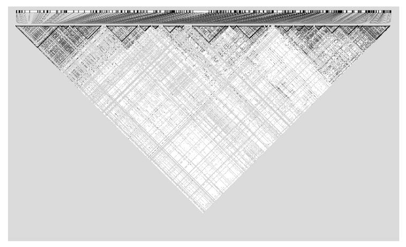
LD plot for the ENCODE region ENM010 generated in Haploview. Black squares represent SNPs in strong LD.

Table 3.

Median and range of single locus GRRs computed from the ENM010 data for different two-locus models. The first number is the median in all two-way models, and the 95% range is presented in brackets. GRR_aa is always one.

Penetrance model	GRRaa	GRRAa
1 (heterogeneity)	1.6 [1, 2]	1 [0.5, 1.2]
2 (epistasis)	1.75 [1, 4]	1 [1, 1]
3 (multiplicative)	2 [1, 4]	1.5 [1.25, 2.25]
4 (additive)	1.66 [1, 3]	1.33 [1, 2]

The ENCODE data were also used to compare the power of different tagging strategies. First, for each tagging strategy (defined by a value of r2 and a minor allele frequency threshold for the SNPs to be tagged), a tSNP was attached as a proxy to each of the 716 SNPs of the ENM010 region, using Tagger [de Bakker, et al. 2005] in Haploview. For each 2-locus “full” genetic model, the power was computed for the two tSNP proxies for the SNP pair that was causal in this “full” genetic model, using the formulas provided in the Appendix A. Second, to compare the power of different tagging strategy (including no tagging at all when all SNPs are tested), specific multiple testing corrections were derived for each strategy, including no tagging at all. To do so, the number of independent tSNPs (or “effective” number of tSNPs) for a whole genome scan were extrapolated from computation based on the 10 ENCODE region data. As the ENCODE data only represent a discrete sampling of 500kb regions on the genome, simply multiplying the mean number of tSNPs necessary in these 10 regions by the number of 500kb blocks on the genome would not properly account for the redundancy of adjacent regions. To do so, we proceeded as follows.

For any tagging strategy, let the number of tSNPs in a given 500-kb region be N₀. Let the number of tSNPs selected using only the first 250-kb block and only the second 250-kb block be N₁ and N₂, respectively. N₀ will always be less than or equal to N₁ + N₂ because of the redundancy removed when the region is divided in half, though the precise difference will depend on the LD structure in the region. We assume that the average amount of redundancy lost by splitting each of the 10 ENCODE regions will be a rough estimate of the redundancy lost by taking any discrete sample of the genome. Among the N₀, N₁ and N₂ SNPs, let the “effective” number of SNPs calculated using the method of Li and Ji[Li and Ji 2005] in each region be M₀, M₁, and M₂. Once again, M₀ will always be less than or equal to M₁ + M₂. Let the difference between the M₀ and (M₁ + M₂) be C. If the size of the genome in kilobases is Gsize (which we let be 3,059,200), then an estimation of the effective number of SNPs on the whole genome, T, is

$$T=\frac{\mathit{Gsize}}{500}\ast {\overline{M}}_0-\left(\frac{\mathit{Gsize}}{500}-1\right)\overline{C}$$

where the bars represent the mean of the given value over the ten 500-kb regions available. The effective number of SNPs corresponds to the number of independent tests and can then be used in a Bonferroni correction. The effective number of tests for a whole genome search corresponding to different tagging strategies are presented in Table 4.

Table 4.

Estimated numbers of tSNPs to cover the entire genome using different tagging parameters and estimated numbers of independent tests (“effective” numbers of SNPs) that they entail.

	Estimated number of
Tagging Parameters	tSNPs	Independent tests
No tagging	6,056,604	992,296
r2=0.8, MAF=0.1	597,770	328,805
r2=0.8, MAF=0.2	385,461	242,475
r2=0.6, MAF=0.1	394,648	217,572
r2=0.6, MAF=0.2	257,586	160,181

Figure 3 shows for the four two-locus GRR models, the percentage of “full” genetic models for which association is detectable as a function of sample sizes, with 80% power and a 5% corrected type I error. The calculations were done using both the one degree of freedom allelic test for association and the two degree of freedom genotypic test for association. Curves are shown for two strategies: no tagging and tagging with parameters r² = 0.8 and MAF = 0.1. In all four 2-locus GRR models considered in this study, the difference between the two tagging strategies and the two tests (genotypic and allelic) is minimal. Overall, the proportion of detectable models is remarkably low. With 5000 individuals, a maximum proportion of 60% is observed and it is for the multiplicative two-locus model. For both epistasis and heterogeneity models, if about 45% of the models are detectable with 4000 individuals, the proportion only weakly increases with increasing sample size. Even with 10,000 individuals, only slightly more than 50% of the models, at best, are detectable. For the additive model, the proportion is smaller than 50% unless samples of 9000 individuals are considered. These three two-locus GRR models generate a high proportion of “full” genetic models that are not detected with single locus association test in conceivable sample sizes. The multiplicative two-locus GRR model is the least sensitive to the SNP frequency and LD distributions, provided that samples large enough are used. With samples of 10,000 individuals, more than 80% of the models are detectable. This multiplicative model also corresponds to the highest mean marginal ORs over all corresponding “full” 2-locus models (see Table 3)

Figure 3.

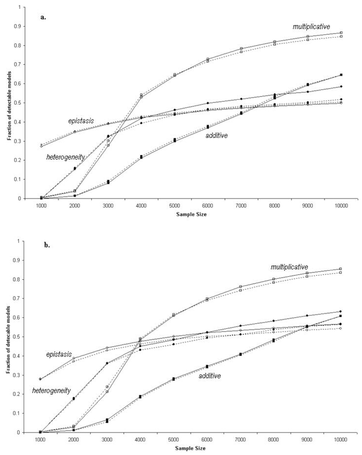
Fraction of detectable models in the ENM010 region under different two-locus models. The solid and dotted lines represent the curves for direct testing and the use of tSNPs, respectively. The filled circles, open circles, filled squares, and open squares represent models 1 (heterogeneity), 2 (epistasis), 3 (additive), and 4 (multiplicative ) respectively. a. using a 1-dof allelic test for association and b. using a 2-dof genotypic test for association.

To illustrate the impact of the marginal frequency distribution of the causal SNPs on the power to detect the different two-locus GRR models, we fixed the sample size at 5000 (2500 cases and 2500 controls) and asked which alleles are detected. In Figure 4, we show the percentage of “full” models that are detectable as a function of the allele frequency of the first causal allele. Once again, the difference between not tagging and tagging is minimal. For the multiplicative two-locus model, most of the models involving alleles with a frequency between 0.15 and 0.75, are detectable. The severe drops at both sides of the frequency scale reflect situations where the risk alleles are either too rare or too frequent for reasonable power of marginal association tests. The pattern is very similar for the additive model though the range of frequencies with a reasonable proportion (around 50%) of detectable models is only between 0.2 and 0.7. The pattern is slightly different for the epistasis and heterogeneity models that are clearly asymmetrical. Only models involving alleles with a minimum frequency of at least 0.5 and 0.3 for heterogeneity and epistasis, respectively, have a reasonable detection proportion (around 50%). Alleles with frequency as high as 0.90 still have the same detection proportion. This reflects the fact that these two models have a recessive effect. Unless risk alleles have a moderate frequency, homozygous at-risk genotypes are too rare to allow detection of the association.

Figure 4.

Fraction of detectable models using the allelic test for association in the ENM010 region as a function of the allele frequency of SNP1 under 4 two-locus GRR models. The solid and dotted lines represent the curves for direct testing and the use of tSNPs, respectively. The filled circles, open circles, filled squares, and open squares represent models 1 (heterogeneity), 2 (epistasis), 3 (additive), and 4 (multiplicative ) respectively.

Error in the proportionality assumption

In the course of doing the above power study, we examined the best way to determine the power to detect an association using a marker associated with a causal locus, rather than a directly genotyped causal locus. The power of a test for association at a genotyped tSNP in linkage disequilibrium with an ungenotyped causal allele is a function of the disease model, the allele frequencies of both the tSNP and the causal SNP, and the LD between the two, as can be seen from Equation (5) of Appendix A. However, the relationship is commonly simplified as N₂ = N₁/r², where N₂ is the sample size (the total combined number of cases and controls) needed to detect the effect by proxy at the tSNP, N₁ is the sample size needed to detect the effect directly at the causal SNP, and r² is the measure of LD between the two loci in the general population. We call this the proportionality assumption, which was made explicit by Pritchard and Pzreworski [Pritchard and Przeworski 2001].

In Appendix B, we highlight one of the assumptions underlying this demonstration: the allele frequencies of both the tSNP and the causal SNP are the same in the general population as in the combined sample of cases and controls. While this is generally true in a prospective study design or a QTL study, in a case-control study the cases are enriched for the causal allele, and thus, the proportionality assumption will only hold if there is no association between the allele tested and the disease. The difference in allele frequencies due to an association may also imply a difference in LD between the combined sample and the general population, as r² is sensitive to allele frequency. If the r² in the sample is greater than r² in the general population, the simplification will overestimate the sample size necessary to detect the association. In the opposite case, the proportionality assumption will underestimate the sample size necessary to detect the association.

The factors that determine the precise error in the proportionality assumption are the allele frequency of the causal allele, the allele frequency of the tSNP, the LD (as measured by D’) between them, and the disease model. We define the error as ε = (N_EXP-N_OBS)/N_EXP, where N_EXP is the estimated sample size needed to detect the effect of the causal allele with a tSNP using the proportionality assumption and N_OBS is the estimated sample size without this assumption, using Equation (7).

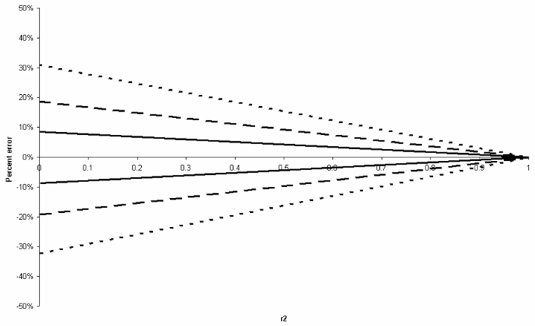
We started by examining the impact of different one-locus disease models on the error in the proportionality assumption. Figure 5-Figure 8 display for 4 genetic models (dominant, recessive, additive and multiplicative), the upper and lower bounds on the error of the allelic association test, for all possible values of LD and all possible allele frequencies at both the tSNP and the causal SNP, summarized by r². Thus, in this figure, a given r² value may correspond to a variety of different LD and allele frequency settings. For GRR smaller than 1.5 and in the absence of other causal alleles, the error in the proportionality assumption is around −20% to 20%. This error, however, is smaller for higher values of r², with error values around −5% to 5% for r² > 0.8.

Figure 5.

Upper and lower bounds on the error in the proportionality assumption for the 1df association test under a one-locus recessive model, where GRR(AA)=× and GRR(Aa)=GRR(aa)=1. Errors are plotted as a function of r2 between the tSNP and the causal SNP. Dotted, dashed and bold lines represent the bounds for ×=5, 2, and 1.5, respectively.

Figure 8.

Upper and lower bounds on the proportionality assumption under for the 1df association test a one-locus multiplicative model, where GRR(AA)= ×2, GRR(Aa)=×, and GRR(aa)=1. Errors are plotted as a function of r2 between the tSNP and the causal SNP. Dotted, dashed and bold lines represent the bounds for ×=2,1.5, and 1.2, respectively.

The presence of an additional causal locus in the region may lead to the violation of another hypothesis underlying the proportionality assumption, which states that the frequencies at the tSNP are independent from the disease status conditional on the causal allele. Indeed, if the tSNP is associated to two causal loci – a plausible situation in our two-locus model- this assumption is violated. This has been highlighted by Terwilliger and Hiekkalinna [Terwilliger and Hiekkalinna 2006], who provide an example in which this non independence leads to the extreme case where either of the two causal alleles would be detected if assayed directly, but neither is detected by proxy, even though r² between one causal SNP and the tSNP is 0.33 (a situation where the detection should be possible at the tSNP providing a three-fold increase of the sample size, according to the proportionality assumption). Because their example presents only a single case, in which the LD between the causal SNP and the tSNP is a fairly weak correlation, we take a more extensive look at this issue.

Following Terwilliger and Hiekkalinna [Terwilliger and Hiekkalinna 2006], assume we have two causal SNPs, A and B, and a tSNP C that tags A. First, if there is no LD between A and B, then the power to detect an association at C is entirely dependant on the relationship between A and C. Second, if the disease alleles A and B are in phase, the interaction will either have no effect or increase power; that is, the relative risks at C may be increased due to the additional effect of allele B. Third, if A and B are out of phase (D<0), it is possible that the interaction may confound the ability to detect an effect. To examine this effect, we consider a situation where there is no ancestral recombination in the region (that is, at most three haplotypes are observed for each two locus combination). We let the mode of interaction between A and B be heterogeneity (see Table 1) and we examine the error in the proportionality assumption as a function of r² between loci A and C. In this framework, an error of −∞ means that the allele is undetectable using a tSNP. Results are presented in Figure 9, in two different frequency settings for the two out of phase causal alleles : the two causal alleles have different frequencies in Figure 9a, while in Figure 9b, the two causal alleles have the same frequencies. If the frequency of C is less than that of A, the proportionality assumption always holds. However, if the frequency of allele C is greater than that of allele A (which it tags), the sample size necessary to detect an effect may be greatly misestimated, even for high values of r².

Figure 9.

Error in the proportionality assumption for the 1df association test for a twolocus heterogeneity model where the causal alleles are out of phase, as a function of r2 between the tSNP and the causal allele it is intended to tag. The bold and dotted portions represent the cases where the frequency of the tag allele is greater than or less than, respectively, the frequency of the causal allele it is intended to tag. a. For the black line, the tSNP tags an allele of frequency 0.1 in the presence of another causal allele of frequency 0.25. The reverse is true for the grey line. b. Both causal alleles have the same frequency. The grey and black lines represent allele frequencies of 0.1 and 0.25, respectively.

To evaluate more exhaustively the impact of two-locus models on the deviation from the proportionality assumption, we computed the error for all “full” 2 locus-models based on the ENM010 data and tSNPs, considering the set of tSNP selected with r² = 0.8 and MAF= 0.1. By construction, this set of tSNP has a r²=0.8 only for the SNPs with a MAF>0.1. For all other SNPs in the region, no constraint is set on r².We could thus assess the impact for a relatively wide range of r². This was done for each of the four two-locus models. Figure 10 presents, by bins of r², the median errors and the 90% ranges calculated in each bin. The median error ranges around −20 /+20 % for all disease models and r² values. However, even with r²=0.8, situations of strong errors are observed, in particular for the heterogeneity and epistasis models.

Figure 10.

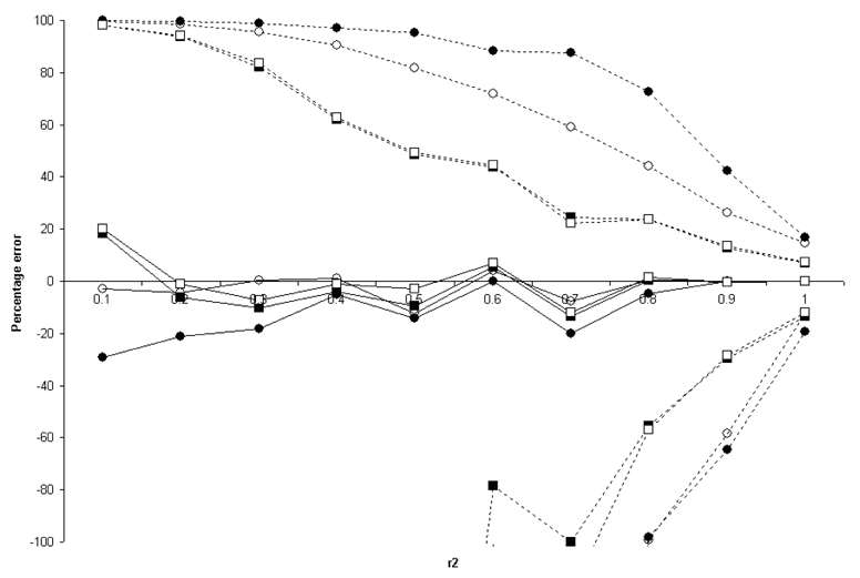
Median (bold) and 90% range (dotted) errors in the proportionality assumption for the two-locus GRR models based on the ENM010 data. The error in each model is binned according to the r2 between the tSNP and one of the causal SNPs. The filled circles, open circles, filled squares, and open squares represent models 1 (heterogeneity), 2 (epistasis), 3 (additive), and 4 (multiplicative ) respectively. The lines do not all converge at r2=1 because the bin labelled 1 contains all the r2 values from 0.9 to 1.

Discussion

The resources and technology necessary for GWAS are now available. The effectiveness of the approach in the presence of multiple interacting susceptibility loci, as are expected in complex diseases, is contingent on the detection of the marginal effect at each locus. For this reason, many previously published GWAS power studies focused on single gene models, arguing that multiple loci models would only result in weakened marginal effects.

However, even simple parameters can give rise to marginal relative risks that are not normally considered in a one-locus model. Further, as outlined by Terwilliger and Hiekkalinna [Terwilliger and Hiekkalinna 2006], the presence of two associated causal loci may impact the power of tSNP based strategies.

In the present study, we evaluated the impact of two locus models on the power of GWAS, and we considered the possibility that the two causal loci are associated. By basing our power study on the HapMap ENCODE data, we measured the impact of a large spectrum of two-locus frequency and linkage disequilibrium patterns on power, including the power of realistic tagging strategies.

There has been much debate over the likely frequencies of causal alleles in complex diseases [Lohmueller, et al. 2003; Pritchard 2001; Pritchard and Cox 2002; Reich and Lander 2001]. Because the debate is not resolved, we chose to base our study on the largest set of two-locus allele frequencies and LD patterns. Therefore, we considered each SNP in the ENM010 region to have an equal likelihood of being causal, thus using the distribution of alleles in the genome as the distribution for causal alleles. Our evaluation of the proportion of detectable models should thus be taken as it is: a proportion of models for which association is possibly detected and not a proportion of models for which association will be detected.

For realistic sample sizes of 5000, the proportion of models for which association cannot be detected with 80% power is large, and this is particularly true for the models with interacting loci (all three non-multiplicative models) that we considered, where less than 50% of the models are detectable. The specificity of the no-interaction (multiplicative) two-locus model highlights the importance of specifically considering interaction models and not only considering that extrapolation from one-locus to multiple loci is straightforward – as it is classically assumed in power studies where only marginal effects of loci are modeled [de Bakker, et al. 2005; Wang, et al. 2005].

By further examining the example provided by Terwilliger and Hiekkalinna [Terwilliger and Hiekkalinna 2006], we confirmed that, in some cases, tagging is ineffective, especially for tSNPs with relatively low LD with the causal variants (r²<0.6). This is to say that unless very dense maps (over 250,000 SNPs) are chosen, this inefficacy of tagging is a potential problem. Multipoint methods for the analysis of tagSNPs may be a step towards remedying this[Chapman, et al. 2003]. On the other hand, based on the frequency and LD patterns of the ENM010 region, we found that for tSNPs chosen with high tagging parameters (r2=0.8, MAF=0.1), two-locus models are consistent with previous reports based on one-locus models in stating that the use of tSNPs is an efficient way to conserve genotyping costs while maintaining power to detect an effect [de Bakker, et al. 2005]. In all models examined, the loss of power due to the reduced effect size at the tSNP was almost completely countered by the gain in power due to a reduced multiple testing burden. However, this conclusion must be presented with two caveats: first, we used tSNPs from the ENCODE project, which were identified in extensive resequencing data, and are thus the best possible tSNPs in the region. Other regions of the genome are less well-covered by the HapMap. Second, we considered only models with weak relative risks, and therefore the loss of power due to tagging in some models may be minimal because the power even without tagging is close to zero. Many of our models are detected with low power when the causal allele frequency is low; this is also the region of the frequency spectrum where tagging is known to be less effective [de Bakker, et al. 2005].

Our results suggest that approximations due to the proportionality assumption, labelled the “Fundamental Theorem of the HapMap” by Terwilliger and Hiekkalinna [Terwilliger and Hiekkalinna 2006], do not have a major impact in the prediction of power studies in models with a single causative locus. Nevertheless, we would strongly encourage the use of exact power computation in lieu of the proportionality assumption simplification for the study of two-locus models.

Another conclusion of this study is that, the more complex models that we considered in our computation argue in favor of larger sample sizes for GWAS, and suggest that prohibitive sample sizes might indeed be required in some cases. Our two causal locus model is only a very first step of higher complexity. Multi-locus models, even with non-associated susceptibility loci, may result in peculiar marginal models and very strong multiple locus GRR may result in flat marginal one-locus GRRs [Lesage, et al. 2002]. Further, we have only considered the power to detect SNP variation. Other variants, such as deletions, inversions, and copy number polymorphisms, are also likely to play a role in diseases. Results have suggested that deletions in the genome are correlated with SNPs, and thus are effectively detected by proxy [Hinds, et al. 2006]. However, this may not be true for copy number polymorphisms [Locke, et al. 2006]. But this should not prevent us from making our models more complex despite the fact that they might end up not being the most favorable for currently available methods. .

Figure 6.

Upper and lower bounds on the error in the proportionality assumption for the 1df association test under a one-locus dominant model, where GRR(AA)=GRR(Aa)=× and GRR(aa)=1. Errors are plotted as a function of r2 between the tSNP and the causal SNP. Dotted, dashed, and bold lines represent the bounds for ×=2, 1.5, and 1.2, respectively

Figure 7.

Upper and lower bound on the error in the proportionality assumption for the 1df association test under a one-locus additive model, where GRR(AA)=2×, GRR(Aa)=×, and GRR(aa)=1. Errors are plotted as a function of r2 between the tSNP and the causal SNP. Dotted, dashed and bold lines represent the bounds for ×=3, 1.5 and 1.2, respectively.

Appendix A: Relative risk and sample size calculations

Direct test for association

Let us consider a SNP with relative risks GRR_AA and GRR_Aa for genotypes AA and Aa compared to genotype aa and population genotype frequencies P(AA), P(Aa) and P(aa). The expected frequencies of each genotype in the cases under the alternative hypothesis of association are the following:

$$\begin{array}{l}P{(AA)}_{H1,\mathit{Cases}}={\mathit{GRR}}_{AA}\ast P(AA)/[{\mathit{GRR}}_{AA}\ast P(AA)+{\mathit{GRR}}_{Aa}\ast P(Aa)+P(aa)]\\ P{(Aa)}_{H1,\mathit{Cases}}={\mathit{GRR}}_{Aa}\ast P(Aa)/[{\mathit{GRR}}_{AA}\ast P(AA)+{\mathit{GRR}}_{Aa}\ast P(Aa)+P(aa)]\\ P{(aa)}_{H1,\mathit{Cases}}=P(aa)/[{\mathit{GRR}}_{AA}\ast P(AA)+{\mathit{GRR}}_{Aa}\ast P(Aa)+P(aa)]\end{array}$$ (1)

Assuming the sample size is equally divided between cases and controls and controls are representative of the general population, the expected frequencies in both the cases and the controls under the null hypothesis of no association are:

$$\begin{array}{l}P{(AA)}_{H0}=[P{(AA)}_{H1,\mathit{Cases}}+P(AA)]/2\\ P{(Aa)}_{H0}=[P{(Aa)}_{H1,\mathit{Cases}}+P(Aa)]/2\\ P{(aa)}_{H0}=[P{(aa)}_{H1,\mathit{Cases}}+P(aa)]/2\end{array}$$ (2)

The genotypic test for association follows a chi-squared distribution with 2 df under the null hypothesis, where GRR_AA = GRR_Aa = GRR_aa = 1. We use the classical assumption that the test follows a non-central chi-squared distribution under the alternative hypothesis (which holds asymptotically for local alternatives) with non-centrality parameter

$$\lambda =\sum _{g_i}N\ast \frac{{(P{(g_i)}_{H_1,\mathit{Cases}}-P{(g_i)}_{H_0})}^2}{P{(g_i)}_{H_0}}$$ (3)

where g_i ∈{AA Aa aa} and N is the sample size (cases and controls). For fixed values defining an alternative (GRR_AA, GRR_Aa, P(AA), P(Aa)), the power of the test for a nominal type I error of α is β = 1-ℜ_λ,2(κ_α,2), where κ_α,2 is the upper α^th percentile of a chi-squared distribution with 2 df and ℜ_λ,2(×) is the cumulative distribution function of a non-central χ² distribution with 2 df with non-centrality parameter λ.

Alternatively, for the 1 df allelic association test,

$$\begin{array}{l}P{(A)}_{H1,\mathit{Cases}}=2\ast P{(AA)}_{H1,\mathit{Cases}}+P{(Aa)}_{H1,\mathit{Cases}}\\ P{(a)}_{H1,\mathit{Cases}}=2\ast P{(aa)}_{H1,\mathit{Cases}}+P{(Aa)}_{H1,\mathit{Cases}}\\ P{(A)}_{H0}=[P{(A)}_{H1,\mathit{Cases}}+P(A)]/2\\ P{(a)}_{H0}=[P{(a)}_{H1,\mathit{Cases}}+P(a)]/2\end{array}$$ (4)

$$\lambda =\sum _{a_i}2N\ast \frac{{(P{(a_i)}_{H_1,\mathit{Cases}}-P{(a_i)}_{H_0})}^2}{P{(a_i)}_{H_0}}$$

where a_i ∈ {A, a}.

Proxy test for association

If the association is not performed at the causal SNP A but at a tSNP C, the GRRs at locus C can be derived. Let P(CC), P(Cc) and P(cc) be the population frequencies of genotypes CC, Cc, and cc, respectively, and let P(g_i,CC), P(g_i,Cc) and P(g_i,cc) be the frequencies of genotypes g_iCC, g_iCc and g_icc, where g_i ∈{AA, Aa, aa}. The marginal GRRs of locus C are then:

$$\begin{array}{l}{\mathit{GRR}}_{CC}=\frac{\left({\displaystyle \sum _{g_i}}P(g_i,CC){\mathit{GRR}}_{g_i}\right)P(cc)}{\left({\displaystyle \sum _{g_i}}P(g_i,cc){\mathit{GRR}}_{g_i}\right)P(CC)}\\ {\mathit{GRR}}_{Cc}=\frac{\left({\displaystyle \sum _{g_i}}P(g_i,Cc){\mathit{GRR}}_{g_i}\right)P(cc)}{\left({\displaystyle \sum _{g_i}}P(g_i,cc){\mathit{GRR}}_{g_i}\right)P(Cc)}\end{array}$$ (5)

where GRR_gi is the GRR of genotype g_i at the causal locus A. For fixed values defining an alternative (GRR_AA, GRR_Aa, P(g_i), P(g_i, CC), P(g_i, Cc)), the power of the tests can be computed using GRR_CC, GRR_Cc, P(CC) and P(Cc) in place of GRR_AA, GRR_Aa, P(AA) and P(Aa) in equations (1)–(4).

Direct test for association under a two-locus model of disease

To determine the marginal genotype relative risks that result from a two-locus disease model, let the nine 2 locus-genotype frequencies be P(AABB)_, P(AABb), etc. The marginal genotype relative risks for SNP A can be calculated as follow:

$$\begin{array}{l}{\mathit{GRR}}_{AA}=\frac{P(aa)[P(\mathit{AABB})\ast {\mathit{GRR}}_{\mathit{AABB}}+P(\mathit{AABb})\ast {\mathit{GRR}}_{\mathit{AABb}}+P(\mathit{AAbb})\ast {\mathit{GRR}}_{\mathit{AAbb}}]}{P(AA)[P(\mathit{aaBB})\ast {\mathit{GRR}}_{\mathit{aaBB}}+P(\mathit{aaBb})\ast {\mathit{GRR}}_{\mathit{aaBb}}+P(\mathit{aabb})\ast {\mathit{GRR}}_{\mathit{aabb}}]}\\ {\mathit{GRR}}_{Aa}=\frac{P(aa)[P(\mathit{AaBB})\ast {\mathit{GRR}}_{\mathit{AaBB}}+P(\mathit{AaBb})\ast {\mathit{GRR}}_{\mathit{AaBb}}+P(\mathit{Aabb})\ast {\mathit{GRR}}_{\mathit{Aabb}}]}{P(Aa)[P(\mathit{aaBB})\ast {\mathit{GRR}}_{\mathit{aaBB}}+P(\mathit{aaBb})\ast {\mathit{GRR}}_{\mathit{aaBb}}+P(\mathit{aabb})\ast {\mathit{GRR}}_{\mathit{aabb}}]}\end{array}$$ (6)

where GRR _gi is the GRR of the two-locus genotype g_i. The relative risks for BB and Bb follow similarly. From these relative risks, the power to detect an alternative with fixed genotype frequencies and relative penetrances can be calculated using equations (1)–(4).

Proxy test for association in a two-locus disease model

The calculations for the relative risks at a tSNP C presented for a single locus must be extended to take into account that the tSNP may be in LD with both causal loci A and B. Let P(g_i,g_j,CC), P(g_i,g_j,Cc) and P(g_i,g_j,cc) be the probabilities of genotypes g_ig_jCC, g_ig_jCc and g_ig_jcc, where g_i ∈{AA Aa aa} and g_j ∈ {BB Bb bb}. The marginal genotype relative risks of locus C are then:

$$\begin{array}{l}{\mathit{GRR}}_{CC}=\frac{\left({\displaystyle \sum _{i,j}}P(g_i,g_j,CC){\mathit{GRR}}_{ij}\right)P(cc)}{\left({\displaystyle \sum _{i,j}}P(g_i,g_j,cc){\mathit{GRR}}_{ij}\right)P(CC)}\\ {\mathit{GRR}}_{Cc}=\frac{\left({\displaystyle \sum _{i,j}}P(g_i,g_j,Cc){\mathit{GRR}}_{ij}\right)P(cc)}{\left({\displaystyle \sum _{i,j}}P(g_i,g_j,cc){\mathit{GRR}}_{ij}\right)P(Cc)}\end{array}$$ (7)

where GRR_ij is the GRR of genotype g_ig_j. The power to detect an alternative for fixed genotype frequencies and relative risks can be calculated as in the one-locus model.

Appendix B

To reproduce the demonstration of Pritchard and Pzreworski (2001), assume we genotype N₁ individuals at locus A (with causal allele A), which we consider a disease locus, and N₂ individuals at locus C, which we consider as a marker. We wish to compare the power to detect an association at these two loci.

We define two classes of individuals: individuals with the disease (D) and unaffected individuals (U). Let π_DA = P(A | D), π_UA = P(A | U), π_DC = P(C | D) and π_UC = P(C | U). Let q_AC = P(C|A) and q_aC = P(C|a).

If we let ϕ = the fraction of the sample that are cases (i.e. in the disease class), the allelic (one degree of freedom) χ² test of association at locus A is:

$${\chi }_A^2=\frac{{({\widehat{\pi }}_{DA}-{\widehat{\pi }}_{UA})}^{2}2N_1\varphi (1-\varphi )}{{\widehat{\pi }}_A(1-{\widehat{\pi }}_A)}$$

where the ^ represents the sample frequency of the given quantity. The test statistic at locus C is similar, except with C in place of A and N₂ in place of N₁. The distributions of the two test statistics are approximately the squares of random normal variables, with expectations

$$E[{\chi }_A^2]=({\pi }_{DA}-{\pi }_{UA})\sqrt{\frac{2N_1\varphi (1-\varphi )}{{\overline{\pi }}_A(1-{\overline{\pi }}_A)}}$$

and

$$E[{\chi }_C^2]=({\pi }_{DC}-{\pi }_{UC})\sqrt{\frac{2N_2\varphi (1-\varphi )}{{\overline{\pi }}_C(1-{\overline{\pi }}_C)}}$$

respectively, where

$$\begin{array}{l}{\overline{\pi }}_A=\varphi {\pi }_{DA}+(1-\varphi ){\pi }_{UA}\\ {\overline{\pi }}_C=\varphi {\pi }_{DC}+(1-\varphi ){\pi }_{UC}\end{array}$$

and variances of about 1 if the difference between cases and controls is small, in terms of frequency of A or C.

If we suppose that, conditional on A, C is independent from the disease, then π_DC = q_ACπ_DA +q_aC (1–π_DA) and π_DC –π_UC = (π_DA–π_UA) (q_AC–q_aC).

By replacing π_DC -π_UC with (π_DA -π_UA)(q_{AC -} q_aC) in the equation for the mean of the χ² distribution for the test at locus C:

$$E[{\chi }_C^2]=({\pi }_{DA}-{\pi }_{UA})(q_{AC}-q_{aC})\sqrt{\frac{2N_2\varphi (1-\varphi )}{{\overline{\pi }}_C{(1-\overline{\pi })}_C}}$$

Thus, the distributions at locus A and locus C are approximately the same if

$$N_2=\frac{N_1{\overline{\pi }}_C(1-{\overline{\pi }}_C)}{{(q_{AC}-q_{aC})}^2{\overline{\pi }}_A(1-{\overline{\pi }}_A)}$$

If we define r² as:

$$r^2={(q_{AC}-q_{aC})}^2{\pi }_A(1-{\pi }_A){\pi }_C^{-1}{(1-{\pi }_C)}^{-1}$$

we see that N₂ = N₁/r² if

$${\pi }_A={\overline{\pi }}_A,{\pi }_C={\overline{\pi }}_C$$

References

- 1.A haplotype map of the human genome. Nature. 437(7063):1299–320. doi: 10.1038/nature04226. [DOI] [PMC free article] [PubMed] [Google Scholar]
- 2.Barrett JC, Fry B, Maller J, Daly MJ. Haploview: analysis and visualization of LD and haplotype maps. Bioinformatics. 2005;21(2):263–5. doi: 10.1093/bioinformatics/bth457. [DOI] [PubMed] [Google Scholar]
- 3.Chapman JM, Cooper JD, Todd JA, Clayton DG. Detecting disease associations due to linkage disequilibrium using haplotype tags: a class of tests and the determinants of statistical power. Hum Hered. 2003;56(1–3):18–31. doi: 10.1159/000073729. [DOI] [PubMed] [Google Scholar]
- 4.Clayton DG, Walker NM, Smyth DJ, Pask R, Cooper JD, Maier LM, Smink LJ, Lam AC, Ovington NR, Stevens HE, et al. Population structure, differential bias and genomic control in a large-scale, case-control association study. Nat Genet. 2005;37(11):1243–6. doi: 10.1038/ng1653. [DOI] [PubMed] [Google Scholar]
- 5.Cohen JC, Kiss RS, Pertsemlidis A, Marcel YL, McPherson R, Hobbs HH. Multiple rare alleles contribute to low plasma levels of HDL cholesterol. Science. 2004;305(5685):869–72. doi: 10.1126/science.1099870. [DOI] [PubMed] [Google Scholar]
- 6.de Bakker PI, Yelensky R, Pe’er I, Gabriel SB, Daly MJ, Altshuler D. Efficiency and power in genetic association studies. Nat Genet. 2005;37(11):1217–23. doi: 10.1038/ng1669. [DOI] [PubMed] [Google Scholar]
- 7.Duerr RH, Taylor KD, Brant SR, Rioux JD, Silverberg MS, Daly MJ, Steinhart AH, Abraham C, Regueiro M, Griffiths A, et al. A genome-wide association study identifies IL23R as an inflammatory bowel disease gene. Science. 2006;314(5804):1461–3. doi: 10.1126/science.1135245. [DOI] [PMC free article] [PubMed] [Google Scholar]
- 8.Evans DM, Marchini J, Morris AP, Cardon LR. Two-stage two-locus models in genome-wide association. PLoS Genet. 2006;2(9):e157. doi: 10.1371/journal.pgen.0020157. [DOI] [PMC free article] [PubMed] [Google Scholar]
- 9.Hinds DA, Kloek AP, Jen M, Chen X, Frazer KA. Common deletions and SNPs are in linkage disequilibrium in the human genome. Nat Genet. 2006;38(1):82–5. doi: 10.1038/ng1695. [DOI] [PubMed] [Google Scholar]
- 10.Howson JM, Barratt BJ, Todd JA, Cordell HJ. Comparison of population- and family-based methods for genetic association analysis in the presence of interacting loci. Genet Epidemiol. 2005;29(1):51–67. doi: 10.1002/gepi.20077. [DOI] [PubMed] [Google Scholar]
- 11.Hugot JP, Chamaillard M, Zouali H, Lesage S, Cezard JP, Belaiche J, Almer S, Tysk C, O’Morain CA, Gassull M, et al. Association of NOD2 leucine-rich repeat variants with susceptibility to Crohn’s disease. Nature. 2001;411(6837):599–603. doi: 10.1038/35079107. [DOI] [PubMed] [Google Scholar]
- 12.Klein RJ, Zeiss C, Chew EY, Tsai JY, Sackler RS, Haynes C, Henning AK, SanGiovanni JP, Mane SM, Mayne ST, et al. Complement factor H polymorphism in age-related macular degeneration. Science. 2005;308(5720):385–9. doi: 10.1126/science.1109557. [DOI] [PMC free article] [PubMed] [Google Scholar]
- 13.Kruglyak L. Prospects for whole-genome linkage disequilibrium mapping of common disease genes. Nat Genet. 1999;22(2):139–44. doi: 10.1038/9642. [DOI] [PubMed] [Google Scholar]
- 14.Lesage S, Zouali H, Cezard JP, Colombel JF, Belaiche J, Almer S, Tysk C, O’Morain C, Gassull M, Binder V, et al. CARD15/NOD2 mutational analysis and genotype-phenotype correlation in 612 patients with inflammatory bowel disease. Am J Hum Genet. 2002;70(4):845–57. doi: 10.1086/339432. [DOI] [PMC free article] [PubMed] [Google Scholar]
- 15.Li J, Ji L. Adjusting multiple testing in multilocus analyses using the eigenvalues of a correlation matrix. Heredity. 2005;95(3):221–7. doi: 10.1038/sj.hdy.6800717. [DOI] [PubMed] [Google Scholar]
- 16.Li M, Atmaca-Sonmez P, Othman M, Branham KE, Khanna R, Wade MS, Li Y, Liang L, Zareparsi S, Swaroop A, et al. CFH haplotypes without the Y402H coding variant show strong association with susceptibility to age-related macular degeneration. Nat Genet. 2006;38(9):1049–54. doi: 10.1038/ng1871. [DOI] [PMC free article] [PubMed] [Google Scholar]
- 17.Locke DP, Sharp AJ, McCarroll SA, McGrath SD, Newman TL, Cheng Z, Schwartz S, Albertson DG, Pinkel D, Altshuler DM, et al. Linkage disequilibrium and heritability of copy-number polymorphisms within duplicated regions of the human genome. Am J Hum Genet. 2006;79(2):275–90. doi: 10.1086/505653. [DOI] [PMC free article] [PubMed] [Google Scholar]
- 18.Lohmueller KE, Pearce CL, Pike M, Lander ES, Hirschhorn JN. Meta-analysis of genetic association studies supports a contribution of common variants to susceptibility to common disease. Nat Genet. 2003;33(2):177–82. doi: 10.1038/ng1071. [DOI] [PubMed] [Google Scholar]
- 19.Marchini J, Donnelly P, Cardon LR. Genome-wide strategies for detecting multiple loci that influence complex diseases. Nat Genet. 2005;37(4):413–7. doi: 10.1038/ng1537. [DOI] [PubMed] [Google Scholar]
- 20.Moore JH. The ubiquitous nature of epistasis in determining susceptibility to common human diseases. Hum Hered. 2003;56(1–3):73–82. doi: 10.1159/000073735. [DOI] [PubMed] [Google Scholar]
- 21.Pe’er I, de Bakker PI, Maller J, Yelensky R, Altshuler D, Daly MJ. Evaluating and improving power in whole-genome association studies using fixed marker sets. Nat Genet. 2006;38(6):663–7. doi: 10.1038/ng1816. [DOI] [PubMed] [Google Scholar]
- 22.Pritchard JK. Are rare variants responsible for susceptibility to complex diseases? Am J Hum Genet. 2001;69(1):124–37. doi: 10.1086/321272. [DOI] [PMC free article] [PubMed] [Google Scholar]
- 23.Pritchard JK, Cox NJ. The allelic architecture of human disease genes: common disease-common variant…or not? Hum Mol Genet. 2002;11(20):2417–23. doi: 10.1093/hmg/11.20.2417. [DOI] [PubMed] [Google Scholar]
- 24.Pritchard JK, Przeworski M. Linkage disequilibrium in humans: models and data. Am J Hum Genet. 2001;69(1):1–14. doi: 10.1086/321275. [DOI] [PMC free article] [PubMed] [Google Scholar]
- 25.Reich DE, Lander ES. On the allelic spectrum of human disease. Trends Genet. 2001;17(9):502–10. doi: 10.1016/s0168-9525(01)02410-6. [DOI] [PubMed] [Google Scholar]
- 26.Terwilliger JD, Hiekkalinna T. An utter refutation of the “Fundamental Theorem of the HapMap”. Eur J Hum Genet. 2006;14(4):426–37. doi: 10.1038/sj.ejhg.5201583. [DOI] [PubMed] [Google Scholar]
- 27.Wang WY, Barratt BJ, Clayton DG, Todd JA. Genome-wide association studies: theoretical and practical concerns. Nat Rev Genet. 2005;6(2):109–18. doi: 10.1038/nrg1522. [DOI] [PubMed] [Google Scholar]
- 28.Weng L, Kavaslar N, Ustaszewska A, Doelle H, Schackwitz W, Hebert S, Cohen JC, McPherson R, Pennacchio LA. Lack of MEF2A mutations in coronary artery disease. J Clin Invest. 2005;115(4):1016–20. doi: 10.1172/JCI24186. [DOI] [PMC free article] [PubMed] [Google Scholar]
- 29.Zondervan KT, Cardon LR. The complex interplay among factors that influence allelic association. Nat Rev Genet. 2004;5(2):89–100. doi: 10.1038/nrg1270. [DOI] [PubMed] [Google Scholar]