Abstract
We describe and evaluate a new statistical generative model of functional magnetic resonance imaging (fMRI) data. The model, topographic latent source analysis (TLSA), assumes that fMRI images are generated by a covariate-dependent superposition of latent sources. These sources are defined in terms of basis functions over space. The number of parameters in the model does not depend on the number of voxels, enabling a parsimonious description of activity patterns that avoids many of the pitfalls of traditional voxel-based approaches. We develop a multi-subject extension where latent sources at the subject-level are perturbations of a group-level template. We evaluate TLSA according to prediction, reconstruction and reproducibility. We show that it compares favorably to a Naive Bayes model while using fewer parameters. We also describe a hypothesis-testing framework that can be used to identify significant latent sources.
Keywords: fMRI, Bayesian, spatial, MCMC, multivariate, Naive Bayes
1. Introduction
Most current approaches to functional magnetic resonance imaging (fMRI) take the basic spatial unit of analysis to be the voxel, and attempt to learn a set of parameters characterizing the voxel's response to a set of covariates (e.g., experimental manipulations). Traditionally, each voxel's response is assumed to be independent of all the other voxels, and is modeled as a linear function of the covariates convolved with a hemodynamic response function (Friston et al., 1994). Although this approach, which we refer to as the mass-univariate general linear model (MU-GLM), has been productive, it suffers from two shortcomings. First, the assumption that responses of voxels are independent of one another is rarely true, necessitating post-hoc correction procedures to account for these dependencies (Friston et al., 1996). Second, and more fundamentally, modeling neural responses at the voxel level does not enable direct inferences about what are arguably the variables of real interest, the responses of the underlying neuroanatomical regions. To sidestep this issue, regionally-specific activations are typically extracted from the voxel-specific parameters by looking for spatially extended excursions from a null distribution (Worsley et al., 1996; Nichols and Holmes, 2002).
More recently, two modeling trends have emerged that attempt to move beyond the mass-univariate GLM towards more realistic spatial assumptions. The first retains the GLM, but assumes that the parameters vary smoothly over voxels within a spatial neighborhood. The smoothness assumption is enforced in a Bayesian framework by encoding spatial dependencies between voxels in the prior (Woolrich et al., 2004; Penny et al., 2005; Harrison et al., 2007; Flandin and Penny, 2007; Bowman et al., 2008). We refer to this approach as the spatially regularized GLM (SR-GLM). The second trend, multivariate pattern analysis (MVPA), attempts to find a (possibly non-linear) mapping between the full ensemble of voxel patterns and the covariates, without necessarily assuming independence (or local spatial dependence) between voxels (Norman et al., 2006; Haynes and Rees, 2006; O'Toole et al., 2007). MVPA is motivated by the idea that the neural response is distributed over multiple voxels (e.g., Haxby et al., 2001), and hence avoids strong assumptions about spatial dependencies.
Each captures a different aspect of the spatial statistics of fMRI: While the SR-GLM captures local spatial dependencies, MVPA can potentially capture long-range dependencies across brain regions or distributed patterns within a brain region. This leads to a natural question: Can we devise a model that captures both aspects? To this end, this paper introduces a new spatial model of fMRI data that navigates a middle road between local and distributed assumptions. On the one hand, we assume that the neural response within a local region of the brain is spatially homogenous. On the other hand, we assume that the covariates evoke distributed patterns across multiple locally homogenous responses. The distributed patterns inferred by the model are represented parsimoniously by a set of latent sources: functions defined over continuous space that concentrate their energy in local regions. The observed fMRI data are modeled by a covariate-dependent superposition of these latent sources sampled at discrete voxel locations. Because the latent sources are topographically-structured spatial functions, we call this model topographic latent source analysis (TLSA). The purpose of TLSA is to address the goals of both traditional GLM analyses (e.g., functional localization) and MVPA analyses (e.g., prediction, reconstruction).
Employing spatial functions has several advantages. First, it dramatically reduces the number of parameters that must be learned; unlike other models (e.g., Woolrich et al., 2004; Penny et al., 2005; Bowman et al., 2008), the number of parameters in TLSA does not scale with the number of voxels. An fMRI dataset for a single subject can have anywhere from 30,000 to 100,000 voxels but only on the order of 1000 observations; this makes voxel-based models highly prone to overfitting, resulting in poor generalization to new data. By avoiding explicit dependence on the number of voxels, TLSA may be less prone to overfitting. A second advantage of employing spatial functions is that interpolation is easy and natural: one simply samples the spatial functions at missing locations. This may be useful in settings where data are partially corrupted. A third advantage is that spatial functions may help relate data across subjects. By setting up a hierarchical model in which sources for each subject are spatially transformed versions of a group-level template, TLSA is able to account for both shared and idiosyncratic structure across subjects (see Xu et al., 2009; Kim et al., 2010, for related work), although preprocessing steps like affine coregistration are still important. TLSA may be a useful functionally-based supplement to standard anatomically-based preprocessing methods.
To compare TLSA to other models, we have developed metrics that focus on different aspects of the data. The most common evaluation metric for MVPA models is the accuracy with which held-out covariates are predicted from their associated neural activity. In addition to covariate prediction, we also examine the prediction of neural activity from its associated covariates (reconstruction) and the reproducibility of the learned parameters across different subsets of the data. Reconstruction error describes how well the model captures the overall statistical structure of the neural data; some latent sources may not discriminate between covariates but nonetheless capture statistical structure across covariates. Finally, if researchers intend to interpret parameter estimates, then measuring the reproducibility of parameter estimates across exchangable subsets of data is important. Low levels of reproducibility indicate that there is degeneracy in the model parameterization, such that identical predictions are produced by very different parameter settings (LaConte et al., 2003; Chen et al., 2006).
To make contact with traditional GLM-based analyses, we also describe a hypothesis-testing framework for calculating posterior p-values (i.e., the probability of a hypothesis under the posterior). This framework is similar to the one described by Friston et al. (2002). The main difference is that the hypotheses in TLSA concern latent sources rather than voxels.
2. Methods
In this section, we formally describe the model and inference algorithm. We then describe how the model can be used within a hypothesis-testing framework. Finally, we define several evaluation metrics which we use to compare our model against alternatives.
2.1. Terminology
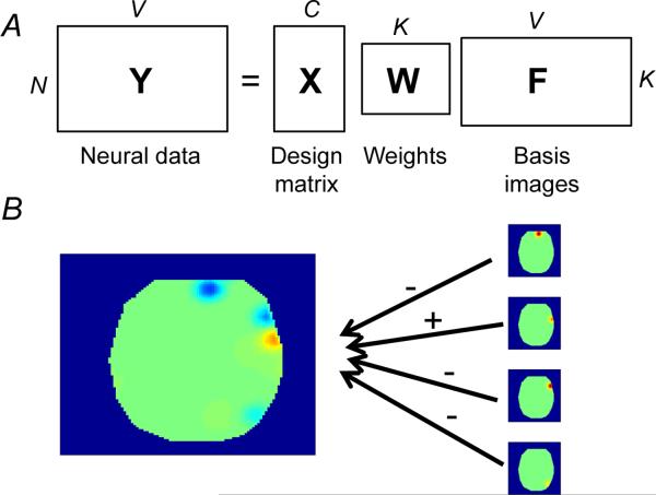
We first present the model for a single subject, shown schematically in Figure 1. In the next section we elaborate this model hierarchically to multiple subjects. Let C be the number of covariates, N be the number of observations, K be the number of latent sources, and V be the number of voxels. The model consists of the following variables (see Figure 1A for a representation in terms of matrix factorization):
X : N × C design matrix containing each covariate's timeseries. Covariates can be continuous or discrete. We shall sometimes refer to discrete covariates as “classes.” Note that the design matrix can accomodate all the standard embellishments used in GLM analyses, such as haemodynamic convolution, temporal filtering, and nuisance regressors (Friston et al., 1994).
W : C × K real-valued weight matrix encoding how each covariate loads on each source. The weights play the same role as coefficients in traditional voxel-based GLM analyses, expressing how much each source (rather than each voxel) is activated in response to changes in each covariate.
F : K × V non-negative real-valued basis image matrix encoding the canonical spatial pattern (over voxels) associated with each latent source. Each basis image fk is a deterministic function of a set of parameters ωk (location and width of each source; see next section).
Y : N × V real-valued fMRI data matrix, the pattern of activity at each observation.
R : V × D real-valued location matrix, specifying, in D-dimensional coordinates (usually D = 3), the location of each voxel. In order to specify a uniform spatial prior on the source locations (see next section), we normalize the image dimensions to the [0, 1] interval, so that rv ε [0, 1]D.
Figure 1. Generative model.
(A) Matrix factorization view of TLSA. (B) A schematic illustrating how basis images (right) combine to form the class-conditional activation map for a single class (left). Plus and minus symbols indicate positive and negative weights, respectively.
2.2. Generative model
We assume the observed fMRI data arise from a covariate-dependent superposition of latent sources (Figure 1B):
| (1) |
where . This model can be written in matrix notation:
| (2) |
We construct the basis image fk associated with latent source k using a spatial basis function with parameters ωk. While a variety of basis functions are acceptable, for our applications we use a spherical radial basis function with parameters ωk = {μk, λk}, where μk ε [0, 1]D is a source location and is a spatial width:
| (3) |
The source location μk specifies the region of the brain in which source k concentrates its energy, and the width specifies its spatial extent.
We place the following prior distributions on the parameters:
| (4) |
| (5) |
| (6) |
While these are the priors that we use in the study, we note that TLSA can accommodate other priors (i.e., the inference algorithm we present in the next section does not require conjugate priors). In section 3.1, we using synthetic data to assess the sensitivity to choice of prior.
We now describe the hierarchical extension of this model. The basic idea behind hierarchical models is that parameters are coupled together by virtue of being drawn from a common distribution; this allows sharing of structure between different parameters while still allowing between-parameter variability (see Gelman and Hill, 2007, for a general introduction to hierarchical modeling). In hierarchical TLSA, each subject's parameters θs = {Ws, ωs} are assumed to arise from Gaussian perturbations of the group-level parameters θs = {Ws, ωs},
| (7) |
| (8) |
| (9) |
We truncate the Gaussians for μ ε [0, 1] and λ ε (0, ∞) to ensure these variables stay within the appropriate range. We give the group-level parameters θ0 the same priors as described above for the non-hierarchical version (Eqs. 4–6). The hierarchical model makes the assumption that sources are shared across subjects, but their location, width and loading vector can vary from a group-level template. In this way, statistical structure is shared across subjects while allowing for individual differences. In the remainder of the paper, we will refer to the hierarchical and non-hierarchical versions of TLSA as “TLSA-H” and “TLSA-NH,” respectively.
2.3. Inference
Our goal is to compute the posterior over the hidden variables θ = {W0:S; ω0:S} given the observed variables X and Y:
| (10) |
As for many complex Bayesian models, the normalizing constant (marginal likelihood) is intractable to compute. We therefore approximate the posterior with a set of L samples generated by Markov Chain Monte Carlo (MCMC; Robert and Casella, 2004). In particular, we apply the Metropolis algorithm (Metropolis and Ulam, 1949) to obtain samples from the posterior. Letting θ(l) denote the current state of the Markov chain, the Metropolis algorithm iteratively proposes a new value θ′ ~ q(θ(l)) and accepts this proposal with probability
| (11) |
where q(θ; θ(l)) = q(θ(l); θ). If the proposal is rejected, then θ(l) = θ(l−1). After a burn-in period, this Markov chain will reach its stationary distribution, which is the posterior (Eq. 10). Using these samples, the posterior is approximated by:
| (12) |
where δ[·, ·] is 1 if its arguments are equal and 0 otherwise.
The MCMC algorithm converges when the Markov chain reaches its stationary distribution. One pitfall of MCMC methods is the existence of local modes in the posterior, which can cause the chain to converge slowly. As is common with MCMC methods (Robert and Casella, 2004), we attempted to improve convergence time by dividing θ into a set of coordinates, each with its own proposal distribution, and update these iteratively. We used Gaussian proposal distributions for and , and Gamma distributions for ; in all cases, the distributions were centered on the current sample. We tuned the parameters of these proposal distributions to achieve acceptance rates greater than 15 percent, although we did comprehensively explore the parameter space. Specifically, we used a proposal variance of 0.2 for the weight updates, 0.1 for the source center updates, and 0.1 for the source width updates. For good initialization of the source centers, we used the mean activation maps for all conditions to find task-relevant locations, and seeded the source centers by randomly drawing from these locations. For a 32 × 32 image with 100 datapoints, TLSA-NH takes 84 seconds to perform 1000 iterations on a 64-bit, 2.53Ghz dual-core processor.
2.4. A hypothesis-testing framework
Once TLSA has been fit to data, we want to test specific hypotheses about the parameter estimates. For example, we may want to test the hypothesis that the loading of source k on class c is greater than 0. The approximate posterior produced by MCMC allows us to easily calculate this probability by counting the proportion of samples for which wck > 0. More generally, let denote a hypothesis and be a binary indicator that is equal to 1 if is true given ק and 0 otherwise. The posterior probability that is true is:
| (13) |
The resulting “posterior p-value” quantifies the degree of belief in after observing the data (see Friston et al., 2002, for a comparison between classical and Bayesian hypothesis-testing). With TLSA, the hypotheses are typically about latent sources rather than voxels. This allows the researcher to investigate and reason about spatially extended activations directly, without requiring post-hoc procedures such as cluster-thresholding and correction for multiple comparisons (Friston et al., 1996).
One hypothesis class that is relevant from the perspective of traditional fMRI analysis is the linear contrast, ηwk, where η is a 1 × C vector of contrast coefficients and w is the kth column of W (which could be either subject- or group-level weights). Usually the contrast vector isolates the difference between two experimental conditions (i.e., two classes in the multi-class setting), and the hypothesis is whether the new random defined by the contrast is greater (or less than) γ (e.g., Friston et al., 1994). To construct model-based thresholded contrast maps, we first calculate P(wik − wjk > γ) for each source separately, where γ is an activation threshold, and i and j represent the two classes we are interested in contrasting. We then remove those sources for which the probability is below some con dence threshold; following Friston and Penny (2003), we recommend a probability threshold of 0.95, which we use in the experiments reported below (with γ = 0). Finally, we calculate the model-based contrast map by subtracting the class-conditional maps using only the sources that have survived thresholding.
Because some sources will inevitably be used to capture noise in the data, an important task is to identify which sources carry “signal” and which sources carry “noise.” The Bayesian hypothesis testing machinery can be used for this purpose: Weights for noise sources will tend to have low probability of deviating from zero.
Note that Bayesian hypothesis tests are fundamentally different from classical (frequentist) hypothesis tests based on p-values (Wagenmakers and Grüunwald, 2006). The posterior probability of a hypothesis represents the researcher's subjective degree of belief in the hypothesis; this degree of belief is not necessarily well-calibrated with the true probability, and depends on the specification of priors. As such, researchers should not treat the posterior probability threshold according to the same standards as p-values: a 0.95 posterior probability threshold is not related meaningfully to a 0.05 p-value threshold.
2.5. Comparison against other models
As a baseline against which to compare TLSA, we will study Gaussian Naive Bayes (GNB) and multi-nomial logistic regression (LR) models on data pre-processed by singular value decomposition (SVD) or independent components analysis (ICA) with varying numbers of components. These models have been shown to achieve good performance when applied to several previous fMRI datasets (McKeown and Sejnowski, 1998; Svensén et al., 2002; Mitchell et al., 2004; Hu et al., 2005; Chen et al., 2006). Details of these models are provided in the Appendix. We use the notation “SVD-GNB” to denote GNB operating on latent components derived from SVD (and likewise for other combinations, e.g., SVD-LR, ICA-GNB, etc.).
We emphasize that only our method, and not the alternatives to which we compare, can make inferences about latent sources. The other methods are fundamentally voxel-based. Thus, for researchers interested in making inferences about the latent spatial structure of their data, our method offers a unique advantage. The purpose of the quantitative comparisons is to show that our method performs comparably on other tasks to which the alternative model are commonly applied.
2.6. Evaluation metrics
We evaluate the models described above according to four different metrics. Each of these metrics is applied to held-out data using a cross-validation procedure, where one run (from each subject) is left out of the training set and used as an independent test set.
Predictive probability: Given a test set of activity patterns Y′, how well can the model predict X′? We measure predictive performance by calculating the posterior predictive probability of the test covariates under the model. In other words, we calculate how likely the true covariates are under the model, using the maximum a posteriori (MAP) parameter estimates. This metric is more sensitive than accuracy, since it does not apply a hard threshold to the model's predictions.
Reconstruction error: Given a test set of covariates X′, what is the mean-squared reconstruction error (MSE) for predicting Y′?
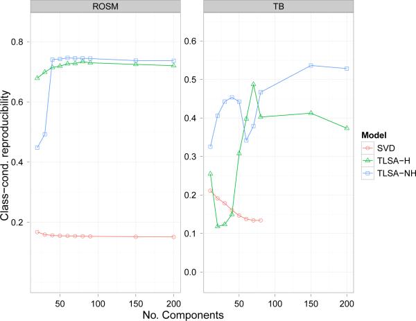
Class-conditional reproducibility: How similar are the inferred class-conditional densities across different subsets of the data? We measured this by calculating the average similarity between the class-conditional mean images (backprojecting the SVD-based parameter estimates into the original voxel space) for pairs of cross-validation folds, where similarity is measured by the correlation between the image vectors. This metric measures how well a model captures the global pattern evoked by a class.
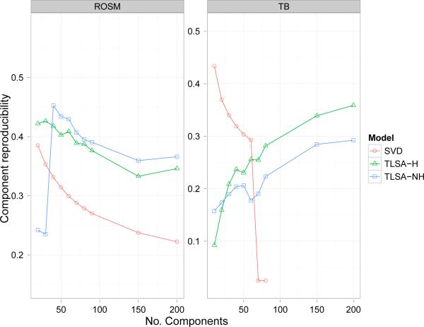
Component reproducibility: How similar are the inferred basis images (components) across different subsets of the data? We measured this by greedily matching components across cross-validation folds (using a Pearson correlation metric) and then calculating component-wise correlation for pairs of cross-validation folds.
3. Results
In this section, we present analyses of synthetic and real fMRI data.
3.1. Analyses of synthetic data
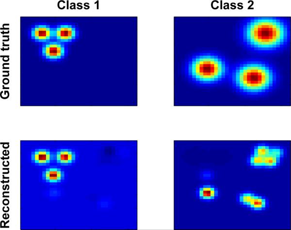
We first evaluated TLSA on synthetic data, consisting of 6 sources and 2 classes (blocked design, although this property is immaterial, since all the models we consider assume exchangeable datapoints). The synthetic dataset (N = 40) was defined on a 32 × 32 pixel image and corrupted by zero-mean Gaussian noise with σy = 0.1. The ground-truth class-conditional maps are shown in Figure 2. These maps represent the expected activation pattern for each class:
| (14) |
where each source surface was drawn from a zero-mean Gaussian process with Matérn covariance function (see Rasmussen and Williams, 2006). While generally smooth, these surfaces do not assume a radial basis function shape, and can generally be quite complex. Fitting TLSA to these data will help understand the model's performance the underlying generative process is misspecified. We fit TLSA-NH to the data with K = 40, κ = 100, τ = 1, σ = 0.1, running the MCMC algorithm for 5000 iterations. The tted model appears to capture the structure of the class-conditional maps (Figure 2), with the extra sources allowing the model to compensate for the misspecification of the prior.
Figure 2. Class-conditional maps for synthetic data.
(Top) Simulated class-conditional maps for two classes. (Bottom) TLSA-NH reconstructions of the class-conditional maps (see text for details).
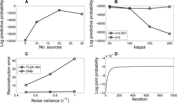
Next, we examined how the results changed with number of sources (K). Splitting the dataset into a training and test set, we found that held-out predictive probability increases with K for the synthetic dataset, peaking at K = 20 and declining thereafter (Figure 3A). This suggests that overestimating the number of source in the data may be useful for overcoming model misspecification, but using too many sources can result in over-fitting. Thus, there is an “optimal” number of sources that will vary from dataset to dataset.
Figure 3. Synthetic data results.
(A) Held-out predictive probability of TLSA-NH increases with K for the synthetic dataset; (B) held-out predictive probability of TLSA-NH as a function of hyperparameter settings; (C) held-out reconstruction error of TLSA-NH and GNB as a function of noise level; (D) Trace of the joint data and latent variable log probability for a single MCMC run.
In order to assess the sensitivity of these results to hyperparameter settings, we varied the weight prior variance σ2 and source width parameter κ, re-estimating the held-out predictive probability for each setting. We show the resulting performance curves in Figure 3B. Our results demonstrate that the held-out predictive probability is relatively constant over a wide range of different settings of κ when σy is small, but declines as a function of κ when σ is large. It is thus generally better to use large sources (small κ), since this appears to be more robust to changes in the weight prior.
We next investigated how the model performs as the noisiness of the data increases. We found that reconstruction performance maintains superiority over GNB across a range of noise levels (Figure 3C). One explanation for this finding is that GNB is estimating many more parameters than TLSA, and as a consequence can more easily fit noise, leading to poor generalization performance.
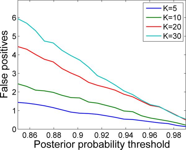
A related question is what TLSA does when there is only noise. More specifically, how often will TLSA erroneously infer a significant effect when none exists? To answer this question, we repeatedly fit TLSA-NH with a varying numbers of sources to data consisting entirely of zero-mean, unit variance Gaussian noise. For each repetition and each sample we then calculated the linear contrast between the weights of the two classes. A contrast for a source was deemed significant if the proportion of sample-contrasts greater or less than 0 exceeded a variable posterior probability threshold. As shown in Figure 5, the number of false positives becomes vanishingly small as the probability threshold increases. Furthermore, the difference in the number of false positives between models with different values of K also vanishes with an increasing probability threshold. Thus, TLSA appears to sensitively control the number of false positives in a manner that is relatively independent of K for sufficiently large probability thresholds.
Figure 5. False positives under noise conditions.
Each curve corresponds to a model with a different number of sources (K). A false positive occurs when a weight contrast is deemed significant for a source at a particular probability threshold, with γ = 0. See text for details.
Another question regarding the training of our model is convergence of the MCMC sampler. While assessing convergence to the stationary distribution (i.e., the posterior) is notoriously difficult, we can evaluate the more modest goal of convergence to a local mode. Figure 3D shows the trace of the joint log-likelihood as a function of iteration for a single MCMC run. The trace plot demonstrates convergence to a local mode after approximately 200 iterations.
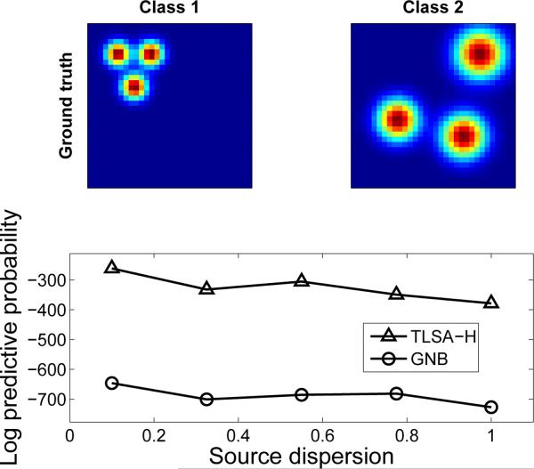
Finally, we investigated how the performance of the hierarchical model changes as a function of source dispersion ζ. This parameter dictates how similar spatial activations are across subjects. In order to systematically manipulate source dispersion, we used radially-shaped sources, as shown in Figure 4A. We found that performance of TLSA-H degrades as ζ increases, but is still better than GNB (Figure 4B). To get a sense of what these values of ζ mean, for ζ = 0.5 roughly half the sources centers will be displaced by more than one voxel. Taken together, these results indicate that the model is robust to a variety of violations of the generative assumptions.
Figure 4. Effects of source dispersion.
(A) Synthetic group-level class-conditional maps used in the simulation. (B) Held-out predictive probability of TLSA-H and GNB as a function of source dispersion.
3.2. Real datasets
We next fit the models described above to two fMRI datasets. The first, collected by McDuff et al. (2009), involved subjects studying lists of nouns. We will refer to this dataset as “ROSM” (retrieval orientation and source memory). On each trial, subjects were presented with a noun and asked to perform one of 3 encoding tasks (“artist,” “function” or “read”; see McDuff et al., 2009, for details). We treat each of these encoding tasks as a separate class; thus, xnc = 1 if the subject was performing task c at time n. Data were not coregistered prior to analysis. Each subject's data (324 trials per subject, divided into 6 runs) were sub-sampled in all 3 image planes (to ease the computational expense of model-fitting), yielding 5000–6000 voxels for each subject. The data were then z-scored within each run.
The second dataset (“TB,” or tools/buildings), collected by Mason and Just (unpublished), involved subjects viewing words for 3 seconds, followed by a blank screen for 3 seconds. Each word was either the name of a type of tool or of a type of building (i.e., there were 2 classes), and the subject's task was to think about the word and its properties while it was displayed, and to not think about anything during the blank screen. There were 7 different exemplars of each of the two categories and 6 blocks. All 14 exemplars were shown without repetition in each block, for a total of 84 trials per subject. An fMRI volume was collected every second, using 3 × 3 × 5mm voxels in a 64 × 64 × 16 grid. Voxels outside of cortex were filtered out using an anatomical mask, yielding 15000–20000 voxels for each subject. The images 4, 5, 6 and 7 seconds after stimulus onset in each trial were averaged together into a single example, which was then z-scored across voxels (within runs). Data were not coregistered prior to analysis. For the SVD-based analyses, we truncated K at 60, since the singular values for larger K will be close to 0 (due to the small number of trials).
For both datasets, we ran the MCMC sampler for 5000 iterations with different values of K (the number of latent sources), using the highest-scoring sample (the maximum a posteriori estimate) for visualization and prediction purposes. We found that parameter estimates stabilized after about 2000 iterations. We used the following hyperparameter settings: τ = 1, σ = 0.1, σ0 = 1, ζ = 0.1, ρ = 1, κ = 400, ν = 10.
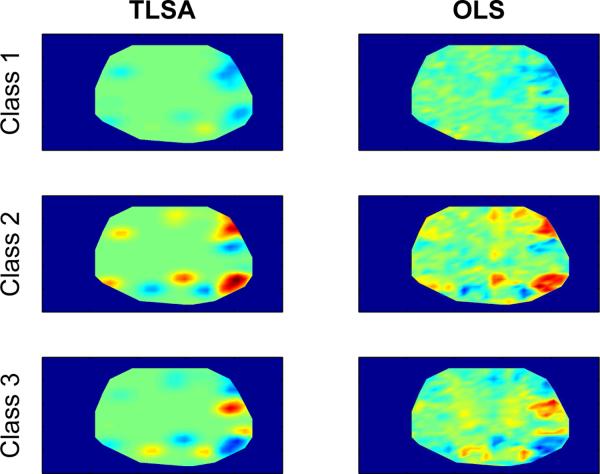
Figure 6 (left) shows example class-conditional maps for a single subject in the ROSM dataset with K = 80. For comparison, the right column of Figure 6 shows the map of ordinary least-squares estimates, which in this case are equivalent to the class-conditional means for each voxel.
Figure 6. Example class-conditional maps for the ROSM dataset.
Each row represents a different class. The left column shows the predicted class-conditional maps under the fitted model; the right column shows the voxel-wise ordinary least-squares (OLS) estimates for each class, which is equivalent to the class-conditional means.
3.3. Prediction, reconstruction and reproducibility
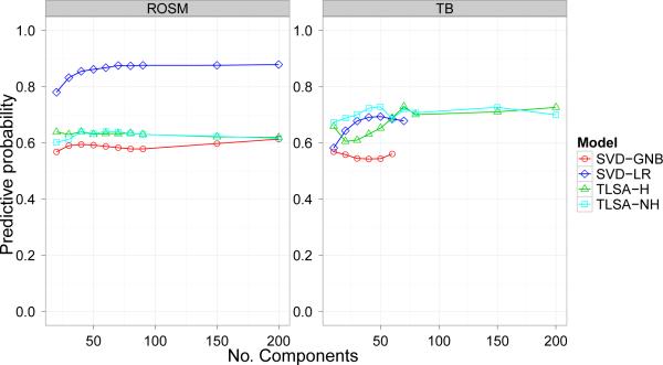
Predictive performance of the models is shown in Figure 7. We found that the ICA preprocessing produced inferior performance compared to SVD preprocessing across all our metrics (and for all tested values of K); we therefore exclude this model from our figures and discussion. All 4 remaining models perform better than chance (1/3 for the ROSM dataset, 1/2 for the TB dataset). Generally speaking, the SVD-GNB model performed most poorly, and, for K > 60, the two versions of TLSA performed comparably to one another. SVD-LR performed much better than the other models on the ROSM dataset, but was inferior to TLSA on the TB dataset for K > 60.
Figure 7. Prediction results.
Average predictive probability for held-out data as a function of number of components (latent sources or SVD basis images). Note that GNB and LR are cut off at 60 for the TB dataset because the number of SVD with non-zero singular values cannot exceed the number of datapoints in the training set.
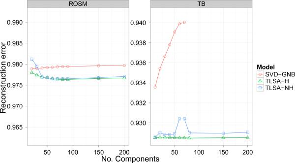
Reconstruction performance is shown in Figure 8. Note that this metric, since it operates only over the latent components, is identical for SVD-LR and SVD-GNB (we therefore denote these models together as “SVD”). Over a wide range of K values, the reconstruction performance of TLSA is superior to that of SVD. However, the hierarchical and non-hierarchical versions of TLSA are indistinguishable in terms of reconstruction performance.
Figure 8. Reconstruction results.
Average mean-squared reconstruction error for held-out data as a function of number of components (latent sources or SVD basis images). Note that on this plot lower values indicate better performance.
Reproducibility performance is shown in Figures 9 and 10. Note that component-reproducibility (like the reconstruction metric) depends only on the latent components, and hence is identical for SVD-LR and SVD-GNB. For the ROSM dataset, both variants of TLSA outperformed SVD for both reproducibility metrics, although there was no clear pattern of superiority for a single variant. For the TB datset, the results were mixed. For class-conditional reproducibility, TLSA outperformed SVD-GNB, but for component reproducibility the opposite pattern was obtained. There was a trend for SVD's component reproducibility to decrease with increasing K, while TLSA's performance tended to increase with K. There also is a dip in the performance of TLSA-NH for intermediate values of K on the TB dataset. This appears to be a reliable effect, in that we found it using multiple chains with different initializations; we do not have an explanation for this effect.
Figure 9. Class-conditional reproducibility results.
Y-axis represents the class-conditional reproducibility score.
Figure 10. Component reproducibility results.
Y-axis represents the component reproducibility score.
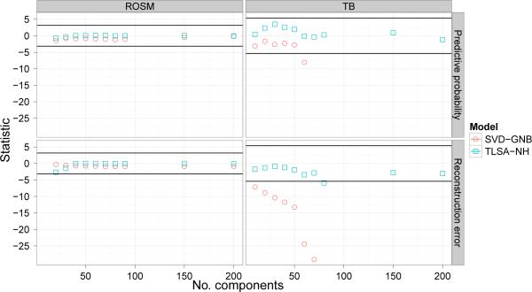
To statistically assess the difference in performance between the models, We computed paired-sample t-tests between models for each setting of K. We concentrate on comparing TLSA with SVD-GNB, since it is not possible to calculate class-conditional reproducibility or reconstruction metrics for LR.1 Figure 11 shows the t-statistics for comparisons of SVD-GNB and TLSA-NH with TLSA on our prediction and reconstruction metrics; horizontal lines denote the 0:05 p-value threshold for signi cance. This threshold was Bonferroni-corrected to take into account our multiple-testing procedure (20 tests per metric for ROSM, 16 for TB). Thus, 0 represents indistinguishable performance compared to TLSA, and positive t-values indicate superior performance of the model relative to TLSA.
Figure 11. Prediction and reconstruction test statistic results.
Y-axis represents the t-statistic for paired-sample comparison of predictive probability (top row) and reconstruction error (bottom row) against TLSA. Horizontal lines denote Bonferroni-corrected 0.05 p-value threshold.
Figure 11 indicates that most of these comparisons are non-significance, except for reconstruction error on the TB dataset, for which SVD performs much worse than TLSA. Thus, the pattern of prediction and reconstruction results suggests that both variants of TLSA are competitive with, if not superior to, SVD-GNB.
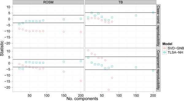
Figure 12 shows analogous t-statistics for the reproducibility metrics. For the ROSM dataset, TLSA is generally superior to SVD on both metrics. For the TB dataset, SVD is superior to TLSA for small K but not for large K on component reproducibility; there does not appear to be a significance advantage for either model on class-conditional reproducibility. As with the other metrics, TLSA does not display a decisive advantage over TLSA-NH.
Figure 12. Reproducibility test-statistic results.
Y-axis represents the t-statistic for paired-sample comparison against TLSA. Horizontal lines denote Bonferroni-corrected 0.05 p-value threshold.
3.4. Hypothesis-testing
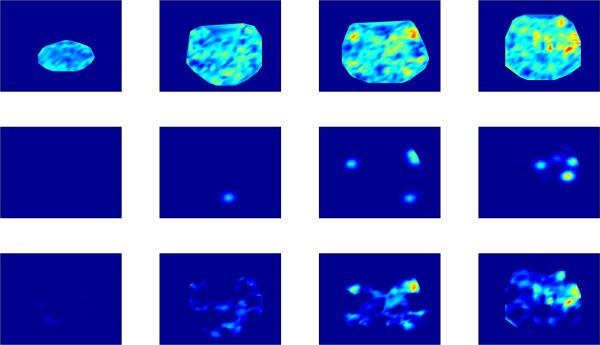
To illustrate the Bayesian hypothesis testing framework, we examined the contrast between two classes (class 1 - class 2) for a single subject in the ROSM dataset. The empirical contrast (difference between class means) is shown for different slices in the top row of Figure 13. The model-based contrast maps are shown in the middle row, calculated according to the procedure described in Section 2.4. The bottom row of Figure 13 shows the contrast resulting from spatially-regularized voxel-wise parameter estimates (Penny et al., 2005). Spatial regularization is induced by a Gaussian Markov random field prior on the parameters. The maps were thresholded according to a 0:95 posterior probability threshold, such that they are comparable to the thresholded TLSA contrast maps. These results illustrate that the posterior probability maps produced by TLSA are comparable to what one would obtained using a spatially-regularized GLM analysis, and can be interpreted in a similar way. We emphasize that inferential statistics based on these maps represent inferences about spatially-extended latent sources rather than voxels, which means that additional operations (e.g., cluster-size thresholding) are unnecessary.
Figure 13. Example hypothesis test.
(Top) Empirical contrast (difference between class means) for class 2 versus class 1. Each column represents a slice of the contrast map. (Midle) TLSA contrast map thresholded at posterior probability greater than 0.95. (Bottom) Spatially-regularized GLM-based contrast map, thresholded at 0.95 posterior probability.
4. Discussion
In this paper, we presented TLSA, a new model of fMRI spatial statistics in which neural activity arises from covariate-dependent superposition of latent sources. We evaluated this model using several metrics and compared it to Naive Bayes and logistic regression models, demonstrating that TLSA can achieve good levels of performance. We also presented a Bayesian hypothesis-testing framework that allows researchers to test a wide variety of hypotheses (e.g., linear contrasts) about the latent sources inferred from the data. The advantage of working with latent sources rather than voxel-specific parameters is that the latent sources have intrinsic spatial extent and are thus suitable for capturing spatial patterns without the need for post-hoc corrections like cluster-size thresholds.
TLSA addresses several problems in fMRI analysis, including spatial alignment and smoothing, as well as providing a method for multivariate analysis. We showed that TLSA is competitive with widely-used generative (GNB) and discriminative (LR) models according to several different performance metrics. For prediction and reconstruction tasks TLSA displays either equivalent or better performance compared to GNB, and TLSA outperforms GNB in reproducibility over a range of values of K. These results provide evidence for the usefulness of the latent sources discovered by TLSA; the hypothesis-testing framework allows us to move beyond simple prediction and reconstruction to answering scientific questions about the latent sources.
When we trained the models on more data (Figures 7–12), we did not observe any reliable differences between the performance of TLSA and TLSA-NH according to most of our performance metrics. One possible explanation for this finding is that there was insufficient spatial homogeneity across subjects in the datasets we analyzed to provide the hierarchical model with an advantage over its non-hierarchical counterpart. Another possibility is that the sampler was stuck in local modes, corresponding to the non-hierarchical solution.
4.1. Related work
In addition to the SR-GLM and MVPA approaches mentioned in the Introduction, there exist a number of other approaches to spatial modeling of brain activations. Kiebel et al. (2000) constructed anatomically informed basis functions by segmenting the gray matter into a vertex-based surface with a Gaussian spatial interpolant (essentially identical to the spatial basis functions we used). They then optimized a set of regression coefficients for these basis functions. The mathematical form of their model is similar to ours, but we infer the parameters of the basis functions from functional data, whereas they infer them from anatomical data. This allows us to infer fewer numbers of basis functions, since the number of functionally relevant areas of the brain tend to be much fewer than number of vertices required to accurately model the anatomical surface (Kiebel et al. report 130,000 as a typical number). An interesting problem for future work is how to incorporate anatomical information into TLSA.
A different approach was taken by Lindeberg et al. (1999), who used the concept of a “scale-space primal sketch” from computer vision (Lindeberg, 1994). A signal's scale-space representation is the original signal convolved with a Gaussian kernel over a spectrum of variances. Thus, coarser spatial scales are de ned by convolutions with higher-variance Gaussians. The scale-space primal sketch represents a spatially-varying signal (e.g., a brain volume) as a multi-scale tree whose leaves are blobs (extended local extrema). Lindeberg et al. (1999) present an algorithm for extracting these blobs from brain activation data. Remarkably, this algorithm has almost no free parameters. The authors do not provide a statistical framework for assessing the significance of blobs. TLSA does not address multi-scale spatial structure. It is an avenue for future research.
Another line of work has focused on modeling the map of summary statistics produced by mass-univariate GLM analyses (Xu et al., 2009; Kim et al., 2010). To account for spatial structure in these maps, each summary statistic is assumed to arise from a mixture of Gaussians, where the mean of each mixture component represent the spatial location of a “blob” (akin to latent sources in TLSA). The mixture formulation allows the marginal distribution of spatial activations to be non-Gaussian. The work of Kim et al. (2010) places a nonparametric prior over the mixture components, allowing the number of components to be learned from the data, whereas Xu et al. (2009) use reversible-jump MCMC to infer the model dimensionality. Although this work is not directly comparable to ours (since we are modeling the entire fMRI timeseries, whereas they are modeling summary statistics), the idea of using latent spatial components is in the same spirit. One technical difference is that our model is inherently a factor model, in that we allow multiple sources to contribute to each voxel, whereas the work of Xu et al. (2009) and Kim et al. (2010) attempt to infer a single component for each voxel. One reason to think that a factor model is more appropriate is the observation that a single brain region may be part of several functional networks (e.g., LaBar et al., 1999).
4.2. Future directions
There are a number of limitations of TLSA and our inference algorithm. First, it may be desirable to relax some of the assumptions of the generative model. In particular, we assume that all within-class heterogeneity (in the discrete covariate case) is due to random observation noise, an assumption that is unlikely to be true. For example, there may be systematic changes in brain activity that are due to unmodeled causes, such as attention. The SVD-based methods are able to at least partly model this source of variance. One possibility is to change the observation noise model to be a Student t-distribution, which would arise in the case where the weights were allowed to vary across observations according to a Gaussian distribution. Alternatively, we could model observation-specific weights with a mixture of Gaussians. Another limitation of the generative model is that it assumes the number of latent sources (K) to be known. This problem can be addressed using cross-validation to select K. Alternatively, we could address the problem nonparametrically by placing a hierarchical Dirichlet process prior over the latent sources (Teh et al., 2006), which would discover the number of sources automatically, while allowing sharing of sources across subjects.
On the algorithmic front, our MCMC sampler suffers from long computation times. Although more efficient sampling algorithms are possible (e.g., Hybrid Monte Carlo; Duane et al., 1987), we have found that these do not substantially improve speed or convergence for these datasets. An alternative is to use variational methods (Jordan et al., 1999), which convert the inference problem into an optimization problem by searching for the approximate posterior within some constrained family of densities that best approximates the true posterior. Variational methods have been shown to achieve excellent performance with much less computational overhead compared to MCMC methods (Bishop, 2006).
Although there are many avenues for future improvement, the model developed in this paper shows promise as a useful addition to the analytical toolbox for fMRI data. The flexibility of the probabilistic modeling framework will allow us to easily extend and refine these preliminary explorations, as well as integrate neuroimaging data with other information, such as behavior and computational models of cognition.
Acknowledgements
We thank Per Sederberg, Matt Hoffmann, Richard Socher, Katherine Heller, Martin Lindquist and Michael Todd for helpful discussions. We are also grateful to Rob Mason and Marcel Just of the Center for Cognitive Brain Imaging at Carnegie-Mellon University for sharing the TB dataset. This research was supported by the NSF/NIH Collaborative Research in Computational Neuroscience Program, grant number NSF IIS-1009542. David M. Blei is supported by ONR 175-6343, NSF CAREER 0745520, AFOSR 09NL202, the Alfred P. Sloan foundation, and a grant from Google. SJG was supported by a Quantitative Computational Neuroscience training grant from the National Institute of Mental Health as well as a National Science Foundation Graduate Research Fellowship.
Appendix: alternative models
4.3. Singular value decomposition
SVD decomposes the neural data into a set of 3 matrices:
| (15) |
where U is an N × N orthonormal “output” basis set (the eigenvectors of YYT), Q is a V × V orthonormal “input” basis set (the eigenvectors of YTY), and Σ is an N × V diagonal matrix of singular values, conventionally arranged in descending order. By only retaining the K components with the largest singular values, the neural data can be approximated by the product of lower-rank matrices. We define the low-dimensional SVD approximation of Y as the projection of Y onto the subspace defined by the first K columns of Q (denoted by ):
| (16) |
4.4. Independent components analysis
ICA decomposes the neural data into the product of a source matrix S and a mixing matrix A:
| (17) |
where the source and mixing matrices are chosen to maximize the objective function
| (18) |
Maximizing this objective function is equivalent to maximizing the entropy of the predicted neural signals—the so-called “infomax” principle (Bell and Sejnowski, 1995; Cardoso, 2002). We use the FastICA algorithm of Hyvarinen (2002) to maximize this objective.
4.5. Gaussian naive Bayes
GNB models the joint distribution of the (reduced) neural data and covariates as a product of Gaussians:
| (19) |
We set μ and σ to their maximum likelihood estimates (i.e., the class-conditional empirical means and variances, respectively). It is assumed here that the covariates are multi-class with a uniform prior probability over classes. The version of GNB described here can only be applied to multi-class covariate data, whereas TLSA is designed to work with both continuous and discrete covariate data. See Frank et al. (2000) for extensions of GNB to handle continuous covariate data.
4.6. Logistic regression
LR models the conditional distribution of the covariates given the reduced neural data using a GLM with a softmax link function:
| (20) |
where ηc is a 1 × K vector of regression coefficients. In the case of continuous covariates, the softmax link function is replaced by a linear link function (i.e., linear regression). The regression coefficients can be estimated via maximum likelihood or maximum a posteriori (MAP) estimation. For MAP estimation, a common choice of prior on η (which we adopt here) is a zero-mean Gaussian, which is equivalent to logistic regression with an L2 penalty (Hastie et al., 2001). We chose a penalty parameter of 1, which performed well for our datasets; varying the parameter by an order of magnitude did not have a significant impact on the results.
Footnotes
Publisher's Disclaimer: This is a PDF file of an unedited manuscript that has been accepted for publication. As a service to our customers we are providing this early version of the manuscript. The manuscript will undergo copyediting, typesetting, and review of the resulting proof before it is published in its final citable form. Please note that during the production process errors may be discovered which could affect the content, and all legal disclaimers that apply to the journal pertain.
Component reproducibility will be identical for LR and GNB since it relies only on the SVD components, which are common to both models.
References
- Bell A, Sejnowski T. An information-maximization approach to blind separation and blind deconvolution. Neural Computation. 1995;7(6):1129–1159. doi: 10.1162/neco.1995.7.6.1129. [DOI] [PubMed] [Google Scholar]
- Bishop C. Pattern Recognition and Machine Learning. Springer; 2006. [Google Scholar]
- Bowman F, Caffo B, Bassett S, Kilts C. A Bayesian hierarchical framework for spatial modeling of fMRI data. NeuroImage. 2008;39(1):146–156. doi: 10.1016/j.neuroimage.2007.08.012. [DOI] [PMC free article] [PubMed] [Google Scholar]
- Cardoso J. Infomax and maximum likelihood for blind source separation. Signal Processing Letters, IEEE. 2002;4(4):112–114. [Google Scholar]
- Chen X, Pereira F, Lee W, Strother S, Mitchell T. Exploring predictive and reproducible modeling with the single-subject FIAC dataset. Human Brain Mapping. 2006;27(5) doi: 10.1002/hbm.20243. [DOI] [PMC free article] [PubMed] [Google Scholar]
- Duane A, et al. Hybrid monte carlo. Physics letters B. 1987;195(2):216–222. [Google Scholar]
- Flandin G, Penny W. Bayesian fMRI data analysis with sparse spatial basis function priors. NeuroImage. 2007;34(3):1108–1125. doi: 10.1016/j.neuroimage.2006.10.005. [DOI] [PubMed] [Google Scholar]
- Frank E, Trigg L, Holmes G, Witten I. Naive Bayes for regression. Machine Learning. 2000;41(1):5–15. [Google Scholar]
- Friston K, Holmes A, Poline J, Price C, Frith C. Detecting activations in PET and fMRI: levels of inference and power. NeuroImage. 1996;4(3):223–235. doi: 10.1006/nimg.1996.0074. [DOI] [PubMed] [Google Scholar]
- Friston K, Holmes A, Worsley K, Poline J, Frith C, Frackowiak R, et al. Statistical parametric maps in functional imaging: a general linear approach. Human Brain Mapping. 1994;2(4):189–210. [Google Scholar]
- Friston K, Penny W. Posterior probability maps and SPMs. NeuroImage. 2003;19(3):1240–1249. doi: 10.1016/s1053-8119(03)00144-7. [DOI] [PubMed] [Google Scholar]
- Friston K, Penny W, Phillips C, Kiebel S, Hinton G, Ashburner J. Classical and Bayesian inference in neuroimaging: theory. NeuroImage. 2002;16(2):465–483. doi: 10.1006/nimg.2002.1090. [DOI] [PubMed] [Google Scholar]
- Gelman A, Hill J. Data Analysis Using Regression and Multilevel/hierarchical Models. Cambridge University Press; 2007. [Google Scholar]
- Harrison L, Penny W, Ashburner J, Trujillo-Barreto N, Friston K. Diffusion-based spatial priors for imaging. NeuroImage. 2007;38(4):677–695. doi: 10.1016/j.neuroimage.2007.07.032. [DOI] [PMC free article] [PubMed] [Google Scholar]
- Hastie T, Tibshirani R, Friedman JH. The Elements of Statistical Learning. Springer-Verlag; New York: 2001. [Google Scholar]
- Haxby J, Gobbini M, Furey M, Ishai A, Schouten J, Pietrini P. Distributed and overlapping representations of faces and objects in ventral temporal cortex. Science. 2001;293(5539):2425–2430. doi: 10.1126/science.1063736. [DOI] [PubMed] [Google Scholar]
- Haynes J, Rees G. Decoding mental states from brain activity in humans. Nature Reviews Neuro-science. 2006;7(7):523–534. doi: 10.1038/nrn1931. [DOI] [PubMed] [Google Scholar]
- Hu D, Yan L, Liu Y, Zhou Z, Friston K, Tan C, Wu D. Unified SPM-ICA for fMRI analysis. NeuroImage. 2005;25(3):746–755. doi: 10.1016/j.neuroimage.2004.12.031. [DOI] [PubMed] [Google Scholar]
- Hyvarinen A. Fast and robust xed-point algorithms for independent component analysis. Neural Networks, IEEE Transactions on. 2002;10(3):626–634. doi: 10.1109/72.761722. [DOI] [PubMed] [Google Scholar]
- Jordan M, Ghahramani Z, Jaakkola T, Saul L. An introduction to variational methods for graphical models. Machine Learning. 1999;37(2):183–233. [Google Scholar]
- Kiebel S, Goebel R, Friston K. Anatomically informed basis functions. NeuroImage. 2000;11(6):656–667. doi: 10.1006/nimg.1999.0542. [DOI] [PubMed] [Google Scholar]
- Kim S, Smyth P, Stern H. A Bayesian Mixture Approach to Modeling Spatial Activation Patterns in Multi-site fMRI Data. IEEE transactions on medical imaging. 2010 doi: 10.1109/TMI.2010.2044045. [DOI] [PMC free article] [PubMed] [Google Scholar]
- LaBar K, Gitelman D, Parrish T, Mesulam M. Neuroanatomic overlap of working memory and spatial attention networks: a functional MRI comparison within subjects. NeuroImage. 1999;10(6):695–704. doi: 10.1006/nimg.1999.0503. [DOI] [PubMed] [Google Scholar]
- LaConte S, Anderson J, Muley S, Ashe J, Frutiger S, Rehm K, Hansen L, Yacoub E, Hu X, Rottenberg D. The evaluation of preprocessing choices in single-subject BOLD fMRI using NPAIRS performance metrics. NeuroImage. 2003;18(1):10–27. doi: 10.1006/nimg.2002.1300. [DOI] [PubMed] [Google Scholar]
- Lindeberg T. Scale-space theory: A basic tool for analyzing structures at diffierent scales. Journal of Applied Statistics. 1994;21(1):225–270. [Google Scholar]
- Lindeberg T, Lidberg P, Roland P. Analysis of brain activation patterns using a 3-D scale-space primal sketch. Human Brain Mapping. 1999;7(3):166–194. doi: 10.1002/(SICI)1097-0193(1999)7:3<166::AID-HBM3>3.0.CO;2-I. [DOI] [PMC free article] [PubMed] [Google Scholar]
- McDuff S, Frankel H, Norman K. Multivoxel pattern analysis reveals increased memory targeting and reduced use of retrieved details during single-agenda source monitoring. Journal of Neuroscience. 2009;29(2):508. doi: 10.1523/JNEUROSCI.3587-08.2009. [DOI] [PMC free article] [PubMed] [Google Scholar]
- McKeown M, Sejnowski T. Independent component analysis of fMRI data: examining the assumptions. Human Brain Mapping. 1998;6(5–6):368–372. doi: 10.1002/(SICI)1097-0193(1998)6:5/6<368::AID-HBM7>3.0.CO;2-E. [DOI] [PMC free article] [PubMed] [Google Scholar]
- Metropolis N, Ulam S. The Monte Carlo method. Journal of the American Statistical Association. 1949;44(247):335–341. doi: 10.1080/01621459.1949.10483310. [DOI] [PubMed] [Google Scholar]
- Mitchell T, Hutchinson R, Niculescu R, Pereira F, Wang X, Just M, Newman S. Learning to decode cognitive states from brain images. Machine Learning. 2004;57(1):145–175. [Google Scholar]
- Nichols T, Holmes A. Nonparametric permutation tests for functional neuroimaging: a primer with examples. Human Brain Mapping. 2002;15(1):1–25. doi: 10.1002/hbm.1058. [DOI] [PMC free article] [PubMed] [Google Scholar]
- Norman K, Polyn S, Detre G, Haxby J. Beyond mind-reading: multi-voxel pattern analysis of fMRI data. Trends in Cognitive Sciences. 2006;10(9):424–430. doi: 10.1016/j.tics.2006.07.005. [DOI] [PubMed] [Google Scholar]
- O'Toole A, Jiang F, Abdi H, Péenard N, Dunlop J, Parent M. Theoretical, statistical, and practical perspectives on pattern-based classi cation approaches to the analysis of functional neuroimaging data. Journal of cognitive neuroscience. 2007;19(11):1735–1752. doi: 10.1162/jocn.2007.19.11.1735. [DOI] [PubMed] [Google Scholar]
- Penny W, Trujillo-Barreto N, Friston K. Bayesian fMRI time series analysis with spatial priors. NeuroImage. 2005;24(2):350–362. doi: 10.1016/j.neuroimage.2004.08.034. [DOI] [PubMed] [Google Scholar]
- Rasmussen C, Williams C. Gaussian Processes for Machine Learning. The MIT Press; 2006. [Google Scholar]
- Robert C, Casella G. Monte Carlo Statistical Methods. Springer Verlag; 2004. [Google Scholar]
- Svensén M, Kruggel F, Benali H. ICA of fMRI group study data. NeuroImage. 2002;16(3):551–563. doi: 10.1006/nimg.2002.1122. [DOI] [PubMed] [Google Scholar]
- Teh Y, Jordan M, Beal M, Blei D. Hierarchical dirichlet processes. Journal of the American Statistical Association. 2006;101(476):1566–1581. [Google Scholar]
- Wagenmakers E, Grünwald P. A Bayesian perspective on hypothesis testing. Psychological Science. 2006;17(7):641. doi: 10.1111/j.1467-9280.2006.01757.x. [DOI] [PubMed] [Google Scholar]
- Woolrich M, Jenkinson M, Brady J, Smith S. Fully Bayesian spatio-temporal modeling of fMRI data. IEEE transactions on medical imaging. 2004;23(2):213–231. doi: 10.1109/TMI.2003.823065. [DOI] [PubMed] [Google Scholar]
- Worsley K, Marrett S, Neelin P, Vandal A, Friston K, Evans A, et al. A unified statistical approach for determining significant signals in images of cerebral activation. Human Brain Mapping. 1996;4(1):58–73. doi: 10.1002/(SICI)1097-0193(1996)4:1<58::AID-HBM4>3.0.CO;2-O. [DOI] [PubMed] [Google Scholar]
- Xu L, Johnson T, Nichols T, Nee D. Modeling Inter-Subject Variability in fMRI Activation Location: A Bayesian Hierarchical Spatial Model. Biometrics. 2009;65(4):1041–1051. doi: 10.1111/j.1541-0420.2008.01190.x. [DOI] [PMC free article] [PubMed] [Google Scholar]


